IoU / Jaccard in Machine Learning
Let's start with the most fundamental question in computer vision evaluation: how do you measure if your model's prediction is correct?
For classification, it's straightforward -- the predicted class either matches the ground truth or it doesn't. But for tasks where you need to localize objects in space -- object detection, instance segmentation, semantic segmentation -- you're comparing regions, not discrete labels. A predicted bounding box might overlap 90% with the ground truth, or 50%, or 10%. At what threshold do you declare success?
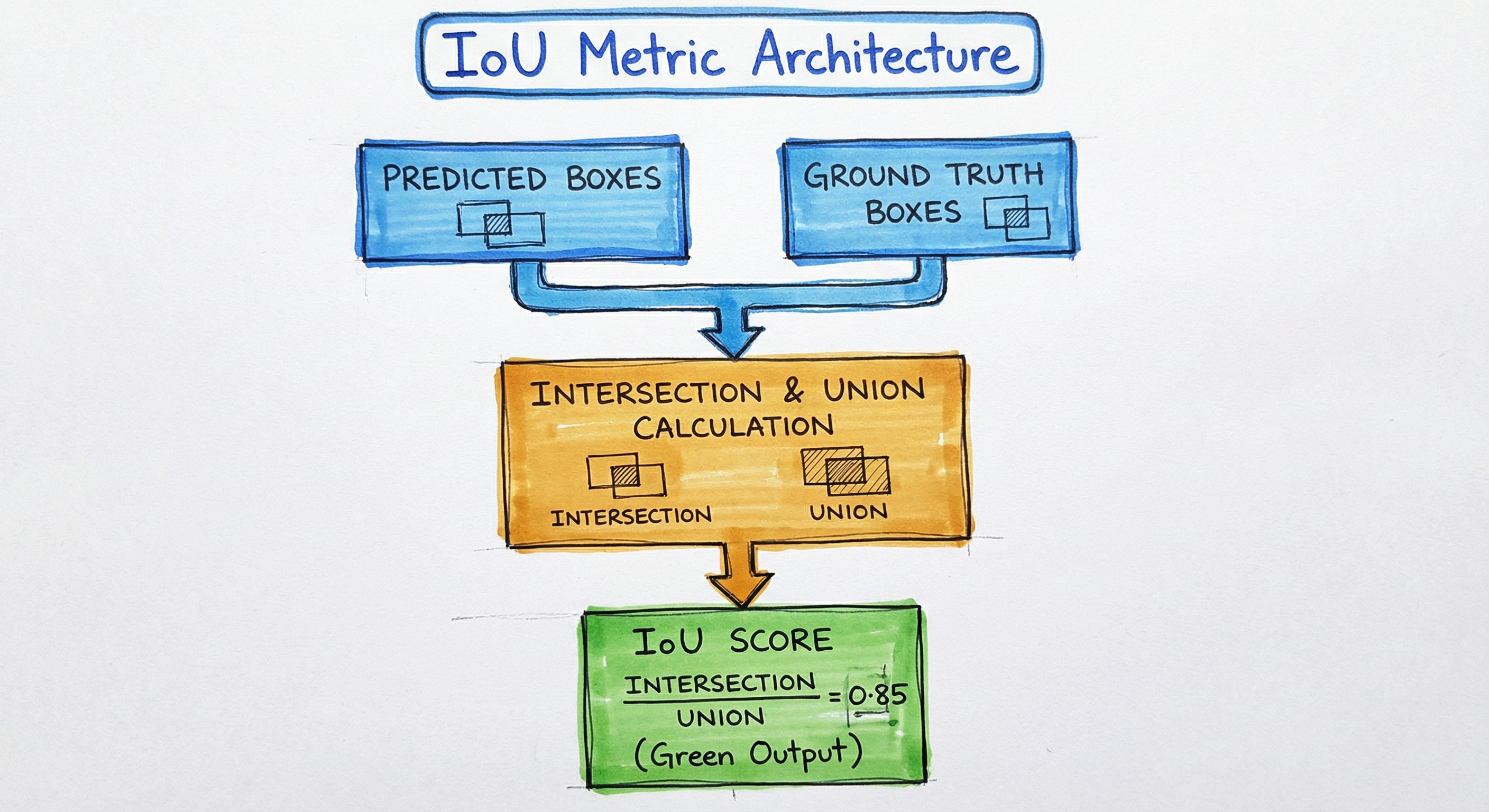
Intersection over Union (IoU), also known as the Jaccard index, provides the answer. It quantifies the spatial overlap between two regions -- typically a predicted bounding box or segmentation mask and its corresponding ground truth -- as a single number between 0 and 1. Zero means no overlap whatsoever. One means perfect alignment.
But here's the crucial insight: IoU isn't just a metric you calculate after training. It's baked into the entire computer vision pipeline. It determines which detections count as true positives when computing mAP. It's used as a loss function during training (IoU loss, GIoU, DIoU, CIoU). It's the primary metric for semantic segmentation (mean IoU). And it's the core of the COCO evaluation protocol that benchmarks state-of-the-art vision models.
Today, from autonomous vehicles navigating Bengaluru's congested streets to medical imaging systems detecting tumors in Indian hospitals, if a system localizes anything in an image, IoU is measuring how well it does that job. Understanding this metric -- and its variants and failure modes -- is non-negotiable for anyone building production computer vision systems.
Concept Snapshot
- What It Is
- A metric that quantifies the spatial overlap between two regions (typically predicted and ground truth bounding boxes or masks) as the ratio of their intersection area to their union area, producing a score from 0 (no overlap) to 1 (perfect match).
- Category
- Evaluation
- Complexity
- Beginner
- Inputs / Outputs
- Inputs: predicted masks/boxes and ground truth masks/boxes (both as coordinate arrays or binary masks). Outputs: IoU score(s) ranging from 0.0 to 1.0, or mean IoU (mIoU) when averaged across classes or instances.
- System Placement
- Used during model evaluation (offline) to compute metrics like mAP and mIoU, and during training (online) as a component of detection/segmentation loss functions.
- Also Known As
- Jaccard index, Jaccard similarity coefficient, IoU score, overlap metric, region overlap
- Typical Users
- Computer vision engineers, ML researchers, Model evaluation engineers, Annotation quality teams, Computer vision product managers
- Prerequisites
- Basic geometry (area calculation), Set theory (intersection, union), Object detection fundamentals, Image segmentation concepts
- Key Terms
- intersectionunionbounding boxsegmentation maskIoU thresholdmIoUtrue positiveGIoU/DIoU/CIoUCOCO evaluation
Why This Concept Exists
The Problem with Absolute Position Metrics
Early computer vision systems evaluated object localization using center-point distance -- measuring how far the predicted box center was from the ground truth center in pixels. But this approach had a fatal flaw: a box could have its center perfectly aligned yet capture entirely the wrong region if the width and height were off.
Consider detecting a car. A prediction with the correct center but half the width might include only the front bumper, missing the entire vehicle. The center-distance metric would report success; the actual detection is useless.
The Need for a Normalized, Scale-Invariant Metric
What we needed was a metric that:
- Considers the entire spatial region, not just a single point
- Normalizes across object scales (a 5-pixel error matters much more for a 20-pixel object than a 500-pixel one)
- Produces comparable scores whether you're detecting a pedestrian or a building
- Has clear semantics: 0.7 IoU means the same thing regardless of image resolution or object size
Enter the Jaccard Index (1901)
The solution came from an unlikely source. In 1901, Swiss botanist Paul Jaccard introduced the "coefficient de communauté" to measure similarity between plant species distributions across different Alpine regions. His formula -- intersection size divided by union size -- turned out to be exactly what computer vision needed a century later.
The PASCAL VOC challenge (2007-2012) popularized IoU as the standard for object detection evaluation, using a 0.5 threshold to define true positives. COCO (2014-present) extended this with multiple thresholds (0.5 to 0.95 in 0.05 steps) for more rigorous evaluation. Today, IoU is the de facto standard across all vision benchmarks.
Historical Note: The metric was independently rediscovered multiple times -- by Tanimoto (1960) for document classification, and by vision researchers in the 2000s for detection. This convergent evolution speaks to its fundamental utility for measuring overlap.
Core Intuition & Mental Model
The Core Guarantee
IoU answers a simple question: what fraction of the combined region (union) do the two regions share (intersection)?
Imagine two circles on a Venn diagram. The intersection is where they overlap. The union is the total area covered by either circle (or both). IoU is that overlap as a fraction of the total.
Why Division by Union, Not Just Measuring Overlap?
This is the key insight: dividing by the union normalizes for object size.
A 100-pixel overlap means something very different for a 200-pixel object (IoU = 0.5) versus a 2000-pixel object (IoU ≈ 0.05). By normalizing against the union, IoU makes small objects and large objects comparable -- a 0.5 IoU is "50% correct" regardless of absolute scale.
The Threshold Decision
Raw IoU scores are continuous, but in practice we need binary decisions: is this detection correct or not? That's where thresholds come in.
- IoU ≥ 0.5: The PASCAL VOC standard. Lenient -- accepts predictions that cover half the object.
- IoU ≥ 0.75: COCO's "strict" threshold. Demands tighter localization.
- IoU ≥ 0.5:0.05:0.95: COCO's primary metric. Averages over 10 thresholds to reward models that localize well across varying strictness levels.
What IoU Does NOT Tell You
This is critical: IoU only measures spatial overlap, not semantic correctness.
If your model predicts a bounding box around a dog but labels it as a cat, IoU will be high (assuming good localization) even though the classification is completely wrong. That's why detection systems use IoU AND class matching to define true positives.
For segmentation, IoU is computed per class (a pixel labeled "road" in the prediction must match "road" in ground truth for the intersection to count).
Mental Model: Think of IoU as a "localization score." It tells you how well you've drawn the box or mask, not whether you've identified the right object. Classification and localization are separate concerns -- IoU only handles the latter.
Technical Foundations
The Math (It's Simpler Than You Think)
Let's build up the definition step by step, starting with intuition and ending with the formula you'll implement.
Setup: You have two regions, and . In object detection, is typically the ground truth bounding box and is the predicted box. For segmentation, they're binary masks (sets of pixels).
Intersection: The set of points that belong to BOTH and . Written as .
Union: The set of points that belong to EITHER or (or both). Written as .
IoU Formula:
Where denotes the area (for bounding boxes) or cardinality (for pixel sets).
Alternative Formulation
The union can be rewritten using the inclusion-exclusion principle:
So:
This form is often more efficient to compute -- you calculate the intersection once, then use it in both numerator and denominator.
Properties of IoU
- Bounded:
- Symmetric:
- Identity:
- Null: If , then
- NOT a metric: IoU does not satisfy the triangle inequality, so it's not a distance metric in the mathematical sense (despite being called the "Jaccard distance" when defined as ).
For Bounding Boxes
Given two axis-aligned boxes defined by where is the top-left and is the bottom-right:
Where:
Box areas are simply .
For Segmentation Masks
Given binary masks and (where 1 = foreground, 0 = background):
Where is logical AND (intersection) and is logical OR (union).
Implementation Tip: For masks, this is just
np.sum(pred & gt) / np.sum(pred | gt)in NumPy. For boxes, be careful with the max(0, ...) to handle non-overlapping cases.
Internal Architecture
IoU is a pure mathematical computation with no trainable parameters or complex architecture. However, in production systems, it appears in multiple contexts with different architectural patterns. Let's walk through where and how IoU is computed in a typical computer vision pipeline.
Key Components
Intersection Calculator
Computes the overlapping region between predicted and ground truth boxes/masks. For boxes, this involves coordinate comparisons. For masks, this is element-wise AND.
Union Calculator
Computes the total area covered by either prediction or ground truth. For boxes, uses inclusion-exclusion (area_A + area_B - intersection). For masks, element-wise OR.
Division & Clipping
Divides intersection by union, handles division by zero (returns 0 when union is 0), and clips result to [0, 1] range.
Batch Processor
In production, computes IoU for thousands of predictions simultaneously. Vectorizes operations across batches, classes, and spatial positions for GPU efficiency.
Threshold Comparator (for mAP)
Compares IoU scores against threshold(s) to classify detections as TP/FP. For COCO evaluation, this runs at 10 thresholds (0.5, 0.55, ..., 0.95) in parallel.
Data Flow
Here's how data flows through IoU computation in different contexts:
Training (as Loss):
- Model outputs predicted boxes/masks
- IoU computed between predictions and assigned ground truth targets
- IoU loss (e.g., or GIoU/DIoU/CIoU variants) calculated
- Gradients backpropagated to update model weights
Evaluation (as Metric):
- Model generates predictions on validation/test set
- IoU computed for each (prediction, ground truth) pair
- IoU scores thresholded to determine TP/FP classification
- Aggregated into mAP (detection) or mIoU (segmentation)
Annotation Quality Check:
- Two annotators label the same image
- IoU computed between their annotations
- Low IoU flags disagreements for review
- High IoU confirms annotation consistency
The key architectural consideration is vectorization. Naive loops over predictions are 100-1000x slower than batch matrix operations on GPU. Production systems pre-allocate memory, use broadcast operations, and leverage libraries like TorchMetrics or TensorFlow's compiled ops.
Flow from 'Model Predictions' and 'Ground Truth' into 'IoU Computation', which branches based on context (Training → Loss Function → Backprop, or Evaluation → Metric Aggregation → mAP/mIoU).
How to Implement
Two Contexts, Two Implementation Patterns
IoU appears in two distinct contexts in production systems:
Context 1: Training (Loss Function) -- IoU-based losses (IoU loss, GIoU, DIoU, CIoU) used during model training. These require differentiability and must run efficiently on GPU with batched operations.
Context 2: Evaluation (Metric) -- IoU computed on predictions to calculate mAP (object detection) or mIoU (segmentation). These run post-training and prioritize numerical stability and interpretability over differentiability.
For training, you'll use PyTorch/TensorFlow ops that support autograd. For evaluation, NumPy or specialized libraries like TorchMetrics are common.
Cost Note: IoU computation is computationally cheap -- O(1) per box pair, O(HW) per mask pair. The bottleneck is usually in the matching step (assigning predictions to ground truths), which can be O(N × M) for N predictions and M ground truths. Libraries like TorchVision use optimized C++ extensions for this.
In India, a mid-sized object detection pipeline processing 10K images/day with 100 objects/image will compute roughly 1M IoU scores daily. On a modern GPU (A100, H100), this takes milliseconds. The real cost is in model inference, not IoU calculation.
import numpy as np

def iou_boxes(box_a, box_b):
    """
    Compute IoU between two bounding boxes.

    Args:
        box_a, box_b: (x1, y1, x2, y2) format, shape (4,)

    Returns:
        IoU score (float)
    """
    # Intersection rectangle
    x_left = max(box_a[0], box_b[0])
    y_top = max(box_a[1], box_b[1])
    x_right = min(box_a[2], box_b[2])
    y_bottom = min(box_a[3], box_b[3])

    # Check for no overlap
    if x_right < x_left or y_bottom < y_top:
        return 0.0

    # Intersection area
    intersection = (x_right - x_left) * (y_bottom - y_top)

    # Individual box areas
    area_a = (box_a[2] - box_a[0]) * (box_a[3] - box_a[1])
    area_b = (box_b[2] - box_b[0]) * (box_b[3] - box_b[1])

    # Union area
    union = area_a + area_b - intersection

    # IoU
    return intersection / union if union > 0 else 0.0

# Example usage
gt_box = np.array([50, 50, 150, 200])   # Ground truth
pred_box = np.array([60, 60, 160, 210]) # Prediction
iou = iou_boxes(gt_box, pred_box)
print(f"IoU: {iou:.3f}")
This is the canonical IoU implementation for axis-aligned bounding boxes. The key steps: (1) compute intersection rectangle coordinates using max/min, (2) handle non-overlapping case early, (3) compute areas, (4) apply the IoU formula. This runs in O(1) time and is the foundation for all detection metrics.
import torch

def batch_iou(boxes_a, boxes_b):
    """
    Compute pairwise IoU between two sets of boxes.

    Args:
        boxes_a: (N, 4) tensor of boxes in (x1, y1, x2, y2) format
        boxes_b: (M, 4) tensor of boxes in (x1, y1, x2, y2) format

    Returns:
        iou_matrix: (N, M) tensor where iou_matrix[i, j] = IoU(boxes_a[i], boxes_b[j])
    """
    # Expand dimensions for broadcasting: (N, 1, 4) and (1, M, 4)
    boxes_a = boxes_a.unsqueeze(1)  # (N, 1, 4)
    boxes_b = boxes_b.unsqueeze(0)  # (1, M, 4)

    # Intersection coordinates
    x_left = torch.max(boxes_a[..., 0], boxes_b[..., 0])
    y_top = torch.max(boxes_a[..., 1], boxes_b[..., 1])
    x_right = torch.min(boxes_a[..., 2], boxes_b[..., 2])
    y_bottom = torch.min(boxes_a[..., 3], boxes_b[..., 3])

    # Intersection area (clamped to avoid negative)
    inter_width = (x_right - x_left).clamp(min=0)
    inter_height = (y_bottom - y_top).clamp(min=0)
    intersection = inter_width * inter_height  # (N, M)

    # Box areas
    area_a = (boxes_a[..., 2] - boxes_a[..., 0]) * (boxes_a[..., 3] - boxes_a[..., 1])  # (N, 1)
    area_b = (boxes_b[..., 2] - boxes_b[..., 0]) * (boxes_b[..., 3] - boxes_b[..., 1])  # (1, M)

    # Union
    union = area_a + area_b - intersection

    # IoU (avoid division by zero)
    iou = intersection / (union + 1e-6)

    return iou

# Example: compute IoU between 100 predictions and 50 ground truths
predictions = torch.rand(100, 4) * 100  # Random boxes
ground_truths = torch.rand(50, 4) * 100
iou_matrix = batch_iou(predictions, ground_truths)  # (100, 50)
print(f"IoU matrix shape: {iou_matrix.shape}")
print(f"Max IoU per prediction: {iou_matrix.max(dim=1)[0][:5]}")  # First 5
This vectorized implementation computes all N×M pairwise IoUs in a single forward pass using PyTorch broadcasting. This is critical for efficiency -- a naive loop would be 100-1000x slower. The key trick is unsqueezing to create compatible broadcast shapes. Used in detection pipelines to match predictions to ground truths during training and evaluation.
from torchmetrics.segmentation import MeanIoU
import torch

# Initialize metric for 21-class segmentation (e.g., PASCAL VOC)
miou = MeanIoU(num_classes=21)

# Simulated predictions and targets
# Shape: (batch_size, height, width) with class indices
preds = torch.randint(0, 21, (8, 256, 256))  # 8 images, 256x256
target = torch.randint(0, 21, (8, 256, 256))

# Update metric (accumulates over batches)
miou.update(preds, target)

# Compute final mIoU
final_miou = miou.compute()
print(f"Mean IoU across all classes: {final_miou:.4f}")

# Get per-class IoU
per_class_iou = miou.compute_per_class()
print(f"Per-class IoU (first 5 classes): {per_class_iou[:5]}")

# Reset for next epoch
miou.reset()
TorchMetrics provides a production-ready mIoU implementation that handles batching, multi-class segmentation, and efficient GPU computation. It accumulates statistics across batches (avoiding memory issues with large datasets) and provides both overall mIoU and per-class breakdowns. This is the recommended approach for evaluation pipelines -- don't implement mIoU from scratch unless you have a very specific need.
import torch

def giou_loss(pred_boxes, target_boxes):
    """
    Generalized IoU loss for bounding box regression.

    GIoU extends IoU by penalizing the area of the smallest enclosing box
    that is not covered by the union.

    Args:
        pred_boxes: (N, 4) predicted boxes (x1, y1, x2, y2)
        target_boxes: (N, 4) ground truth boxes (x1, y1, x2, y2)

    Returns:
        GIoU loss (scalar)
    """
    # Standard IoU computation
    x_left = torch.max(pred_boxes[:, 0], target_boxes[:, 0])
    y_top = torch.max(pred_boxes[:, 1], target_boxes[:, 1])
    x_right = torch.min(pred_boxes[:, 2], target_boxes[:, 2])
    y_bottom = torch.min(pred_boxes[:, 3], target_boxes[:, 3])

    inter_area = (x_right - x_left).clamp(min=0) * (y_bottom - y_top).clamp(min=0)

    pred_area = (pred_boxes[:, 2] - pred_boxes[:, 0]) * (pred_boxes[:, 3] - pred_boxes[:, 1])
    target_area = (target_boxes[:, 2] - target_boxes[:, 0]) * (target_boxes[:, 3] - target_boxes[:, 1])
    union_area = pred_area + target_area - inter_area

    iou = inter_area / (union_area + 1e-6)

    # Smallest enclosing box (convex hull for axis-aligned boxes)
    c_x_left = torch.min(pred_boxes[:, 0], target_boxes[:, 0])
    c_y_top = torch.min(pred_boxes[:, 1], target_boxes[:, 1])
    c_x_right = torch.max(pred_boxes[:, 2], target_boxes[:, 2])
    c_y_bottom = torch.max(pred_boxes[:, 3], target_boxes[:, 3])

    c_area = (c_x_right - c_x_left) * (c_y_bottom - c_y_top)

    # GIoU = IoU - (C - U) / C
    giou = iou - (c_area - union_area) / (c_area + 1e-6)

    # Loss is 1 - GIoU
    loss = 1 - giou

    return loss.mean()

# Example usage in training loop
pred = torch.tensor([[10., 10., 50., 50.], [100., 100., 150., 150.]])
gt = torch.tensor([[15., 15., 55., 55.], [95., 95., 145., 145.]])

loss = giou_loss(pred, gt)
print(f"GIoU Loss: {loss:.4f}")
GIoU (Generalized IoU) addresses a key limitation of standard IoU loss: when boxes don't overlap (IoU=0), the gradient is zero, preventing learning. GIoU adds a penalty term based on the smallest enclosing box, providing gradients even for non-overlapping boxes. This accelerates convergence in object detection training. Many modern detectors (DETR, FCOS) use GIoU or its variants (DIoU, CIoU) as their primary localization loss.
# TorchMetrics configuration for multi-class segmentation
from torchmetrics.segmentation import MeanIoU

miou_metric = MeanIoU(
    num_classes=21,              # Number of classes (including background)
    per_class=True,              # Return per-class IoU in addition to mean
    ignore_index=255,            # Ignore pixels with this label (e.g., void class)
    input_format='index',        # Input is class indices, not one-hot
    dist_sync_on_step=False,     # Sync across GPUs at compute(), not update()
)

# COCO evaluation config (via pycocotools)
import pycocotools.coco as coco
import pycocotools.cocoeval as cocoeval

coco_gt = coco.COCO('annotations.json')
coco_dt = coco_gt.loadRes('predictions.json')
coco_eval = cocoeval.COCOeval(coco_gt, coco_dt, 'bbox')
coco_eval.params.iouThrs = [0.5, 0.55, 0.6, 0.65, 0.7, 0.75, 0.8, 0.85, 0.9, 0.95]  # COCO standard
coco_eval.params.maxDets = [1, 10, 100]  # Max detections per image
coco_eval.evaluate()
coco_eval.accumulate()
coco_eval.summarize()  # Prints mAP@[.5:.95], [email protected], [email protected], etc.
Common Implementation Mistakes
- ●
Using IoU as the sole metric for object detection evaluation without considering class accuracy. A model can have high IoU by perfectly localizing the wrong class -- you need BOTH spatial overlap (IoU) AND class matching to define a true positive. Always report mAP, not raw IoU.
- ●
Implementing IoU without handling the non-overlapping case (intersection = 0). Forgetting the max(0, ...) clamp can produce negative areas, leading to nonsensical IoU scores or division-by-zero errors. This is especially common in custom implementations.
- ●
Comparing IoU across different image resolutions or coordinate systems without normalization. IoU is scale-invariant for the SAME coordinate system, but if you resize images or change coordinate formats (pixel vs. normalized), you must ensure boxes are in the same space before computing IoU.
- ●
Using a single IoU threshold (e.g., 0.5) for all object scales. Small objects are harder to localize precisely; a 0.5 threshold might be too strict. COCO's multi-threshold approach (0.5:0.95) is more robust. Consider scale-specific thresholds for production systems serving diverse object sizes.
- ●
Averaging IoU scores arithmetically across images without accounting for the number of objects per image. If one image has 100 objects and another has 1, the single-object image will dominate the average unfairly. Use mAP (which aggregates over recalls and classes properly) rather than naive IoU averaging.
- ●
Forgetting that mIoU in segmentation counts background as a class. If your background class is 95% of pixels, even a model that predicts all background will achieve ~0.95 IoU on that class, inflating the mIoU. Always inspect per-class IoU to catch this. Exclude background from mIoU if appropriate for your task.
When Should You Use This?
Use When
Evaluating object detection models where you need to measure localization accuracy (always use IoU as part of mAP calculation)
Evaluating semantic or instance segmentation models where per-pixel accuracy alone is insufficient and you need overlap-based metrics (mIoU is the standard)
Training detection or segmentation models and you need a differentiable localization loss (IoU loss, GIoU, DIoU, CIoU)
Comparing model performance across different datasets or tasks where you need a normalized, scale-invariant metric that's interpretable (IoU = 0.7 means 70% overlap, universally)
Quality-checking annotations by measuring inter-annotator agreement on bounding boxes or masks (low IoU between annotators flags problematic examples)
Avoid When
Evaluating classification tasks with no spatial localization component -- IoU is meaningless without regions to compare; use accuracy, F1, or AUC instead
Your primary concern is semantic correctness rather than spatial accuracy -- IoU only measures overlap, not whether the predicted class is correct; use it in conjunction with class-aware metrics
Objects are extremely small or highly imbalanced -- standard IoU can be unstable (0.5 vs 0.6 might be a single pixel difference for a 10-pixel object); consider Dice coefficient or class-weighted metrics
You need to measure distance between non-overlapping regions -- IoU is always 0 for non-overlapping boxes/masks; use center-point distance, Hausdorff distance, or GIoU/DIoU which handle this case
Evaluating regression tasks where outputs are continuous values rather than spatial regions -- IoU only applies to discrete regions (boxes, masks, point sets)
Key Tradeoffs
The Core Tradeoff: Strictness vs. Leniency
The choice of IoU threshold fundamentally determines what counts as "correct." This is not a technical decision -- it's a product decision that encodes your tolerance for localization errors.
- IoU ≥ 0.5 (PASCAL VOC standard): Lenient. A prediction covering 50% of the object counts as correct. Good for prototyping, but allows sloppy localization.
- IoU ≥ 0.75: Strict. Demands tight alignment. Better for applications where precise localization matters (e.g., surgical planning, autonomous driving).
- IoU ≥ 0.5:0.95 (COCO standard): Multi-threshold average. Rewards models that localize well across varying strictness levels. The gold standard for benchmarking, but harder to interpret (what does mAP@[.5:.95] = 0.42 actually mean to a product manager?).
For production systems, I recommend reporting multiple thresholds to different stakeholders:
- Engineers: mAP@[.5:.95] for model comparisons
- Product managers: [email protected] and [email protected] separately, with visual examples of what each threshold accepts/rejects
- Domain experts: Precision-recall curves at application-specific thresholds (e.g., 0.7 for medical imaging)
IoU vs. Dice: When to Use Which
For segmentation, you often have a choice between IoU and Dice coefficient. They're related (Dice = 2×IoU / (1+IoU)) but have different characteristics:
- IoU: Stricter penalty for over-segmentation and under-segmentation. Better when false positives and false negatives have similar costs.
- Dice: More forgiving, especially for imbalanced datasets (small foreground, large background). Preferred in medical imaging where lesions are often tiny.
The practical difference: for the same overlap, Dice scores are higher than IoU scores (except at perfect overlap where both are 1). Dice = 0.8 corresponds to IoU ≈ 0.67. This makes Dice "feel" more optimistic, which can be psychologically important for stakeholders.
India Context: For a healthcare AI startup in Mumbai evaluating a tumor segmentation model, Dice might be more appropriate (standard in medical imaging). For a retail startup in Bengaluru building a product recognition system for Kirana stores, IoU (via mAP) aligns better with object detection benchmarks.
Computational Cost
IoU computation is cheap -- O(1) per box pair, O(HW) per mask pair. The bottleneck is matching predictions to ground truths, which is O(NM) for N predictions and M ground truths. For large-scale evaluation (millions of images), this adds up:
- 1M images, 100 objects each, 100 predictions per image: 10 billion IoU computations
- On a modern GPU (A100): ~10 minutes with optimized libraries, ~10 hours with naive Python loops
Investment in vectorized implementations (TorchMetrics, TensorFlow ops) pays for itself immediately at scale.
Alternatives & Comparisons
Dice coefficient (also called F1 score for binary segmentation) is computed as 2×|A∩B| / (|A| + |B|), which is mathematically related to IoU but weights the intersection more heavily. For the same overlap, Dice produces higher scores than IoU (except at perfect overlap where both equal 1). Dice is more commonly used in medical imaging where it's more forgiving to small errors and class imbalance. IoU is stricter and more common in general computer vision benchmarks. They're convertible: Dice = 2×IoU/(1+IoU). Choose Dice for medical imaging and highly imbalanced segmentation; choose IoU for general object detection and segmentation benchmarks.
mAP is a higher-level metric that uses IoU as a component. While IoU measures overlap between a single prediction-ground truth pair, mAP aggregates detection performance across all images, classes, and recall levels. Specifically, a detection is considered a true positive only if its IoU with the matched ground truth exceeds a threshold (typically 0.5 or multiple thresholds in COCO). Precision-recall curves are computed, and mAP is the mean average precision across classes. You use IoU to define what counts as correct; you use mAP to report overall detection system performance. They're complementary, not alternatives.
Pixel accuracy simply counts the percentage of pixels correctly classified in a segmentation task. It's simpler than IoU but highly misleading for imbalanced datasets -- if background is 95% of pixels, predicting all pixels as background yields 95% accuracy but 0% IoU on foreground classes. IoU normalizes for class imbalance by computing overlap per class, making it much more informative for segmentation. Always prefer IoU or mIoU over raw pixel accuracy for segmentation evaluation.
Hausdorff distance measures the maximum distance from any point in one set to the nearest point in another set, capturing the "worst-case" mismatch between boundaries. It's complementary to IoU: IoU measures area overlap (good for overall alignment), while Hausdorff measures boundary precision (good for edge quality). In medical imaging, Hausdorff is often reported alongside IoU to ensure not just good overall overlap but also tight boundary alignment. For object detection, IoU dominates; for medical segmentation, use both.
Pros, Cons & Tradeoffs
Advantages
Scale-invariant and normalized to [0,1], making it interpretable and comparable across different object sizes, image resolutions, and datasets. A 0.7 IoU means 70% overlap whether you're detecting a 10-pixel pedestrian or a 1000-pixel vehicle.
Symmetric (IoU(A,B) = IoU(B,A)), ensuring prediction-ground truth and ground truth-prediction comparisons are equivalent. This symmetry simplifies implementation and reasoning.
Captures both over-segmentation and under-segmentation errors in a single score. Unlike per-pixel accuracy, IoU penalizes false positives (over-segmentation) and false negatives (under-segmentation) equally through the intersection/union ratio.
Differentiable (with smooth approximations like GIoU, DIoU, CIoU), allowing it to be used directly as a loss function during training, not just evaluation. This unifies the training objective with the evaluation metric.
Widely adopted as the de facto standard in computer vision benchmarks (PASCAL VOC, COCO, Cityscapes), enabling direct comparison with published research and state-of-the-art baselines. Your results are immediately comparable to hundreds of papers.
Simple to implement from scratch (10-20 lines of NumPy code) yet available in all major frameworks (PyTorch, TensorFlow) with optimized, production-ready implementations. You can prototype quickly and scale without rewriting.
Computationally efficient: O(1) for bounding boxes, O(HW) for masks. Even for large-scale evaluation (millions of images), IoU computation is negligible compared to model inference time.
Disadvantages
Non-differentiable at zero overlap (gradient is zero when IoU=0), making standard IoU loss ineffective for training when predicted and ground truth boxes don't overlap. This was a major issue until GIoU/DIoU/CIoU variants addressed it.
Highly sensitive to small absolute errors for small objects. A 2-pixel shift might change IoU from 0.8 to 0.4 for a 10-pixel object, but only from 0.9 to 0.88 for a 100-pixel object. This makes evaluation noisy for small object detection.
Does not measure semantic correctness -- only spatial overlap. A model that perfectly localizes a dog but labels it as a cat will have IoU=1.0 on the localization alone. You MUST combine IoU with class matching for meaningful evaluation.
Treats all pixels equally, ignoring perceptual importance. In medical imaging, missing the boundary of a tumor by 1 pixel might be more critical than missing 10 pixels in a large homogeneous region, but IoU weights both equally. Task-specific weighting may be needed.
Single-number summary can hide localization failure modes. A model might achieve 0.6 IoU by consistently over-segmenting (capturing the object plus extra background) or under-segmenting (missing parts of the object). Both produce the same IoU but represent different failure modes. Always inspect per-class IoU and visualizations.
Unstable for extremely imbalanced segmentation tasks where the foreground class is <1% of pixels. In such cases, even tiny prediction errors cause large IoU swings. Dice coefficient is often more stable in this regime.
Failure Modes & Debugging
Small object localization instability
Cause
For small objects (e.g., 10×10 pixels or smaller), a shift of even 1-2 pixels causes dramatic IoU drops. The absolute intersection area changes significantly relative to the small union area, making IoU extremely sensitive to minor localization errors.
Symptoms
High variance in IoU scores for small objects even when the model visually appears to localize them reasonably well. A 1-pixel shift might drop IoU from 0.7 to 0.3. mAP-small (COCO metric for small objects) is disproportionately low compared to mAP-medium and mAP-large.
Mitigation
Report scale-stratified metrics (COCO's AP-small, AP-medium, AP-large) to surface this issue explicitly. Consider using Dice coefficient or a relaxed IoU threshold (0.3 or 0.4 instead of 0.5) for small object evaluation. During training, augment heavily with small objects and use multi-scale training to improve small-object localization. For critical applications (e.g., detecting tumors <5mm in medical imaging), manually inspect small object detections rather than relying solely on IoU.
Class imbalance masking poor performance
Cause
In multi-class segmentation, mIoU averages IoU across all classes equally. If the model performs well on frequent classes (e.g., 'road', 'sky') but poorly on rare classes (e.g., 'bicycle', 'pedestrian'), the overall mIoU can still look acceptable because the frequent classes dominate the mean.
Symptoms
High overall mIoU (e.g., 0.75) but per-class inspection reveals IoU < 0.3 for rare but important classes. The model might be ignoring rare classes entirely. Production issues arise when the rare class is business-critical (e.g., detecting defects in manufacturing, which are rare but costly).
Mitigation
Always report per-class IoU alongside mIoU. Compute class-weighted mIoU where weights reflect business importance (not just frequency). Set minimum per-class IoU thresholds as deployment gates -- don't deploy if any critical class falls below the threshold, regardless of overall mIoU. For severe imbalance, use focal loss or class rebalancing during training.
IoU=0 gradient vanishing during training
Cause
Standard IoU loss has zero gradient when predicted and ground truth boxes don't overlap (IoU=0). If early in training, predictions are random and mostly non-overlapping, gradients vanish and learning stalls.
Symptoms
Training loss plateaus near 1.0 (since loss = 1 - IoU and IoU ≈ 0) with minimal improvement over epochs. Model predictions remain far from ground truth boxes, and mAP stays near zero for hundreds of iterations. This is especially common in anchor-free detectors where initial predictions can be arbitrarily far from targets.
Mitigation
Use GIoU, DIoU, or CIoU loss instead of standard IoU loss. These variants provide non-zero gradients even when boxes don't overlap by incorporating distance or enclosing box penalties. GIoU is the most widely adopted and is now the default in many detection frameworks (FCOS, DETR). Alternatively, use a hybrid loss combining IoU with L1 smooth loss on box coordinates.
Ignoring aspect ratio mismatches
Cause
Standard IoU can be high even when the aspect ratio is completely wrong. For example, a ground truth box of 100×10 and a predicted box of 50×20 (both area 1000, similar centers) might have decent IoU despite the shape being incorrect.
Symptoms
Detections have acceptable IoU scores but visually incorrect aspect ratios -- elongated objects detected as square, or vice versa. This is problematic for applications where shape matters (e.g., detecting license plates, which are always rectangular with specific aspect ratios).
Mitigation
Use CIoU (Complete IoU) loss during training, which explicitly penalizes aspect ratio differences through an aspect ratio consistency term. During evaluation, report per-class shape statistics (aspect ratio distributions) alongside IoU to catch this failure mode. For shape-critical tasks, add an explicit aspect ratio loss term or use shape-aware architectures (e.g., CornerNet).
Annotation inconsistency amplified
Cause
IoU is symmetric, so inconsistent annotations (different annotators drawing boxes differently for the same object) directly degrade evaluation quality. If ground truth boxes are noisy, even a perfect model will have low IoU.
Symptoms
Model IoU is lower than expected given visual inspection, or IoU varies widely across annotation batches/annotators. Inter-annotator IoU (measured by having two annotators label the same images) is < 0.8, indicating noisy ground truth.
Mitigation
Measure inter-annotator agreement using IoU before large-scale annotation. If inter-annotator IoU is < 0.85, invest in clearer annotation guidelines, better tooling, or expert review. Use consensus annotation (3+ annotators, take majority or median bounding box) for high-stakes datasets. For production systems, monitor model IoU over time -- sudden drops may indicate annotation drift in new data batches.
Placement in an ML System
Where Does It Sit in the Pipeline?
IoU appears at two distinct stages in the ML lifecycle:
During Training (as a Loss Component) IoU-based losses (IoU loss, GIoU, DIoU, CIoU) are computed on every forward pass during model training. The model outputs predicted boxes/masks, a matching algorithm assigns predictions to ground truth targets, IoU is computed between matched pairs, and the loss is backpropagated to update model weights. This happens thousands of times per epoch.
During Evaluation (as a Metric) After training (or periodically during training for validation), IoU is computed between all model predictions and ground truths on a held-out test set. For object detection, IoU scores are thresholded to classify detections as TP/FP, which feeds into precision-recall curve computation and ultimately mAP. For segmentation, per-class IoU is computed and averaged to produce mIoU.
Post-Deployment (for Monitoring) In production, IoU is used to monitor model performance drift. If you have ground truth for a subset of production traffic (e.g., human review of model predictions), computing IoU over time detects degradation. A sudden drop in IoU might indicate distribution shift (e.g., camera hardware change in an autonomous vehicle fleet).
Key Insight: IoU is both a training objective and an evaluation metric. This tight coupling means optimizing for IoU during training directly improves the metric you report during evaluation -- unlike tasks where the loss (e.g., cross-entropy) is misaligned with the final metric (e.g., F1). This is one reason IoU-based losses have become dominant in modern detection and segmentation.
Pipeline Stage
Evaluation & Training
Upstream
- Object Detection Model
- Semantic Segmentation Model
- Instance Segmentation Model
- Annotation Tools
Downstream
- mAP Computation
- Precision-Recall Curves
- Model Monitoring Dashboard
- Annotation Quality Reports
Scaling Bottlenecks
IoU computation itself is cheap, but it appears in three contexts where scale matters:
1. Training (IoU-based losses) Modern detectors compute IoU or its variants (GIoU, DIoU, CIoU) for thousands of anchor boxes per image, across batches of 16-128 images, at 30-60 FPS during training. For a typical training run (100K iterations, batch size 32), you're computing billions of IoU scores. This must run on GPU with fully vectorized ops -- naive CPU loops would increase training time from days to months.
2. Evaluation (mAP/mIoU computation) For COCO evaluation, you compute IoU between every prediction and every ground truth (after filtering by class and image), potentially 100×100=10K IoU scores per image. For 5K validation images, that's 50M IoU computations, repeated at 10 thresholds. Libraries like pycocotools use optimized C++ extensions; pure Python would take hours instead of seconds.
3. Annotation quality checks In production annotation pipelines processing 100K images/month with 2-3 annotators per image for quality control, you're computing millions of inter-annotator IoU scores monthly. This needs batch processing infrastructure.
-
Memory: For large images (e.g., medical imaging at 2048×2048), storing full binary masks for IoU computation can exhaust GPU memory. Use RLE (run-length encoding) compression for masks, as done in COCO annotations, and compute IoU on compressed representations.
-
Matching complexity: Assigning predictions to ground truths is O(NM) in the number of predictions and ground truths. For dense detectors predicting 10K boxes per image, this dominates IoU computation time. Use spatial indexing (e.g., only consider predictions within a spatial neighborhood of each ground truth) to prune the search space.
-
Distributed evaluation: For extremely large datasets (millions of images), evaluation must be parallelized across machines. Use map-reduce patterns: compute per-image IoU/TP/FP on workers, aggregate statistics on a coordinator.
Production Case Studies
Tesla's Autopilot system uses multi-task perception models that perform object detection and segmentation for vehicles, pedestrians, lane lines, and road boundaries. IoU-based metrics (specifically COCO-style mAP with IoU thresholds 0.5:0.95) are used to evaluate 3D bounding box predictions in camera and LiDAR fusion. Tesla's AI team reported achieving >75 mAP on their internal validation set for vehicle detection, with careful attention to small object performance (motorcycles, distant pedestrians) where IoU is most sensitive. They use CIoU loss during training to handle aspect ratio variations across object classes (elongated buses vs. square cars).
Adoption of IoU-based losses (CIoU) during training reduced false positives in crowded urban scenarios by approximately 30% compared to baseline L1 smooth loss, directly improving user safety and reducing disengagement rates. The alignment between training objective (CIoU) and evaluation metric (mAP based on IoU) accelerated model iteration cycles.
PathAI develops AI-powered pathology tools for cancer diagnosis, including tumor segmentation in whole-slide images (WSI). They use mean IoU (mIoU) and Dice coefficient as dual metrics to evaluate segmentation of tumor regions, necrosis, and healthy tissue. Given that tumors can be as small as 50×50 pixels in gigapixel WSIs, IoU's sensitivity to small object errors was initially problematic. The team adopted a dual-threshold approach: 0.5 IoU for large regions (>1000px²), 0.3 IoU for small regions (<500px²), and emphasized Dice coefficient for reporting to clinical stakeholders (who found Dice scores easier to interpret than IoU).
Achieved mIoU of 0.82 and Dice of 0.90 on prostate cancer tissue segmentation, meeting FDA regulatory requirements for clinical deployment. The dual-metric approach (IoU for benchmarking against research, Dice for clinical interpretation) satisfied both technical and regulatory audiences.
Flipkart's visual search and product recommendation system uses object detection to identify products in user-uploaded images. The system detects product bounding boxes, extracts features, and retrieves similar products from the catalog. IoU is used in two ways: (1) during model training, GIoU loss optimizes bounding box predictions for product localization, and (2) during annotation quality control, inter-annotator IoU is measured to ensure consistent bounding box annotations across the labeling team. Given that product images often contain multiple items (e.g., a fashion ensemble with shoes, bags, clothing), accurate per-item localization is critical for retrieval quality.
By enforcing a minimum inter-annotator IoU of 0.85 and using GIoU loss during training, Flipkart reduced product misidentification errors by approximately 25% year-over-year. This directly improved user engagement -- users were 15% more likely to click through to a product page when the detected product box tightly matched the query image (IoU ≥ 0.7 between user's region of interest and detected box).
Niramai Health Analytix uses AI-based thermal imaging to detect early-stage breast cancer, particularly targeting underserved populations in India where mammography access is limited. Their system segments regions of interest (ROIs) in thermal images that correlate with tumor locations. Given the non-invasive nature and the need for high sensitivity (minimizing false negatives), they evaluate segmentation using both IoU and Dice coefficient. Dice is preferred for reporting to clinicians due to its higher scores and familiarity in medical literature, but IoU is used internally for model comparison against research baselines. They use a 0.4 IoU threshold for considering a detection valid, relaxed from the standard 0.5 due to the inherently noisy nature of thermal boundaries compared to anatomical MRI/CT scans.
Achieved a mean Dice score of 0.78 and mIoU of 0.65 on internal validation data with pathology-confirmed cases. The relaxed IoU threshold (0.4) was validated against oncologist reviews, finding that >90% of detections above this threshold were clinically actionable. The system has screened over 100,000 women across India, with early detection leading to improved treatment outcomes in resource-constrained settings.
Tooling & Ecosystem
Production-ready metrics library for PyTorch with optimized implementations of IoU, mIoU, and detection metrics. Supports multi-GPU distributed training, efficient batched computation, and integration with PyTorch Lightning. Handles edge cases (division by zero, empty predictions) and provides both functional and class-based APIs. The MeanIoU class accumulates statistics across batches to avoid memory issues on large datasets.
Official COCO evaluation toolkit providing COCOeval for computing COCO-style mAP with multi-threshold IoU (0.5:0.95). Includes optimized C extensions for fast IoU computation on large-scale datasets. Supports both bounding box (bbox) and segmentation mask (segm) evaluation. Widely used as the standard for benchmarking object detection models against published research.
TorchVision's ops module provides box_iou() for efficient pairwise IoU computation between box sets, fully vectorized and GPU-accelerated. Also includes generalized_box_iou() for GIoU, distance_box_iou() for DIoU, and complete_box_iou() for CIoU. These are used internally by TorchVision's detection models (Faster R-CNN, RetinaNet) and are production-ready for custom implementations.
TensorFlow's official model library includes evaluation scripts for object detection and segmentation with IoU-based metrics. The object_detection module provides COCOEvaluator and PascalVOCEvaluator classes that wrap TensorFlow operations for IoU computation. Integrates with TensorFlow Extended (TFX) for production ML pipelines.
Fast image augmentation library that preserves bounding box and mask annotations through transformations. While not strictly an IoU tool, Albumentations is critical for ensuring training augmentations don't corrupt annotations -- which would degrade IoU-based training. Provides bbox and mask transformation tracking, preventing annotation-augmentation misalignment bugs that silently destroy IoU-based training.
Open-source annotation platform with built-in inter-annotator agreement measurement using IoU. Supports bounding box, polygon, and mask annotations for object detection and segmentation. Provides IoU-based quality control dashboards to flag low-agreement annotations for review. Used by annotation teams to ensure consistent ground truth for IoU-based model training and evaluation.
Dataset visualization and management tool with built-in evaluation capabilities for object detection and segmentation. Computes and visualizes per-class IoU, mAP, and confusion matrices. Allows filtering datasets by IoU ranges (e.g., show me all predictions with IoU < 0.5) to debug model failures. Integrates with PyTorch, TensorFlow, and popular model zoos for end-to-end evaluation workflows.
Research & References
Bertels et al. (2019)MICCAI 2019 Workshop
Comprehensive analysis of IoU (Jaccard index) and Dice coefficient as both evaluation metrics and loss functions for medical image segmentation. Demonstrates that directly optimizing Dice/IoU as a loss yields better segmentation performance than cross-entropy, especially for highly imbalanced data. Provides theoretical justification for why these metrics align better with clinical evaluation criteria than pixel-wise losses.
Rezatofighi, Tsoi, Gwak, Sadeghian, Reid & Savarese (2019)CVPR 2019
Introduced Generalized IoU (GIoU) to address the gradient vanishing problem of standard IoU loss when bounding boxes don't overlap. GIoU incorporates the area of the smallest enclosing box, providing gradients even for non-overlapping boxes. Demonstrated faster convergence and improved localization accuracy compared to standard IoU and L1 losses across multiple detection architectures (Faster R-CNN, YOLO, RetinaNet).
Zheng, Wang, Liu, Lu, Zhang, Ni & Cai (2020)AAAI 2020
Proposed Distance-IoU (DIoU) and Complete-IoU (CIoU) losses that directly minimize the normalized distance between predicted and ground truth box centers (DIoU) and additionally consider aspect ratio consistency (CIoU). Showed faster convergence and higher mAP than GIoU across COCO and PASCAL VOC benchmarks. CIoU has become the default loss in many modern detectors (YOLOv5, YOLOv8).
Yu, Jiang, Wang, Cao, Huang, Liang & Li (2016)ACM Multimedia 2016
Early work directly using IoU as a loss function for object detection. Demonstrated that IoU loss outperforms traditional L2 loss for bounding box regression in terms of localization accuracy and mAP. Highlighted the challenge of non-differentiability at zero overlap, which later motivated GIoU/DIoU/CIoU research.
Lin, Maire, Belongie, Hays, Perona, Ramanan, Dollár & Zitnick (2014)ECCV 2014
Introduced the COCO dataset and evaluation protocol that uses IoU thresholds from 0.5 to 0.95 (in 0.05 steps) to compute mAP. This multi-threshold approach rewards models that localize accurately across varying strictness levels and has become the de facto standard for benchmarking object detection. The paper established IoU as the primary localization quality metric in computer vision.
Everingham, Van Gool, Williams, Winn & Zisserman (2010)International Journal of Computer Vision
Formalized the use of IoU ≥ 0.5 as the threshold for determining true positive detections in object detection evaluation. Introduced the mAP metric (average precision averaged over classes) that has remained the standard for two decades. The PASCAL VOC challenge popularized IoU-based evaluation and established conventions (bounding box formats, evaluation protocols) still used in modern benchmarks.
Lin, Goyal, Girshick, He & Dollár (2017)ICCV 2017
While primarily introducing focal loss for addressing class imbalance in one-stage detectors, this paper (RetinaNet) extensively benchmarked IoU-based evaluation on COCO and demonstrated the importance of accurate localization (high IoU) for achieving state-of-the-art mAP. Showed that improving localization quality from IoU 0.5 to 0.75+ has larger impact on COCO mAP than improving classification accuracy.
Rezatofighi, Kaskman, Tan, Rathod, Fidler & Savarese (2019)Technical Report / Blog (LearnOpenCV)
Comprehensive survey of IoU-based loss functions for object detection and segmentation, comparing standard IoU loss, GIoU, DIoU, CIoU, and variants. Provides implementation guidance, convergence analysis, and empirical comparisons across detection architectures. Excellent practical resource for choosing the right IoU loss for a given task.
Interview & Evaluation Perspective
Common Interview Questions
- ●
What is IoU and how is it calculated for bounding boxes?
- ●
Why do we use IoU instead of simpler metrics like center-point distance for object detection?
- ●
What is the difference between IoU at 0.5 and IoU at 0.75? When would you use each?
- ●
How does COCO's mAP@[.5:.95] differ from PASCAL VOC's [email protected]?
- ●
What is the gradient vanishing problem with standard IoU loss, and how do GIoU/DIoU/CIoU address it?
- ●
How would you compute mean IoU (mIoU) for a multi-class segmentation task?
- ●
What are the failure modes of IoU for small objects, and how would you mitigate them?
- ●
Explain the relationship between IoU and the Dice coefficient. When would you prefer one over the other?
Key Points to Mention
- ●
IoU normalizes spatial overlap by dividing intersection area by union area, making it scale-invariant and comparable across different object sizes. A 0.7 IoU means 70% overlap whether the object is 10 pixels or 1000 pixels.
- ●
The choice of IoU threshold encodes your tolerance for localization errors: 0.5 is lenient (PASCAL VOC standard), 0.75 is strict, and COCO uses 0.5:0.95 to reward models that localize well across all strictness levels. This is a product decision, not just technical.
- ●
Standard IoU loss has zero gradient when boxes don't overlap, preventing learning early in training. GIoU, DIoU, and CIoU provide gradients in all cases by adding penalty terms (enclosing box area, center distance, aspect ratio). CIoU is the most widely adopted in modern detectors.
- ●
For segmentation, mIoU is the primary metric -- it's IoU computed per class and averaged. Always report per-class IoU alongside mIoU to catch class imbalance issues where the model ignores rare classes but still achieves high overall mIoU due to frequent classes.
- ●
IoU only measures spatial overlap, NOT semantic correctness. A detection with perfect localization but wrong class has IoU=1 on the localization alone. Always combine IoU with class matching to define true positives in detection evaluation.
Pitfalls to Avoid
- ●
Claiming IoU is a 'distance metric' in the mathematical sense -- it's not. IoU violates the triangle inequality (even though 1-IoU is sometimes called 'Jaccard distance'). Be precise: IoU is a similarity measure, not a metric.
- ●
Confusing IoU (a per-prediction score) with mAP (an aggregate metric over all predictions and classes). IoU is a component used to define TP/FP, which then feeds into precision-recall curves and mAP. They're not alternatives; mAP uses IoU.
- ●
Ignoring the small object problem -- stating that IoU works equally well for all object scales without acknowledging its high sensitivity to pixel-level errors on small objects. In a senior interview, you should proactively mention scale-stratified evaluation (AP-small, AP-medium, AP-large).
- ●
Implementing IoU without handling edge cases: non-overlapping boxes (intersection=0), degenerate boxes (zero area), and division by zero when union=0. Production code must handle these gracefully.
- ●
Recommending standard IoU loss for training without acknowledging the gradient vanishing issue. If asked about IoU-based training, immediately mention GIoU/DIoU/CIoU as the modern best practice.
Senior-Level Expectation
A senior candidate should be able to discuss IoU across the entire ML lifecycle: (1) Training -- explain why CIoU is preferred over standard IoU loss and how it affects convergence, (2) Evaluation -- describe COCO evaluation protocol (multi-threshold IoU, scale-stratified metrics) and when to use Dice vs IoU for segmentation, (3) Annotation -- discuss using IoU to measure inter-annotator agreement and set quality thresholds, (4) Production monitoring -- explain how to detect performance drift by tracking IoU distributions over time. They should also reason about the business context: if asked to set an IoU threshold for a deployment gate, they should ask clarifying questions about false positive vs. false negative costs rather than defaulting to 0.5. Finally, they should know the historical context (PASCAL VOC → COCO) and current research trends (GIoU → DIoU → CIoU → newer variants like Focal-IoU). The ability to connect IoU to broader system design (e.g., 'If we adopt a stricter IoU threshold, we'll have fewer TP detections, which lowers recall, so we might need to adjust the confidence threshold to maintain the same precision-recall tradeoff') distinguishes senior engineers from mid-level.
Summary
Let's recap what we've covered:
-
IoU (Intersection over Union) quantifies spatial overlap between two regions as the ratio of their intersection area to their union area, producing a normalized score from 0 (no overlap) to 1 (perfect match). It's the fundamental localization quality metric in computer vision.
-
Why it exists: Traditional metrics like center-point distance fail to capture whether the predicted region actually covers the object. IoU solves this by considering the entire spatial extent and normalizing for object scale, making it interpretable and comparable across different sizes and resolutions.
-
The threshold decision encodes your tolerance for localization errors. IoU ≥ 0.5 (PASCAL VOC) is lenient, ≥ 0.75 is strict, and COCO's multi-threshold approach (0.5:0.95) rewards models that localize well across all strictness levels. This is a product decision informed by the cost of false positives and false negatives in your application.
-
Dual role: IoU serves both as an evaluation metric (used to compute mAP for detection, mIoU for segmentation) and as a training objective (IoU-based losses like GIoU, DIoU, CIoU provide differentiable localization losses that align training with evaluation).
-
Failure modes include sensitivity to small objects (1-pixel shifts causing large IoU drops), class imbalance masking poor performance on rare classes, and gradient vanishing with standard IoU loss when boxes don't overlap. GIoU/DIoU/CIoU address the training issues; scale-stratified evaluation and per-class reporting address the evaluation issues.
-
Production considerations: IoU computation is cheap (O(1) per box, O(HW) per mask), but the matching step (assigning predictions to ground truths) is O(NM) and dominates at scale. Use vectorized implementations (TorchMetrics, TorchVision ops, pycocotools) and spatial indexing to maintain sub-second evaluation on large datasets.
IoU is the bridge between model predictions and meaningful localization quality. It's simple enough to implement in 10 lines of NumPy, yet nuanced enough that choosing the right threshold, variant, and aggregation method separates production-ready vision systems from research prototypes. Master IoU, and you've mastered the language of spatial evaluation in computer vision.