Accuracy in Machine Learning
Accuracy is the most intuitive and widely reported metric in machine learning classification -- it simply tells you what percentage of your predictions were correct. Ask a data scientist "How's your model doing?" and they'll likely answer with an accuracy number: "92% accurate" or "0.87 accuracy." It's the metric that non-technical stakeholders understand immediately, the one that appears first in every classification report, and the default measure that scikit-learn optimizes when you don't specify otherwise.
But this intuitive appeal is deceptive. Accuracy is simultaneously the most commonly used and most commonly misused evaluation metric in machine learning. On balanced datasets with roughly equal class distributions and symmetric costs, accuracy is a perfectly reasonable choice. But in the real world -- fraud detection at Razorpay where fraud is <1% of transactions, medical diagnosis where disease prevalence is 3%, or spam filtering where spam rates fluctuate between 10-40% -- accuracy becomes misleading or outright dangerous as an evaluation criterion.
The accuracy paradox illustrates this beautifully: a spam classifier that labels every email as "not spam" achieves 95% accuracy when spam rate is 5%, despite being completely useless at the actual task of catching spam. This is not a theoretical concern -- production ML systems across Indian e-commerce, fintech, and healthcare have been deployed with high accuracy numbers that masked catastrophic failure modes on minority classes.
This guide covers everything from the basic formula to advanced variants like balanced accuracy, multiclass micro/macro/weighted averaging, stratified evaluation for imbalanced data, cost-sensitive accuracy, when accuracy misleads vs. when it's appropriate, and how companies like Flipkart and Swiggy navigate these tradeoffs in production systems serving millions of users.
Concept Snapshot
- What It Is
- A classification metric that measures the proportion of correct predictions (both true positives and true negatives) out of all predictions made, calculated as (TP + TN) / (TP + TN + FP + FN).
- Category
- Evaluation
- Complexity
- Beginner
- Inputs / Outputs
- Inputs: predicted labels and true labels for a classification task. Outputs: a single scalar value between 0 and 1 (or 0% to 100%), where 1.0 represents perfect classification.
- System Placement
- Sits in the model evaluation stage, after predictions have been generated on a validation or test set. Used to assess overall classifier performance and guide model selection decisions.
- Also Known As
- Classification accuracy, Prediction accuracy, Overall accuracy, Correct classification rate, Error rate complement (1 - error rate)
- Typical Users
- Data Scientists, ML Engineers, Product Managers, Business Analysts, Research Scientists, Quality Assurance Teams
- Prerequisites
- Confusion matrix (TP, TN, FP, FN), Binary and multiclass classification, Train/test split, Basic probability and statistics
- Key Terms
- true positive (TP)true negative (TN)false positive (FP)false negative (FN)accuracy paradoxbalanced accuracyclass imbalancemicro/macro/weighted averagingstratified evaluationerror rate
Why This Concept Exists
The Need for a Single Number
In the early days of pattern recognition and statistical classification (1950s-1970s), researchers needed a simple, interpretable metric to compare different classification algorithms. When you have 100 samples and your classifier correctly labels 87 of them, saying "87% accurate" is immediately meaningful to anyone -- statisticians, engineers, and business stakeholders alike. This universality made accuracy the default metric across disciplines: medical diagnostics, speech recognition, OCR systems, and early expert systems.
Accuracy's mathematical simplicity is its greatest strength. Unlike precision, recall, F1, or AUC-ROC, accuracy requires no explanation beyond "what percentage did you get right?" This matters enormously in production ML systems where non-technical product managers, executives, and compliance officers need to understand model performance. At Flipkart, when the recommendation team reports to leadership, they lead with accuracy-adjacent metrics (click-through rate, conversion rate) because these map directly to business outcomes in a way that "0.83 macro F1" does not.
The Balanced Data Era
Historically, many benchmark datasets in machine learning were carefully balanced: MNIST (roughly equal digit frequencies), Iris (50 samples per species), UCI datasets for teaching. On these balanced datasets, accuracy works beautifully. If your dataset has 50% positive and 50% negative samples, maximizing accuracy naturally balances precision and recall. The model cannot game the metric by predicting one class all the time -- that strategy gives only 50% accuracy, far below what a reasonable classifier achieves.
This historical context explains why accuracy became so deeply embedded in ML culture. The standard undergraduate ML curriculum teaches decision trees, k-NN, and Naive Bayes on balanced datasets from the UCI repository, and accuracy is the metric used in every example. Students learn to report accuracy first, and this habit persists into industry.
When Reality Hit: Imbalanced Data and the Accuracy Paradox
The transition from academic benchmarks to real-world applications exposed accuracy's fatal flaw: most real-world classification problems have imbalanced classes. Fraud is rare (0.1-2% of transactions at Razorpay), diseases are rare (1-10% prevalence in screening populations), manufacturing defects are rare (0.01-1% in Six Sigma environments), and spam rates fluctuate (10-40% depending on the inbox).
On imbalanced data, accuracy becomes misleading in a mathematically precise way. Consider fraud detection with 1% fraud rate: a model that predicts "not fraud" for every transaction achieves 99% accuracy. This is the accuracy paradox -- a metric that rewards useless models. The problem is that accuracy treats all errors equally (a false positive and a false negative both reduce accuracy by 1/N), but in reality, the costs are asymmetric. Missing a fraudulent ₹50,000 transaction (false negative) costs far more than flagging a legitimate ₹500 transaction for review (false positive).
The machine learning community's response has been to develop alternative metrics (precision, recall, F1, AUC-ROC, PR-AUC) that are robust to class imbalance and allow asymmetric cost weighting. Yet accuracy persists as the most reported metric, often alongside these more sophisticated measures. The reason is simple: stakeholders demand a single interpretable number, and accuracy provides that, even when it's the wrong number.
Modern Perspective: Context-Dependent Metric Selection
Today, experienced ML practitioners view accuracy as a tool in a broader toolkit. It is the right metric for balanced data with symmetric costs. It is the wrong metric for imbalanced data, cost-sensitive applications, or when you care more about one class than another. Modern best practice is to report multiple metrics -- accuracy for overall performance, precision/recall for class-specific performance, AUC-ROC for threshold-independent assessment, and business-specific metrics (expected profit, customer satisfaction impact) that directly tie to deployment objectives.
At Indian tech companies like Swiggy (delivery time prediction), Zerodha (trading signal classification), and PhonePe (transaction risk scoring), accuracy is reported in dashboards and monitoring systems, but deployment decisions are driven by metrics aligned with business costs. The evolution from accuracy-first to metric portfolios represents the maturation of ML engineering from academic exercise to mission-critical infrastructure.
Core Intuition & Mental Model
The Mental Model: Exam Grading
Think of accuracy like grading a multiple-choice exam where each question has equal weight. If a student answers 85 out of 100 questions correctly, their score is 85%. That's accuracy: the percentage of samples you classified correctly. It doesn't matter whether the student got easy questions or hard questions right -- every correct answer contributes equally to the final score.
This mental model immediately reveals accuracy's weakness: what if the hard questions are what actually matter? If the exam is 95 easy questions and 5 critical questions, a student who gets all the easy ones right but fails all the critical ones scores 95%, despite missing what the exam was designed to test. That's the accuracy paradox in educational terms.
The Voting Analogy
Another way to understand accuracy: imagine your classifier votes on each sample -- "positive" or "negative." Accuracy counts how many votes matched the ground truth, divided by total votes. It's democratic: every sample gets one vote, every vote counts equally. This democratic property is accuracy's strength when samples are equally important, and its weakness when they're not.
In fraud detection, you don't want democracy -- you want to catch the rare fraudulent transactions even if it means making more mistakes on the abundant legitimate ones. Fraud transactions are like VIP votes that should count 100x more, but accuracy weighs them the same as ordinary votes.
What Accuracy Measures vs. What You Care About
Accuracy measures: What percentage of samples were classified correctly?
What you often care about: Did I catch the important cases, and how much damage did my mistakes cause?
These are the same question only when (a) all classes are equally frequent, and (b) all mistakes cost the same. In real-world ML, neither condition usually holds. Medical diagnosis: missing a cancer case (false negative) can be fatal, while a false positive just means an additional test. Spam filtering: letting spam through (false negative) annoys users, while blocking legitimate email (false positive) can cause them to miss critical communications. Accuracy cannot distinguish between these asymmetric costs.
Key Insight: Accuracy is a population-level metric that treats every sample as identical. When your samples are heterogeneous in importance or cost, accuracy obscures what matters. The solution is to either reweight samples (balanced accuracy), use class-specific metrics (precision/recall), or define a custom business metric that incorporates your actual costs.
Technical Foundations
Binary Classification
For a binary classification problem with true labels and predicted labels , accuracy is:
where:
- = True Positives (predicted 1, actual 1)
- = True Negatives (predicted 0, actual 0)
- = False Positives (predicted 1, actual 0)
- = False Negatives (predicted 0, actual 1)
- is the indicator function (1 if condition is true, 0 otherwise)
Equivalently, accuracy is the complement of the error rate:
Multiclass Classification
For multiclass classification with classes, accuracy generalizes naturally:
where . This is often called micro-averaged accuracy because it counts every sample equally regardless of class.
Balanced Accuracy
For imbalanced datasets, balanced accuracy weights each class equally instead of weighting each sample equally:
For binary classification, this simplifies to:
Balanced accuracy ranges from 0 to 1, where random guessing on a balanced dataset gives 0.5 (but random guessing on an imbalanced dataset still gives ~0.5, unlike regular accuracy which would give a value close to the majority class proportion).
Class-Weighted Accuracy
More generally, you can assign arbitrary weights to each class:
When (inverse class frequency), this is balanced accuracy. When (class frequency), this is standard accuracy.
Micro, Macro, and Weighted Averaging
For multiclass classification, accuracy can be computed in three ways:
Micro-averaging (default): Count all TP, TN, FP, FN globally:
This is just standard accuracy and heavily favors large classes.
Macro-averaging: Compute per-class accuracy (recall) and average:
This treats all classes equally regardless of size (same as balanced accuracy).
Weighted-averaging: Weight per-class accuracy by class frequency:
where is the number of samples in class . This is equivalent to standard micro-averaged accuracy.
Relationship to Other Metrics
Accuracy is related to precision and recall through the confusion matrix:
For balanced datasets with equal class priors (), accuracy can be approximated as:
But this relationship breaks down for imbalanced data, which is why precision/recall decouple what accuracy conflates.
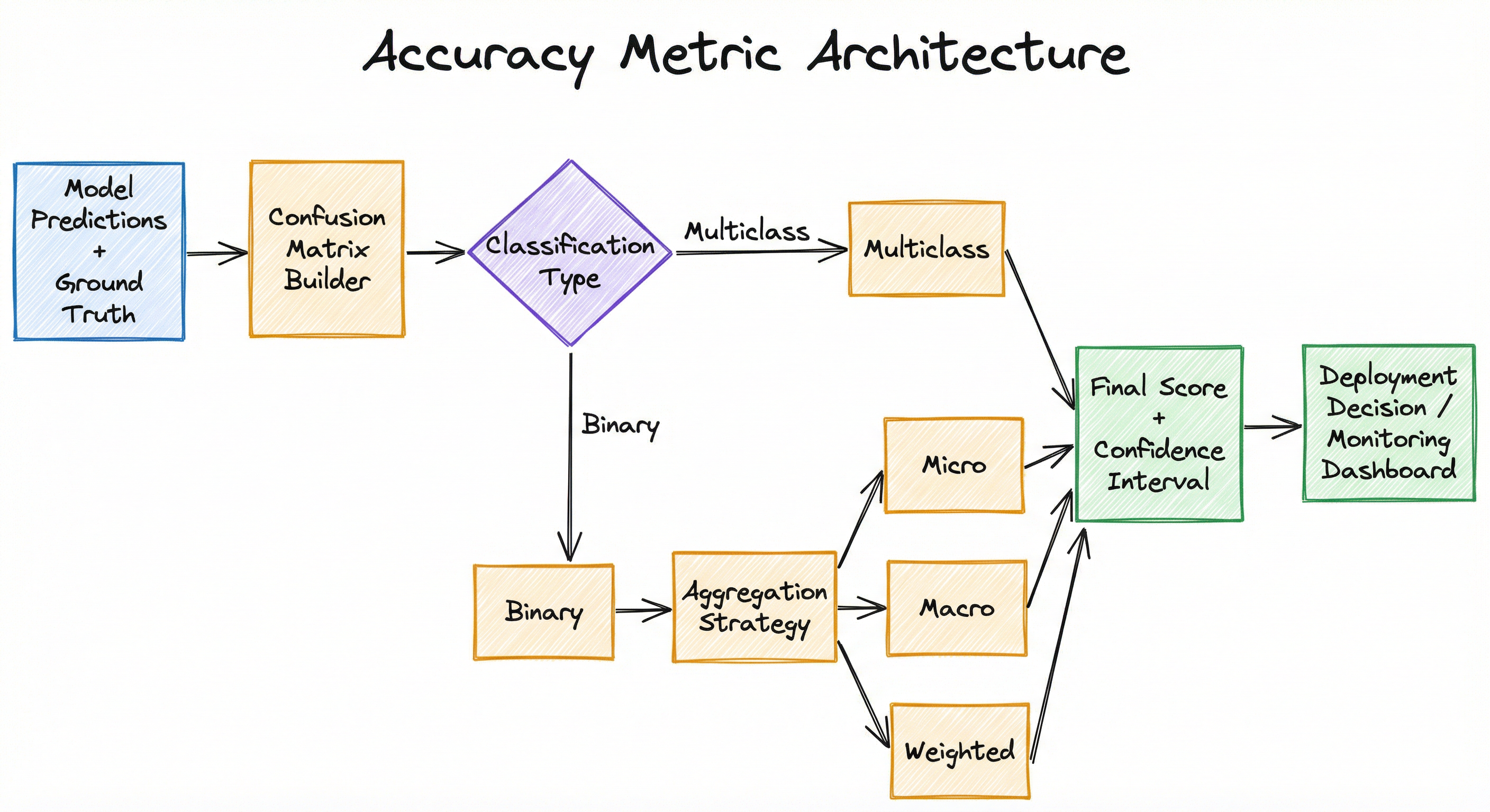
Internal Architecture
An accuracy computation system has three logical components: a prediction collector that gathers model predictions and ground truth labels for a test set, a confusion matrix builder that counts true positives, true negatives, false positives, and false negatives (or the multiclass generalization), and a metric aggregator that computes the final accuracy score using the appropriate averaging strategy (micro, macro, or weighted) and optionally confidence intervals via bootstrapping.
The architecture must handle both binary and multiclass problems, support different averaging strategies, and provide breakdown by class for diagnostic purposes. For production monitoring, the system typically includes a drift detector that tracks whether accuracy degrades over time as data distributions shift.
For imbalanced datasets, the architecture typically computes both standard accuracy and balanced accuracy, allowing practitioners to see the difference and make informed decisions.
Key Components
Prediction Collector
Gathers predicted labels and ground truth labels for the evaluation set. Ensures alignment (same sample IDs, same ordering) and handles missing values. In streaming production systems, this component buffers predictions and labels over a time window (e.g., 1 hour, 24 hours) to compute accuracy periodically.
Confusion Matrix Builder
Computes the confusion matrix for binary classification (2x2 matrix of TP, TN, FP, FN) or multiclass classification (KxK matrix). This is the foundational data structure from which accuracy and all other classification metrics are derived. The builder validates that predictions and labels use the same label set and handles edge cases like a class that never appears in the test set.
Metric Aggregator
Computes accuracy using the specified averaging strategy. For micro-averaging (default), sums all correct predictions and divides by total samples. For macro-averaging (balanced accuracy), computes per-class recall and averages. For weighted-averaging, weights per-class recall by class frequency. Returns the final score and optionally a confidence interval via bootstrap resampling.
Class-Specific Breakdown
Provides per-class accuracy (recall) alongside the overall score. Essential for diagnosing where the model succeeds and fails -- e.g., 95% accuracy on class A but 60% on class B indicates a problem even if overall accuracy is 90%. This breakdown is critical for fairness analysis and debugging class imbalance issues.
Drift Detector (Production)
Monitors accuracy over time in production systems. Computes accuracy on recent windows (e.g., daily batches) and compares to historical baseline. Alerts when accuracy drops below a threshold, indicating data distribution shift, model staleness, or upstream pipeline issues. Used extensively at Swiggy, Flipkart, and Razorpay to catch performance degradation before it impacts business KPIs.
Data Flow
Collection Phase: Model generates predictions on the test set or a live stream of production data. The prediction collector aligns predictions with ground truth labels (which may arrive with a delay in production -- e.g., fraud labels confirmed 24 hours later).
Matrix Phase: The confusion matrix builder counts TP, TN, FP, FN for binary problems or the full KxK matrix for multiclass. This step validates label consistency and handles edge cases (e.g., a predicted class that never appeared in training).
Aggregation Phase: The metric aggregator applies the chosen averaging strategy. Micro-averaging computes (ΣTP) / (ΣTP + ΣFN) across all classes, yielding standard accuracy. Macro-averaging computes per-class recall and takes the unweighted mean, yielding balanced accuracy. Weighted-averaging weights per-class recall by class frequency, which is mathematically equivalent to micro-averaging for accuracy.
Output Phase: The system returns the final accuracy score, per-class breakdown, and optionally a confidence interval (computed via bootstrap resampling: repeatedly sample the test set with replacement, compute accuracy on each sample, report the 95% CI). This output feeds into model selection decisions, deployment approvals, or production monitoring dashboards.
A vertical flow starting from 'Model Predictions + Ground Truth' feeding into 'Confusion Matrix Builder', which branches based on 'Classification Type' (Binary or Multiclass). Binary path computes '(TP+TN)/(TP+TN+FP+FN)', multiclass computes 'Σ Correct / Total'. Both feed into 'Aggregation Strategy', which branches to three paths: 'Micro' (Overall Accuracy), 'Macro' (Balanced Accuracy), and 'Weighted' (Class-Frequency Weighted). All three converge to 'Final Score + Confidence Interval', which flows to 'Deployment Decision / Monitoring Dashboard'.
How to Implement
Implementation Approaches
Accuracy computation is trivial in scikit-learn (accuracy_score) and all major ML frameworks. The challenge is not how to compute it, but when to use it and how to interpret it in the context of class imbalance and cost asymmetry.
Option A: Standard accuracy via sklearn.metrics.accuracy_score -- the default. Use this for balanced datasets (class ratio within 40:60 to 60:40) with symmetric costs. Reports a single number between 0 and 1.
Option B: Balanced accuracy via sklearn.metrics.balanced_accuracy_score -- computes the average of per-class recall. Use this for imbalanced datasets (class ratio outside 40:60 range). Gives equal weight to all classes regardless of frequency.
Option C: Stratified accuracy -- compute accuracy separately for each class (equivalent to per-class recall) and report alongside overall accuracy. This diagnostic view reveals where the model succeeds and fails.
Option D: Cost-weighted accuracy -- manually weight the confusion matrix elements by business costs (e.g., false negatives cost 100x more than false positives) and optimize a custom metric. This is the gold standard for production systems with known cost structures.
Cost Note: Accuracy computation itself is free -- it's a simple count operation. The cost comes from choosing the wrong metric and deploying a model that looks good on accuracy but performs poorly on what you actually care about. At Razorpay, switching from accuracy to F1-score for fraud detection reduced false negative rate by 40% at the cost of only 5% more false positives -- a tradeoff that saved millions in prevented fraud.
from sklearn.metrics import accuracy_score, balanced_accuracy_score, classification_report
from sklearn.model_selection import train_test_split
from sklearn.ensemble import RandomForestClassifier
import numpy as np

# Simulate imbalanced data (5% positive class)
np.random.seed(42)
X = np.random.randn(1000, 20)
y = (np.random.rand(1000) < 0.05).astype(int)  # 5% positive class

X_train, X_test, y_train, y_test = train_test_split(X, y, test_size=0.2, stratify=y, random_state=42)

model = RandomForestClassifier(n_estimators=100, random_state=42)
model.fit(X_train, y_train)
y_pred = model.predict(X_test)

# Standard accuracy
acc = accuracy_score(y_test, y_pred)
print(f"Accuracy: {acc:.4f}")  # Often high even for bad models on imbalanced data

# Balanced accuracy (better for imbalanced data)
bal_acc = balanced_accuracy_score(y_test, y_pred)
print(f"Balanced Accuracy: {bal_acc:.4f}")

# Full classification report (includes precision, recall, F1 per class)
print("\nClassification Report:")
print(classification_report(y_test, y_pred, target_names=['Negative', 'Positive']))

# Dummy classifier baseline (always predict majority class)
from sklearn.dummy import DummyClassifier
dummy = DummyClassifier(strategy='most_frequent')
dummy.fit(X_train, y_train)
y_dummy = dummy.predict(X_test)
print(f"\nDummy Classifier (always predict 0): {accuracy_score(y_test, y_dummy):.4f}")
# ^ This will be ~0.95 due to class imbalance, showing the accuracy paradox
This example demonstrates the accuracy paradox: on a dataset with 5% positive class, a dummy classifier that always predicts negative achieves ~95% accuracy. The actual model might achieve 96% accuracy, appearing only marginally better, while its balanced accuracy (or F1 score) reveals the true performance gap. Always compare against a baseline, and use balanced accuracy for imbalanced data.
from sklearn.metrics import accuracy_score, recall_score, precision_score, f1_score
from sklearn.datasets import make_classification
from sklearn.ensemble import GradientBoostingClassifier
import numpy as np

# Simulate multiclass imbalanced data (3 classes with different frequencies)
X, y = make_classification(
    n_samples=1000, n_features=20, n_informative=15, n_redundant=5,
    n_classes=3, n_clusters_per_class=1,
    weights=[0.7, 0.2, 0.1],  # Imbalanced: 70% class 0, 20% class 1, 10% class 2
    random_state=42
)

model = GradientBoostingClassifier(n_estimators=100, random_state=42)
model.fit(X[:800], y[:800])
y_pred = model.predict(X[800:])
y_test = y[800:]

# Standard accuracy (micro-averaged)
acc_micro = accuracy_score(y_test, y_pred)
print(f"Accuracy (micro): {acc_micro:.4f}")

# Macro-averaged accuracy (balanced accuracy)
acc_macro = recall_score(y_test, y_pred, average='macro')
print(f"Accuracy (macro/balanced): {acc_macro:.4f}")

# Weighted-averaged accuracy (weighted by class frequency)
acc_weighted = recall_score(y_test, y_pred, average='weighted')
print(f"Accuracy (weighted): {acc_weighted:.4f}")

# Per-class accuracy (recall)
per_class_recall = recall_score(y_test, y_pred, average=None)
for i, recall in enumerate(per_class_recall):
    count = np.sum(y_test == i)
    print(f"Class {i} accuracy (recall): {recall:.4f} ({count} samples)")

# Key insight: macro gives equal weight to all classes, weighted aligns with overall accuracy
print(f"\nMicro ≈ Weighted: {np.isclose(acc_micro, acc_weighted)}")
For multiclass classification, micro-averaging (standard accuracy) is dominated by large classes, macro-averaging (balanced accuracy) treats all classes equally, and weighted-averaging weights by class frequency (equivalent to micro for accuracy). Use macro when all classes are equally important; use weighted when class frequencies reflect real-world importance. The per-class breakdown reveals which classes the model struggles with.
from sklearn.metrics import accuracy_score
from sklearn.utils import resample
import numpy as np

def accuracy_with_confidence_interval(y_true, y_pred, n_iterations=1000, ci=95):
    """
    Compute accuracy with bootstrap confidence interval.

    Returns:
        accuracy: float, point estimate
        ci_lower: float, lower bound of confidence interval
        ci_upper: float, upper bound of confidence interval
    """
    n = len(y_true)
    accuracies = []

    for _ in range(n_iterations):
        # Bootstrap resample
        indices = resample(range(n), n_samples=n, random_state=None)
        y_true_boot = [y_true[i] for i in indices]
        y_pred_boot = [y_pred[i] for i in indices]

        # Compute accuracy on bootstrap sample
        acc = accuracy_score(y_true_boot, y_pred_boot)
        accuracies.append(acc)

    # Compute percentiles for confidence interval
    alpha = (100 - ci) / 2
    ci_lower = np.percentile(accuracies, alpha)
    ci_upper = np.percentile(accuracies, 100 - alpha)

    accuracy = accuracy_score(y_true, y_pred)
    return accuracy, ci_lower, ci_upper

# Example usage
np.random.seed(42)
y_true = np.random.randint(0, 2, 200)
y_pred = np.random.randint(0, 2, 200)

acc, ci_low, ci_high = accuracy_with_confidence_interval(y_true, y_pred, n_iterations=1000, ci=95)
print(f"Accuracy: {acc:.4f} [95% CI: {ci_low:.4f} - {ci_high:.4f}]")

# If confidence interval is wide, you need more test data or repeated CV
ci_width = ci_high - ci_low
print(f"CI width: {ci_width:.4f}")
if ci_width > 0.05:
    print("Warning: Wide confidence interval. Consider collecting more test data.")
Bootstrap resampling provides a confidence interval on accuracy, revealing the uncertainty in your estimate. A wide CI (>5 percentage points) indicates high variance -- your test set is too small or your model's performance is unstable. For production deployment decisions, always report accuracy with confidence intervals to quantify uncertainty. This is critical for comparing two models: if their CIs overlap significantly, the difference may not be statistically meaningful.
from sklearn.metrics import confusion_matrix, classification_report
import numpy as np
import pandas as pd

def stratified_accuracy_analysis(y_true, y_pred, class_names=None):
    """
    Compute overall accuracy, per-class accuracy, and balanced accuracy.
    Show where the model succeeds and fails.
    """
    cm = confusion_matrix(y_true, y_pred)
    n_classes = cm.shape[0]

    if class_names is None:
        class_names = [f"Class {i}" for i in range(n_classes)]

    # Overall accuracy
    overall_acc = np.trace(cm) / np.sum(cm)

    # Per-class accuracy (recall)
    per_class_acc = cm.diagonal() / cm.sum(axis=1)

    # Balanced accuracy (macro-averaged recall)
    balanced_acc = np.mean(per_class_acc)

    # Class frequencies
    class_freq = cm.sum(axis=1) / np.sum(cm)

    # Build summary table
    summary = pd.DataFrame({
        'Class': class_names,
        'Samples': cm.sum(axis=1),
        'Frequency': class_freq,
        'Accuracy (Recall)': per_class_acc,
        'Contribution to Overall': per_class_acc * class_freq
    })

    print(f"Overall Accuracy: {overall_acc:.4f}")
    print(f"Balanced Accuracy: {balanced_acc:.4f}")
    print(f"Gap (Overall - Balanced): {overall_acc - balanced_acc:+.4f}")
    print("\nPer-Class Breakdown:")
    print(summary.to_string(index=False))

    # Flag classes with low accuracy
    threshold = 0.7
    struggling_classes = summary[summary['Accuracy (Recall)'] < threshold]
    if not struggling_classes.empty:
        print(f"\nClasses with <{threshold*100:.0f}% accuracy:")
        print(struggling_classes[['Class', 'Accuracy (Recall)']].to_string(index=False))

    return overall_acc, balanced_acc, summary

# Example: Fraud detection (1% fraud rate)
np.random.seed(42)
n_samples = 1000
y_true = (np.random.rand(n_samples) < 0.01).astype(int)  # 1% fraud
# Simulate a model that's good at detecting non-fraud, poor at detecting fraud
y_pred = y_true.copy()
y_pred[y_true == 1] = np.random.rand(np.sum(y_true == 1)) > 0.4  # Only catches 60% of fraud

overall, balanced, summary = stratified_accuracy_analysis(
    y_true, y_pred, class_names=['Legitimate', 'Fraud']
)
This function reveals the class imbalance problem by showing how overall accuracy and balanced accuracy diverge. A model with 99% overall accuracy might have only 60% accuracy on the minority class (fraud), but overall accuracy masks this because the minority class contributes little to the total. The per-class breakdown and contribution analysis show exactly where the model fails. Use this pattern for all production classification systems to diagnose performance disparities across classes.
from sklearn.metrics import confusion_matrix
import numpy as np

def cost_sensitive_accuracy(y_true, y_pred_proba, threshold=0.5, cost_matrix=None):
    """
    Compute accuracy accounting for asymmetric misclassification costs.

    cost_matrix: 2x2 array where cost_matrix[i, j] is the cost of
                 predicting class j when true class is i.
                 Default: [[0, 1], [10, 0]] (FN costs 10x FP)
    """
    if cost_matrix is None:
        # Default: False Negative costs 10x more than False Positive
        cost_matrix = np.array([
            [0, 1],    # TN cost 0, FP cost 1
            [10, 0]    # FN cost 10, TP cost 0
        ])

    # Apply threshold to probabilities
    y_pred = (y_pred_proba >= threshold).astype(int)

    # Compute confusion matrix
    cm = confusion_matrix(y_true, y_pred)
    tn, fp, fn, tp = cm.ravel()

    # Standard accuracy
    accuracy = (tp + tn) / (tp + tn + fp + fn)

    # Cost-sensitive score (lower is better, we want to minimize cost)
    total_cost = (
        cost_matrix[0, 0] * tn +
        cost_matrix[0, 1] * fp +
        cost_matrix[1, 0] * fn +
        cost_matrix[1, 1] * tp
    )

    # Normalize cost to [0, 1] range (cost-weighted accuracy)
    # Maximum cost: all samples misclassified with worst-case cost
    max_cost_per_sample = max(cost_matrix[0, 1], cost_matrix[1, 0])
    max_total_cost = max_cost_per_sample * len(y_true)
    cost_weighted_accuracy = 1 - (total_cost / max_total_cost)

    return {
        'threshold': threshold,
        'accuracy': accuracy,
        'cost_weighted_accuracy': cost_weighted_accuracy,
        'total_cost': total_cost,
        'confusion': {'TP': tp, 'TN': tn, 'FP': fp, 'FN': fn}
    }

def find_optimal_threshold(y_true, y_pred_proba, cost_matrix=None, thresholds=None):
    """
    Find the threshold that maximizes cost-weighted accuracy.
    """
    if thresholds is None:
        thresholds = np.linspace(0.1, 0.9, 50)

    results = [cost_sensitive_accuracy(y_true, y_pred_proba, t, cost_matrix) for t in thresholds]

    # Find threshold that maximizes cost-weighted accuracy (minimizes cost)
    best_idx = np.argmax([r['cost_weighted_accuracy'] for r in results])
    best = results[best_idx]

    print(f"Optimal Threshold: {best['threshold']:.3f}")
    print(f"Standard Accuracy: {best['accuracy']:.4f}")
    print(f"Cost-Weighted Accuracy: {best['cost_weighted_accuracy']:.4f}")
    print(f"Total Cost: {best['total_cost']:.0f}")
    print(f"Confusion Matrix: TP={best['confusion']['TP']}, TN={best['confusion']['TN']}, "
          f"FP={best['confusion']['FP']}, FN={best['confusion']['FN']}")

    return best['threshold'], results

# Example: Fraud detection where FN (missing fraud) costs 100x more than FP
np.random.seed(42)
n_samples = 1000
y_true = (np.random.rand(n_samples) < 0.01).astype(int)  # 1% fraud
# Simulate predicted probabilities (model has some signal)
y_pred_proba = np.random.beta(1 + y_true * 3, 5 - y_true * 3)

cost_matrix_fraud = np.array([
    [0, 1],      # TN cost 0, FP cost 1 (manual review)
    [100, 0]     # FN cost 100 (fraud loss), TP cost 0
])

optimal_thresh, results = find_optimal_threshold(y_true, y_pred_proba, cost_matrix_fraud)
This example shows how to move beyond accuracy to cost-sensitive evaluation. When false negatives (missing fraud) cost 100x more than false positives (flagging legitimate transactions), the optimal threshold is NOT 0.5. By sweeping thresholds and computing cost-weighted accuracy, you find the threshold that minimizes business cost. At Razorpay, PhonePe, and other fintech companies, this threshold optimization is critical -- it directly translates to millions in prevented fraud losses vs. customer friction from false positives.
# Model evaluation configuration (YAML)
evaluation:
  metrics:
    primary: balanced_accuracy  # Use balanced accuracy for imbalanced data
    additional:
      - accuracy               # Report standard accuracy for reference
      - precision_weighted     # Weighted precision
      - recall_weighted        # Weighted recall
      - f1_weighted            # Weighted F1
      - roc_auc               # Threshold-independent metric

  class_imbalance_handling:
    strategy: stratified         # Stratify train/test split by class
    use_balanced_accuracy: true  # Use balanced accuracy as primary metric
    report_per_class: true       # Report per-class metrics

  baseline_comparison:
    enabled: true
    baselines:
      - type: majority_class
        description: "Always predict most frequent class"
      - type: stratified_random
        description: "Random predictions matching class distribution"
      - type: rule_based
        description: "Simple if-then rules from domain experts"

  cost_matrix:                 # For cost-sensitive evaluation
    # Rows: true class, Columns: predicted class
    # cost_matrix[i][j] = cost of predicting j when truth is i
    enabled: true
    matrix:
      - [0, 1]      # TN cost 0, FP cost 1 (manual review ₹100)
      - [100, 0]    # FN cost 100 (fraud loss ₹10,000), TP cost 0

  threshold_optimization:
    enabled: true
    metric: cost_weighted_accuracy
    search_range: [0.05, 0.95]
    search_steps: 50

  confidence_intervals:
    enabled: true
    method: bootstrap
    n_iterations: 1000
    confidence_level: 95

  monitoring:                  # Production monitoring
    track_over_time: true
    window_size: 24h
    alert_threshold: 0.05      # Alert if accuracy drops >5%
    compare_to_baseline: validation_set
Common Implementation Mistakes
- ●
Using accuracy on imbalanced data: With 1% fraud rate, a model that predicts 'not fraud' for everything achieves 99% accuracy but is useless. Always use balanced accuracy, F1, or AUC-ROC for imbalanced problems, and compare against a majority-class baseline.
- ●
Ignoring per-class accuracy: Overall accuracy can be high while minority class accuracy is terrible. Always report per-class recall alongside overall accuracy to reveal performance disparities across classes.
- ●
Confusing accuracy with precision: Accuracy measures overall correctness; precision measures correctness among positive predictions. For rare-event detection (spam, fraud, disease), precision tells you what fraction of your alerts are real, while accuracy just tells you how often you're right overall.
- ●
Not considering cost asymmetry: In production, false positives and false negatives have different costs. Optimizing accuracy assumes equal costs. Define a business metric that incorporates actual costs (e.g., FN costs ₹10,000, FP costs ₹100) and optimize that instead.
- ●
Reporting accuracy without a baseline: 85% accuracy sounds good until you realize a trivial baseline (always predict the majority class) achieves 82%. Always compare against baselines: stratified random guessing, majority class, or a simple rule-based system.
- ●
Using accuracy for threshold selection: Accuracy is maximized at threshold ~0.5 for balanced data, but the optimal threshold for business outcomes may be very different (0.2 or 0.8). Use cost-sensitive metrics or ROC analysis for threshold selection, not accuracy.
When Should You Use This?
Use When
Your dataset has balanced classes (class ratios within 40:60 to 60:40 range) and all classes are equally important to the business
Misclassification costs are symmetric -- false positives and false negatives have roughly equal business impact
You need a simple, interpretable metric for non-technical stakeholders who understand 'percentage correct' intuitively
You are working on a well-understood benchmark dataset (MNIST, CIFAR-10, ImageNet) where accuracy is the standard metric for comparison
All classes have sufficient representation in the test set (at least 30-50 samples per class) to make per-class accuracy estimates reliable
You are doing rapid prototyping and need a quick sanity-check metric before investing in more sophisticated evaluation
Avoid When
Your dataset is imbalanced (class ratio outside 40:60 range) -- use balanced accuracy, F1, AUC-ROC, or PR-AUC instead to avoid the accuracy paradox
Misclassification costs are asymmetric -- missing a fraud transaction costs 100x more than flagging a legitimate one for review. Use cost-sensitive metrics that incorporate actual business costs
You care more about one class than others (e.g., in medical diagnosis, detecting disease is more important than correctly identifying healthy patients) -- use precision, recall, or F1 for the class of interest
The minority class is extremely rare (<1% prevalence) and critical -- a model that ignores the minority class entirely can still achieve high accuracy. Use PR-AUC or balanced accuracy
Your test set has very few samples from some classes (<10 samples) -- accuracy estimates will have high variance and be unreliable
You need to compare models and the expected performance difference is small (1-2%) -- accuracy variance may obscure real differences. Use repeated cross-validation with statistical testing
Key Tradeoffs
Interpretability vs. Robustness
Accuracy's greatest strength is its interpretability: '92% correct' is immediately meaningful to anyone. Its greatest weakness is lack of robustness to class imbalance: it can be high even when the model fails on what matters.
Balanced accuracy trades interpretability for robustness. Saying 'balanced accuracy is 0.78' requires explaining that it's the average of per-class recall, which is less intuitive. But it correctly penalizes models that ignore minority classes.
Single Metric vs. Metric Portfolio
Accuracy provides a single number for ranking models. This simplicity is valuable when you need to make quick decisions or report to stakeholders who want a simple answer. But a single number obscures important details.
A metric portfolio (accuracy + precision + recall + F1 + AUC) provides a multidimensional view of performance. You might have high accuracy but low precision on the minority class, indicating the model is good overall but struggles with rare events. The tradeoff is complexity: which metric do you optimize? How do you compare two models when one wins on accuracy and the other on F1?
Overall vs. Per-Class Accuracy
Overall accuracy weights all samples equally. Per-class accuracy (recall) weights all classes equally. For balanced datasets, these are similar. For imbalanced datasets, they diverge dramatically.
| Scenario | Overall Accuracy | Balanced Accuracy | Best Choice |
|---|---|---|---|
| Balanced data (50:50) | 0.90 | 0.90 | Either |
| Imbalanced data (90:10), model ignores minority | 0.90 | 0.50 | Balanced |
| Imbalanced data (90:10), model is good at both | 0.90 | 0.85 | Both |
| Cost-sensitive (FN >> FP) | Not applicable | Not applicable | Custom cost metric |
Threshold-Dependent vs. Threshold-Independent
Accuracy is threshold-dependent: it requires converting predicted probabilities to hard labels using a threshold (default 0.5). Changing the threshold changes accuracy. This means accuracy is not a pure measure of model quality -- it confounds model quality with threshold choice.
AUC-ROC is threshold-independent: it measures how well the model ranks positive samples above negative samples across all thresholds. This makes AUC a purer measure of model discrimination ability, but it's less interpretable and doesn't tell you what performance to expect at a specific operating point.
Practical recommendation: Report both. Use AUC-ROC to compare models (which one has better discrimination?). Use accuracy, precision, and recall at a chosen threshold to estimate production performance (what will I see when I deploy?).
Alternatives & Comparisons
Precision and recall decompose accuracy into class-specific metrics: precision measures correctness among positive predictions, recall measures coverage of actual positives. F1 is their harmonic mean. Use precision/recall/F1 when classes are imbalanced or when you care more about one class than others. Accuracy is simpler and better for balanced data with symmetric costs.
AUC-ROC is threshold-independent and measures how well the model ranks positive samples above negative samples across all thresholds. It's robust to class imbalance and better for model comparison. Accuracy is threshold-dependent (requires choosing a cutoff) and easier to interpret for stakeholders. Use AUC for model selection, accuracy for reporting deployment performance.
A confusion matrix provides the raw counts (TP, TN, FP, FN) from which accuracy and all other metrics are derived. It's more informative than accuracy alone because it shows where errors occur. Accuracy is a single-number summary of the confusion matrix. Always visualize the confusion matrix alongside accuracy to understand error patterns.
Cohen's Kappa adjusts accuracy for the expected agreement by chance, making it more informative for imbalanced data. It ranges from -1 to 1, where 0 is random agreement and 1 is perfect agreement. Kappa is better than accuracy for imbalanced data, but less intuitive. Use Kappa when you need a chance-corrected metric; use accuracy for simplicity.
Pros, Cons & Tradeoffs
Advantages
Maximum interpretability -- '85% accurate' is instantly understood by anyone, from data scientists to executives to customers. No other metric is as universally comprehensible
Simple to compute -- a single division: (correct predictions) / (total predictions). No need for probability calibration, threshold tuning, or complex aggregations
Well-established baseline -- decades of research and benchmarks use accuracy, making it easy to compare your model to published results and industry standards
Appropriate for balanced data -- when classes are equally represented and errors are equally costly, accuracy is a perfectly reasonable metric that balances precision and recall naturally
Default in most frameworks -- scikit-learn, TensorFlow, PyTorch all default to accuracy for classification, making it the path of least resistance for quick prototyping
Aligns with intuitive correctness -- stakeholders naturally think 'how often is the model right?' rather than 'what's the harmonic mean of precision and recall?'
Disadvantages
Misleading on imbalanced data -- the accuracy paradox: with 1% fraud rate, predicting 'not fraud' for everything gives 99% accuracy but is completely useless. This is not a theoretical concern; it's the most common failure mode in production ML
Ignores cost asymmetry -- treats false positives and false negatives as equally bad, but in reality, missing a ₹50,000 fraud (FN) costs far more than flagging a ₹500 legitimate transaction for review (FP). Accuracy cannot capture business costs
Hides minority class failure -- a model can have 95% overall accuracy while having only 40% accuracy on the minority class (the class you actually care about). Per-class breakdown is essential but accuracy alone obscures this
Threshold-dependent -- accuracy changes with the classification threshold. A model with 90% accuracy at threshold 0.5 might have 85% at 0.3 or 95% at 0.7. This confounds model quality with threshold choice
Not robust to distribution shift -- if the class distribution changes in production (e.g., fraud rate increases from 1% to 3%), accuracy will drop even if model discrimination ability is unchanged. Threshold-independent metrics like AUC are more stable
Prevents proper model comparison -- when comparing two models on imbalanced data, the one with higher accuracy is not necessarily better at the task. Use F1, AUC, or balanced accuracy for fair comparison
Failure Modes & Debugging
Accuracy Paradox on Imbalanced Data
Cause
Using accuracy as the primary metric on a dataset with severe class imbalance (e.g., 1% fraud, 99% legitimate). The model learns to predict the majority class for everything because that maximizes accuracy.
Symptoms
Model reports 98-99% accuracy but catches almost no fraud (0-20% recall on minority class). In production, fraud losses remain unchanged despite 'high accuracy.' The confusion matrix shows TP ≈ 0 and FN ≈ (all minority samples), but TN is huge, making accuracy high.
Mitigation
Switch to balanced accuracy or F1 score as the primary metric. Report per-class recall alongside overall accuracy. Compare against a majority-class baseline -- if the model barely beats the baseline, it's not learning. For fraud detection at Razorpay-like systems, use PR-AUC (precision-recall AUC) which is robust to extreme imbalance and focuses on the minority class performance.
Ignoring Cost Asymmetry
Cause
Optimizing accuracy when false negatives and false positives have drastically different business costs. The model balances errors to maximize accuracy, but this balance is economically wrong.
Symptoms
High accuracy in evaluation, but poor business outcomes in production. For example, a medical diagnostic model with 92% accuracy might miss 30% of cancer cases (false negatives) to avoid false alarms (false positives), but missing cancer is far worse than an extra test. Business metrics (revenue, customer satisfaction, regulatory fines) diverge from model accuracy.
Mitigation
Define a cost matrix where cost[i,j] = cost of predicting class j when truth is class i. Compute cost-weighted accuracy or expected cost. Tune the classification threshold to minimize expected cost, not maximize accuracy. At PhonePe and other fintech platforms, false negatives (fraud) cost 100-1000x more than false positives (manual review), so thresholds are set to 0.1-0.3, not 0.5, to catch more fraud at the cost of more alerts.
Threshold Misalignment
Cause
Using the default threshold of 0.5 to convert probabilities to hard labels, then reporting accuracy. The default threshold is optimal only for balanced data with symmetric costs. For imbalanced or cost-sensitive problems, 0.5 is almost always wrong.
Symptoms
Model has good discrimination ability (high AUC-ROC) but poor accuracy because the threshold is misaligned with the operating point. Alternatively, accuracy is high at the wrong threshold, leading to poor production performance when deployed at the default threshold.
Mitigation
Perform threshold optimization by sweeping thresholds from 0.1 to 0.9 and computing accuracy (or better, cost-weighted accuracy) at each point. Plot accuracy vs. threshold to visualize the tradeoff. Choose the threshold that maximizes business value, not accuracy. Report accuracy at the chosen threshold alongside AUC-ROC. Use scikit-learn's TunedThresholdClassifierCV for automated threshold tuning based on a custom metric.
Data Distribution Shift
Cause
The test set has a different class distribution than the training set or production data. Model accuracy on the test set does not reflect production performance because the base rate has shifted.
Symptoms
Model achieves 88% accuracy in offline evaluation but only 70% in production. Monitoring dashboards show accuracy degrading over time as the data distribution drifts (e.g., fraud tactics evolve, seasonal patterns change, user behavior shifts).
Mitigation
Ensure the test set is stratified to match the expected production distribution. For time-series data, use time-based splits (train on past, test on future) to simulate deployment conditions. Monitor accuracy in production over rolling windows (daily, weekly) and alert when it drops below a threshold. At Swiggy, delivery time prediction models are retrained weekly because distribution shifts (festivals, weather, new restaurant openings) cause accuracy to degrade. Use threshold-independent metrics like AUC-ROC for model comparison since they're more robust to distribution shift.
Insufficient Test Set Size for Minority Class
Cause
The test set has very few samples from the minority class (e.g., 5 fraud samples out of 500 total). Accuracy on the minority class has high variance and is unreliable.
Symptoms
Per-class accuracy for the minority class swings wildly between test sets or cross-validation folds (40% in one fold, 80% in another). Confidence intervals on minority class accuracy are extremely wide (±20 percentage points).
Mitigation
Use stratified sampling to ensure sufficient representation of all classes in the test set (aim for at least 30-50 samples per class). If the minority class is too rare, use stratified K-fold cross-validation (K=5 or K=10) to aggregate performance across folds, reducing variance. Report confidence intervals on accuracy via bootstrap resampling. For extremely rare events (<0.1% prevalence), consider collecting more labeled data specifically for the minority class or using synthetic oversampling (SMOTE) during training (but never during testing!).
Placement in an ML System
Where Does It Sit in the Pipeline?
Accuracy sits at the evaluation stage of the ML pipeline, after model training and before deployment. It operates on a held-out test set (or cross-validation folds) to estimate how the model will perform on unseen data.
The typical workflow is: data collection -> preprocessing -> train/test split -> model training -> accuracy evaluation -> model selection -> hyperparameter tuning -> final training -> test set accuracy -> deploy -> production accuracy monitoring.
Notice accuracy appears three times: (1) during development for model comparison, (2) on the final test set for deployment decision, and (3) in production for monitoring degradation. Each serves a different purpose.
Development Accuracy: Used to compare multiple models or hyperparameter configurations. Computed on validation sets or via cross-validation. Guides model selection decisions. Here, balanced accuracy or F1 may be more appropriate than standard accuracy for imbalanced data.
Test Set Accuracy: Computed once on a held-out test set that was never used during development. This is the unbiased estimate of deployment performance. Reported alongside confidence intervals to quantify uncertainty. This is the number that goes into the model registry and deployment documentation.
Production Accuracy: Computed continuously on live data as ground truth labels arrive (often with delay). Monitors for distribution shift, model staleness, or upstream pipeline issues. Triggers alerts when accuracy drops below a threshold, prompting retraining or incident response.
Key Insight: Accuracy is not a one-time number -- it's a continuous monitoring signal in production ML systems. The initial test set accuracy is a prediction of production accuracy. When production accuracy diverges from test accuracy, it indicates distribution shift, data quality issues, or changes in user behavior. At Swiggy and Flipkart, production accuracy is tracked on dashboards alongside business KPIs (delivery time, conversion rate) to provide early warning of model degradation.
Pipeline Stage
Evaluation / Model Selection
Upstream
- model-training
- train-test-split
- cross-validation
Downstream
- model-registry
- deployment
- monitoring
Scaling Bottlenecks
Accuracy computation itself is trivial -- it's a single O(n) pass over predictions. The cost comes from collecting ground truth labels in production, which may require human annotation, delayed feedback (fraud confirmed 24 hours later), or expensive verification processes.
For batch systems (offline model evaluation), accuracy is free. You have ground truth labels for the test set, compute predictions once, calculate accuracy in milliseconds.
For online systems (production monitoring), getting labels is expensive. At Razorpay, fraud labels arrive with 1-24 hour delays after transactions are confirmed. At Swiggy, delivery time accuracy can only be computed after the order is completed (30-60 minutes later). This means production accuracy monitoring operates on delayed batches, not real-time streams.
The annotation cost for ground truth can be substantial. Medical diagnosis requires expert radiologists (₹5,000-10,000 per hour in India). Content moderation requires trained reviewers (₹500-1,000 per hour for quality-controlled labeling). For large-scale systems, this can be millions in annual labeling costs.
Another scaling bottleneck is stratified evaluation. To compute per-class accuracy reliably, you need sufficient samples from each class. For a rare class (<0.1% prevalence), you might need 100,000 total samples to get 100 rare-class samples for evaluation. This drives up data collection and storage costs.
At Indian ML teams (Flipkart, Swiggy, Razorpay), the tradeoff is between evaluation rigor and iteration speed. Rigorous evaluation (stratified cross-validation, balanced accuracy, confidence intervals, per-class breakdown) takes more compute and more labeled data but prevents costly deployment mistakes. Lightweight evaluation (single holdout, accuracy only) is faster but risks deploying models with hidden failure modes.
The pragmatic approach: use lightweight evaluation for rapid prototyping (hundreds of experiments), then invest in rigorous evaluation for final model selection (5-10 finalists). This 100:1 funnel balances speed and safety.
Production Case Studies
Swiggy's demand forecasting system for Instamart uses multiple accuracy metrics adapted to different business contexts. For high-demand items, they optimize for overall accuracy to ensure inventory availability. For long-tail items with sparse demand, they use balanced accuracy to avoid ignoring rare but important products. The team implemented adaptive metric alignment where the evaluation metric changes based on product category and demand pattern.
By using stratified accuracy evaluation (balanced accuracy for rare items, standard accuracy for popular items), Swiggy reduced stockouts for rare items by 30% while maintaining 95%+ accuracy on high-volume products. The system now evaluates 10,000+ SKUs daily with category-specific metrics, preventing the accuracy paradox that would have occurred with a one-size-fits-all metric.
PayPal's engineering blog details deploying large-scale fraud detection ML models using their Quokka shadow platform, processing millions of transactions daily with millisecond-level decision times using Gradient Boosting Machine models.
Model development and deployment time reduced by 80%, with data science team adoption growing at 50% quarter-over-quarter since launching the ML platform.
A systematic review of FDA-approved AI-enabled medical devices found that while many report high accuracy (>90%), the critical metric is balanced accuracy across patient subgroups (age, sex, ethnicity). A skin cancer detection AI achieved 94% overall accuracy but only 78% accuracy on darker skin tones due to class imbalance in training data. The study emphasizes that overall accuracy masks performance disparities that are clinically dangerous.
The FDA now requires stratified accuracy reporting for AI medical devices -- accuracy must be reported separately for demographic subgroups and disease subtypes. Devices with >10% accuracy gap between subgroups face additional scrutiny. This regulatory shift acknowledges that overall accuracy is insufficient for ensuring equitable healthcare outcomes, driving the adoption of balanced accuracy and subgroup-specific evaluation in medical AI.
Flipkart's address classification system uses ML to parse unstructured Indian addresses (which often lack standardized formatting) into structured components (city, locality, building). Initial models optimized for overall accuracy achieved 92% but performed poorly on rare localities and alternate spellings. The team switched to balanced accuracy to ensure all localities, regardless of frequency, were correctly classified.
By using balanced accuracy and per-locality evaluation, Flipkart improved rare-locality classification accuracy from 65% to 88% while maintaining 94% accuracy on common localities. The system now handles 10M+ addresses daily with hierarchical evaluation: overall accuracy for stakeholder reporting, balanced accuracy for model selection, and per-locality accuracy for debugging specific regions. This prevented delivery failures in underrepresented areas that would have been missed by accuracy-only evaluation.
Tooling & Ecosystem
The standard Python function for computing classification accuracy. Supports binary and multiclass classification, sample weighting, and normalization options. Use normalize=True (default) for accuracy as a proportion (0-1), or normalize=False for raw count of correct predictions. Part of sklearn.metrics module.
Computes balanced accuracy (macro-averaged recall) for binary and multiclass classification. Gives equal weight to all classes regardless of frequency, making it robust to class imbalance. Preferred over standard accuracy for imbalanced datasets. Returns a value between 0 and 1, where random guessing gives ~0.5.
Generates a comprehensive text report showing precision, recall, F1 score, and support for each class, plus overall accuracy, macro average, and weighted average. Essential for diagnosing model performance on imbalanced data -- reveals per-class accuracy that overall accuracy obscures. Supports JSON output for programmatic parsing.
Meta-estimator that tunes the decision threshold for binary classification to optimize a specified metric (accuracy, F1, cost-sensitive metric). Useful for finding the threshold that maximizes accuracy or business value instead of using the default 0.5. Performs cross-validated threshold search and refits the base estimator.
Open-source Python library for monitoring ML models in production. Tracks accuracy, precision, recall, and other metrics over time, detects data drift that causes accuracy degradation, and generates interactive dashboards. Compares production accuracy to reference (test set) accuracy to identify distribution shifts. Used by Swiggy, Razorpay-like systems for real-time model monitoring.
Experiment tracking and model monitoring platform that logs accuracy and other metrics across experiments. Provides visualization of accuracy vs. hyperparameters, comparison of accuracy across model versions, and production monitoring dashboards. Integrates with scikit-learn, TensorFlow, PyTorch. Commercial product with free tier.
Visualization library for scikit-learn that generates confusion matrix heatmaps and classification reports. Shows accuracy visually as the sum of diagonal elements. Highlights where errors occur, making it easy to diagnose class-specific accuracy problems. Essential for communicating accuracy results to non-technical stakeholders.
Research & References
Halligan, S., Altman, D. G., & Mallett, S. (2024)Scientific Reports, Vol. 14
Comprehensive survey of classification metrics including accuracy, balanced accuracy, sensitivity, specificity, and chance-corrected metrics (Cohen's Kappa, Matthews correlation coefficient). Emphasizes that accuracy is unreliable for imbalanced data and recommends balanced accuracy or class-specific metrics. Provides statistical tests for comparing classifiers and guidelines for choosing evaluation metrics based on problem characteristics.
Hossin, M., & Sulaiman, M. N. (2015)International Journal of Data Mining & Knowledge Management Process, Vol. 5, No. 2
Reviews evaluation metrics for classification tasks with focus on accuracy, precision, recall, F-measure, ROC curves, and their applications. Discusses the accuracy paradox and recommends alternatives for imbalanced datasets. Provides mathematical definitions and examples for each metric. Essential reading for understanding when accuracy is appropriate vs. when alternatives are needed.
Grandini, M., Bagli, E., & Visani, G. (2020)arXiv preprint
Comprehensive overview of multiclass classification metrics including micro, macro, and weighted averaging of accuracy, precision, recall, and F1. Explains when each averaging strategy is appropriate and how they behave under class imbalance. Provides Python code examples for all metrics. Critical for understanding the nuances of multiclass accuracy evaluation.
Saito, T., & Rehmsmeier, M. (2015)PLOS ONE, Vol. 10, No. 3
Demonstrates that accuracy and ROC-AUC can be misleading on highly imbalanced datasets, while precision-recall curves and PR-AUC are more informative. Shows that a classifier with 99% accuracy and 0.99 ROC-AUC can have only 0.5 PR-AUC, revealing poor minority class performance. Essential for fraud detection, medical diagnosis, and other rare-event classification tasks.
Elkan, C. (2001)Proceedings of IJCAI-01
Foundational paper on cost-sensitive learning showing that maximizing accuracy is optimal only when misclassification costs are equal and class distributions are balanced. Derives the optimal decision rule when costs are asymmetric and shows how to adjust classifiers via threshold tuning and cost-proportionate resampling. Essential for understanding when to move beyond accuracy to cost-weighted metrics.
Interview & Evaluation Perspective
Common Interview Questions
- ●
What is accuracy and how is it calculated for binary and multiclass classification?
- ●
What is the accuracy paradox and when does accuracy become misleading?
- ●
When would you use balanced accuracy instead of standard accuracy?
- ●
How do you handle accuracy evaluation on highly imbalanced datasets (e.g., 1% fraud rate)?
- ●
What's the difference between micro, macro, and weighted averaging for multiclass accuracy?
- ●
Why might a model with 95% accuracy still be bad in production?
- ●
How would you explain accuracy vs. precision vs. recall to a non-technical stakeholder?
- ●
What baseline would you compare against when reporting accuracy?
Key Points to Mention
- ●
The accuracy paradox: on imbalanced data (e.g., 1% fraud), a trivial classifier that always predicts the majority class achieves high accuracy (99%) but is useless. This is not theoretical -- it's a common production failure mode. Always compare against a majority-class baseline.
- ●
Balanced accuracy (macro-averaged recall) gives equal weight to all classes and is the appropriate metric for imbalanced data. Explain the formula: average of per-class recall. Mention that it ranges from 0 to 1 and random guessing gives ~0.5.
- ●
Cost asymmetry: in production, false positives and false negatives have different business costs. Accuracy treats them equally. Mention cost-sensitive learning: define a cost matrix and optimize expected cost instead of accuracy.
- ●
Micro vs. macro vs. weighted averaging: micro counts all samples equally (standard accuracy), macro counts all classes equally (balanced accuracy), weighted weights classes by frequency (equivalent to micro for accuracy). Know when to use each.
- ●
Threshold dependence: accuracy is computed at a specific threshold (default 0.5), but this is not always optimal. Mention threshold tuning: sweeping thresholds from 0.1 to 0.9 to find the one that maximizes business value.
- ●
Per-class breakdown: overall accuracy can be high while minority class accuracy is low. Always report per-class recall alongside overall accuracy to reveal performance disparities.
Pitfalls to Avoid
- ●
Saying accuracy is always the best metric -- it's the most common metric but often the wrong one. Acknowledge the accuracy paradox and discuss when alternatives (F1, AUC, balanced accuracy) are better
- ●
Not mentioning class imbalance or cost asymmetry -- these are the two main reasons accuracy fails in practice. Proactively discuss them even if not asked
- ●
Confusing accuracy with precision -- they're different metrics. Accuracy is (TP+TN)/(TP+TN+FP+FN), precision is TP/(TP+FP). Know the difference and when each matters
- ●
Ignoring the baseline -- reporting '87% accuracy' without comparing to a baseline is meaningless. Always mention the majority-class baseline or random guessing baseline
- ●
Not discussing production monitoring -- accuracy in offline evaluation is just a prediction. Production accuracy (with delayed labels) is the real performance metric. Mention drift detection and retraining triggers
Senior-Level Expectation
A senior candidate should demonstrate depth beyond basic accuracy calculation. They should discuss the accuracy paradox with a concrete example (fraud detection, medical diagnosis) and explain why it occurs mathematically (class imbalance amplifies true negatives). They should know balanced accuracy and when to use it vs. standard accuracy, and explain micro/macro/weighted averaging for multiclass problems. Cost-sensitive learning is expected: they should articulate how to define a cost matrix and optimize a custom business metric instead of accuracy. They should discuss threshold tuning and explain that the default threshold (0.5) is optimal only for balanced data with symmetric costs. Production monitoring is critical: they should describe how to track accuracy over time, detect drift, and trigger retraining. They should mention stratified evaluation for imbalanced data and explain how to compute confidence intervals via bootstrap. For fairness and compliance, they should discuss subgroup-specific accuracy (age, gender, ethnicity) and explain why overall accuracy can mask disparities. Finally, they should know when accuracy is appropriate (balanced data, symmetric costs, simple stakeholder communication) and when to use alternatives (F1, AUC-ROC, PR-AUC for imbalanced data; cost-weighted metrics for business optimization).
Summary
Accuracy is the most intuitive and widely reported metric in machine learning classification -- it simply measures what percentage of predictions were correct. This simplicity is its greatest strength: anyone can understand '92% accurate' without explanation. But this intuitive appeal masks a fundamental weakness: accuracy is misleading on imbalanced data and ignores cost asymmetry, two conditions that describe most real-world classification problems.
The accuracy paradox illustrates this perfectly: on a dataset with 1% fraud, a classifier that predicts 'not fraud' for everything achieves 99% accuracy despite catching zero fraud. This is not theoretical -- production ML systems at fintech companies, e-commerce platforms, and healthcare providers have been deployed with high accuracy that masked catastrophic failure on minority classes. The solution is balanced accuracy (average of per-class recall) which gives equal weight to all classes, or cost-sensitive metrics that incorporate the actual business costs of different errors.
For multiclass problems, the choice between micro, macro, and weighted averaging matters. Micro-averaging (standard accuracy) is dominated by large classes, macro-averaging (balanced accuracy) treats all classes equally, and weighted-averaging weights by class frequency. Understanding when to use each -- and knowing that micro and weighted are equivalent for accuracy -- is critical for proper evaluation.
In production systems, accuracy appears three times: (1) during development for model comparison, (2) on a held-out test set for deployment decisions, and (3) continuously in production for monitoring degradation. Production accuracy monitoring faces the challenge of delayed labels (fraud confirmed 24 hours later, satisfaction measured the next day), requiring buffered batch evaluation rather than real-time scoring. At Indian ML teams (Swiggy, Flipkart, Razorpay), production accuracy is tracked on dashboards alongside business KPIs to provide early warning of model staleness, data drift, or pipeline issues.
The fundamental lesson: Accuracy is a tool, not a universal answer. It works beautifully for balanced data with symmetric costs. It fails catastrophically for imbalanced data with asymmetric costs. The mark of an experienced ML practitioner is knowing when to use accuracy and when to reach for alternatives -- balanced accuracy, F1, AUC-ROC, or custom business metrics that directly capture deployment objectives.