Precision/Recall/F1 in Machine Learning
Precision, Recall, and F1-score form the foundational triad of classification metrics for production ML systems. While accuracy answers "how often is the model correct?", precision and recall dissect that correctness into two critical dimensions: how trustworthy are the positive predictions? (precision) and how complete is the coverage of actual positives? (recall). The F1-score harmonizes these two metrics into a single balanced measure.
Why does this matter in production? Because real-world classification problems are rarely balanced, and the cost of false positives versus false negatives is almost never symmetric. When Razorpay's fraud detection system flags a legitimate transaction as fraudulent, that's a false positive that damages customer trust. When it misses an actual fraud case, that's a false negative that costs money. Precision and recall let you separately quantify these two failure modes, and the F1-score provides a single optimization target when both matter equally.
From Google's spam classifier processing billions of emails daily to Flipkart's product classification system organizing millions of SKUs, from Swiggy's delivery time estimator to IRCTC's ticket booking fraud detection -- every production classification system tracks precision, recall, and F1. These metrics are the language of classification quality, appearing in every model evaluation dashboard, A/B test report, and quarterly ML review.
This guide covers the mathematical foundations, the precision-recall tradeoff and decision threshold tuning, micro/macro/weighted averaging for multi-class problems, the difference between PR curves and ROC curves, production tooling in scikit-learn and MLflow, real-world case studies from Meta's fraud detection to India's fintech classification systems, and the failure modes that catch even experienced ML engineers off guard.
Concept Snapshot
- What It Is
- A set of three interrelated classification metrics that separately measure the quality (precision) and completeness (recall) of positive predictions, and their harmonic mean (F1-score) for balanced assessment.
- Category
- Evaluation
- Complexity
- Beginner
- Inputs / Outputs
- Inputs: predicted labels and true labels (binary or multi-class). Outputs: precision, recall, and F1-score values (per-class and/or aggregated across classes).
- System Placement
- Evaluation stage, applied after model inference to assess classification quality. Used during model development (validation set), hyperparameter tuning (CV folds), and production monitoring (live predictions).
- Also Known As
- PRF metrics, precision-recall-F1, PPV and sensitivity, positive predictive value and true positive rate, F-measure, F-score
- Typical Users
- ML Engineers, Data Scientists, Applied Scientists, ML Platform Engineers, Product Managers (interpreting metrics)
- Prerequisites
- Confusion matrix (TP, FP, TN, FN), Binary and multi-class classification, Class imbalance concepts
- Key Terms
- precisionrecallF1-scoreF-beta scoremicro/macro/weighted averagingprecision-recall tradeoffdecision thresholdoperating pointsupportharmonic mean
Why This Concept Exists
The Accuracy Paradox
Imagine you're building a credit card fraud detection system for PhonePe. Out of 1 million transactions per day, only 1,000 are fraudulent -- a 0.1% fraud rate. You deploy a classifier and proudly report 99.9% accuracy to your stakeholders. Sounds impressive, right?
Here's the problem: a trivial baseline that labels every transaction as legitimate also achieves 99.9% accuracy. Your model could be catching zero fraud cases and still have stellar accuracy. This is the accuracy paradox -- when classes are imbalanced, accuracy becomes a useless metric that hides catastrophic failures.
Precision and recall exist to solve this exact problem. They focus exclusively on the positive class (fraud, in this example), ignoring the massive number of true negatives that dominate accuracy calculations.
A Tale of Two Error Types
The need for separate precision and recall metrics arises from a fundamental asymmetry in classification errors:
False Positives (Type I errors): The model predicts positive, but the true label is negative. In fraud detection, this means blocking a legitimate transaction. The customer is frustrated, the transaction is delayed, and PhonePe's reputation takes a small hit. The cost is reputational and operational.
False Negatives (Type II errors): The model predicts negative, but the true label is positive. A fraudulent transaction goes through undetected. PhonePe loses money, the customer might face unauthorized charges, and regulatory scrutiny increases. The cost is financial and legal.
Different applications have radically different tolerances for these two error types. Medical screening for cancer prioritizes recall (catch every case, accept some false alarms). Email spam filtering prioritizes precision (if it's in your inbox, it's probably not spam). Precision and recall let you separately measure and optimize these two dimensions.
Historical Context: From Information Retrieval to ML
Precision and recall originated in information retrieval in the 1950s-60s, where researchers needed to evaluate search engines and document retrieval systems. Given a query, how many retrieved documents are relevant (precision)? How many relevant documents were retrieved (recall)?
The F-measure (now called F1-score) was introduced by van Rijsbergen in 1979 as a way to combine precision and recall into a single metric for ranking retrieval systems. The "F" stands for van Rijsbergen's effectiveness measure, and it used the harmonic mean rather than arithmetic mean because it heavily penalizes extreme imbalances -- a system with 100% precision and 10% recall gets an F1 of only 18%, not 55%.
When machine learning classification became widespread in the 1990s and 2000s, precision and recall transferred directly from information retrieval. The 2009 NIPS workshop "Learning from Imbalanced Data Sets" solidified precision, recall, and F1 as the standard metrics for imbalanced classification, supplanting accuracy in domains like fraud detection, medical diagnosis, and anomaly detection.
Today, these metrics are so fundamental that scikit-learn's classification_report prints them by default, MLflow auto-logs them for every classification run, and every ML platform from Vertex AI to SageMaker to Azure ML includes them in built-in evaluation dashboards.
Key Insight: Precision and recall exist because (1) real-world classification is almost always imbalanced, and (2) the cost of different error types is almost never symmetric. They are the antidote to the accuracy paradox.
Core Intuition & Mental Model
The Core Trade-Off: Quality vs. Coverage
Here's the mental model that makes precision and recall click. Imagine you're running a security checkpoint at an airport. Your job is to identify passengers carrying prohibited items.
Precision asks: Of all the passengers you flagged for additional screening, what fraction actually had prohibited items? High precision means you're not wasting security resources on false alarms. If you flag 100 passengers and 95 have prohibited items, your precision is 95%.
Recall asks: Of all the passengers who actually had prohibited items, what fraction did you catch? High recall means you're not letting threats slip through. If 100 passengers had prohibited items and you caught 95 of them, your recall is 95%.
Here's the critical insight: you can trivially maximize either metric individually, but optimizing both simultaneously is hard.
- Want 100% recall? Flag every single passenger for screening. You'll catch all threats (perfect recall), but precision will be abysmal (most flags are false alarms).
- Want 100% precision? Only flag passengers you're absolutely certain about. Precision will be high, but you'll miss most threats (low recall).
The art of building production classifiers is navigating this tradeoff. And that's exactly what the decision threshold controls.
Decision Threshold: The Hidden Dial
Most classifiers don't output hard 0/1 labels -- they output probabilities or scores. Logistic regression outputs . Neural networks output softmax probabilities. Gradient boosted trees output leaf scores.
To convert these continuous scores into discrete predictions, you apply a decision threshold (typically 0.5 for probabilities). Predictions above the threshold become class 1, below become class 0.
Here's the key: changing the threshold doesn't change the model, but it dramatically changes precision and recall.
- Lower threshold (e.g., 0.3): The model becomes more aggressive about predicting positive. Recall increases (fewer false negatives), but precision decreases (more false positives).
- Higher threshold (e.g., 0.7): The model becomes more conservative. Precision increases (fewer false positives), but recall decreases (more false negatives).
This is the precision-recall tradeoff, and it's fundamental to operating ML systems in production. You don't just train a model and deploy it -- you choose an operating point on the precision-recall curve that balances your business costs.
Why Harmonic Mean? Why Not Arithmetic?
The F1-score is defined as the harmonic mean of precision and recall:
Why harmonic instead of arithmetic? Because the harmonic mean heavily penalizes extreme imbalances. Consider:
- Precision = 100%, Recall = 10%
- Arithmetic mean: -- sounds decent!
- Harmonic mean (F1): -- correctly reflects the poor performance.
The F1-score forces you to care about both metrics equally. You can't game it by maximizing one and ignoring the other.
Expert Note: When precision and recall don't matter equally (which is most of the time in production), use the F-beta score instead of F1. We'll cover that in the formal definition section.
Technical Foundations
Definitions from the Confusion Matrix
Given a binary classification problem with true labels and predicted labels , the confusion matrix components are:
- True Positives (TP): -- correctly predicted positives
- False Positives (FP): -- incorrectly predicted positives (Type I error)
- True Negatives (TN): -- correctly predicted negatives
- False Negatives (FN): -- incorrectly predicted negatives (Type II error)
Precision (also called Positive Predictive Value, PPV):
Intuition: Of all positive predictions, what fraction are correct?
Recall (also called Sensitivity, True Positive Rate, TPR, or Hit Rate):
Intuition: Of all actual positives, what fraction did we catch?
F1-Score (harmonic mean of precision and recall):
The second form shows that F1 is independent of true negatives (TN), making it suitable for imbalanced problems where TN dominates.
The F-Beta Score: Weighted Harmonic Mean
When precision and recall have different importance, use the F-beta score:
The parameter controls the relative importance:
- : F1-score (equal weight)
- : F2-score -- recall is 2x more important than precision (medical screening, fraud detection)
- : F0.5-score -- precision is 2x more important than recall (spam filtering, content moderation)
In production, should be derived from business costs. If a false negative costs twice as much as a false positive, use .
Multi-Class Extensions: Micro, Macro, Weighted
For multi-class classification with classes, precision and recall can be computed per-class (treating each class as binary: class vs. rest) and then aggregated:
Per-Class Metrics:
Macro-Averaged F1 (unweighted mean across classes):
Treats all classes equally, regardless of support. Good for imbalanced multi-class problems where minority classes matter.
Weighted-Averaged F1 (support-weighted mean):
where is the number of samples in class and . Accounts for class imbalance by weighting each class's F1 by its frequency.
Micro-Averaged F1 (aggregate TP/FP/FN globally, then compute F1):
For balanced multi-class problems, micro-F1 equals accuracy. For imbalanced problems, micro-F1 is dominated by the majority class.
Precision-Recall Curve and AUC
The Precision-Recall (PR) curve plots precision (y-axis) vs. recall (x-axis) as the decision threshold varies. The area under the PR curve (PR-AUC) summarizes classifier performance across all thresholds:
where is recall and is the precision at recall level .
For imbalanced datasets, PR-AUC is more informative than ROC-AUC because it focuses on the minority class performance and is not inflated by the large number of true negatives.
Mathematical Note: Unlike ROC-AUC, PR-AUC is sensitive to the baseline class distribution. A random classifier achieves PR-AUC , where is the positive class prevalence. Always compare PR-AUC to this baseline, not to 0.5.
Internal Architecture
A precision-recall evaluation system consists of four components: a prediction collection layer that gathers model predictions and true labels, a threshold application layer that converts continuous scores to discrete predictions (for threshold tuning), a confusion matrix computation layer that tallies TP/FP/TN/FN counts, and a metric calculation layer that computes precision, recall, F1, and their multi-class aggregations.
In production systems, this architecture is replicated at three levels: (1) offline evaluation during model development (validation set metrics), (2) online monitoring of live predictions (streaming metrics with time windows), and (3) A/B test analysis (comparative metrics between challenger and champion models).
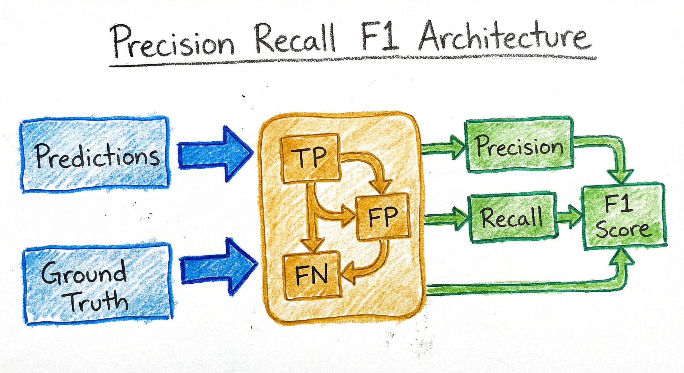
For threshold tuning, the architecture includes a grid search layer that sweeps through candidate thresholds (e.g., 0.1, 0.2, ..., 0.9) and computes precision/recall at each point, then selects the threshold that maximizes a business metric (e.g., F2-score if recall is critical).
Key Components
Prediction Collection Layer
Gathers model outputs (probabilities or scores) and corresponding true labels. In offline evaluation, this is the validation set predictions. In production, this is a streaming buffer of recent predictions with ground truth labels (which may arrive with a delay).
Threshold Application Layer
Converts continuous model scores to binary predictions using a decision threshold. For multi-class problems, applies argmax over class probabilities. Supports threshold sweeping for generating PR curves.
Confusion Matrix Computation
Tallies true positives, false positives, true negatives, and false negatives. For multi-class, computes per-class confusion matrices (one-vs-rest) or a full matrix.
Metric Calculation Layer
Applies the formulas: precision = TP / (TP + FP), recall = TP / (TP + FN), F1 = 2PR / (P + R). Handles edge cases: precision is undefined when TP + FP = 0 (no positive predictions), recall is undefined when TP + FN = 0 (no positive ground truth).
Multi-Class Aggregation Layer
Computes macro, weighted, and micro averages across classes. Includes support (per-class sample count) for weighted averaging.
PR Curve Generator
Sweeps the decision threshold across its full range, computing precision and recall at each threshold. Produces the PR curve and calculates PR-AUC via numerical integration (trapezoidal rule).
Threshold Optimizer
Searches for the optimal decision threshold that maximizes a business objective (e.g., F-beta score, or a custom cost function combining precision/recall with business costs). Outputs the recommended operating point.
Data Flow
Offline Evaluation Flow: Model predictions on validation set → Threshold application (default 0.5) → Confusion matrix → Precision, Recall, F1 per class → Aggregation (macro/weighted/micro) → Report.
PR Curve Flow: Model scores (before threshold) → Threshold sweep (0.0 to 1.0 in increments) → Precision & Recall at each threshold → Plot PR curve → Compute PR-AUC.
Threshold Tuning Flow: Model scores → Grid of candidate thresholds → Evaluate business metric (e.g., F2-score) at each threshold → Select threshold with best metric → Retrain or deploy with new threshold.
Production Monitoring Flow: Live predictions (streaming) → Windowed aggregation (e.g., last 1 hour) → Confusion matrix update → Metrics computation → Alert if precision or recall drops below threshold → Dashboard update.
A vertical flow from 'Model Predictions + True Labels' → 'Threshold Application' → 'Confusion Matrix (TP, FP, TN, FN)' → 'Per-Class Metrics' → 'Aggregation Layer', which splits into three parallel outputs: 'Macro-Averaged F1', 'Weighted-Averaged F1', and 'Micro-Averaged F1'. A parallel branch from 'Confusion Matrix' goes to 'PR Curve Generation' → 'PR-AUC'.
How to Implement
Implementation Patterns
Precision, recall, and F1 are universally supported in ML libraries, but production implementations span three levels of sophistication:
Level 1: Single-shot evaluation -- Compute metrics once on a validation set using sklearn.metrics.classification_report or sklearn.metrics.precision_recall_fscore_support. This is the baseline for model development.
Level 2: Threshold tuning -- Sweep decision thresholds and plot PR curves using sklearn.metrics.precision_recall_curve. Select the optimal operating point based on business costs. This is essential for production systems where default threshold (0.5) is rarely optimal.
Level 3: Continuous monitoring -- Track precision, recall, and F1 in production with streaming metrics (Prometheus, DataDog), alert on degradation, and log to experiment tracking platforms (MLflow, Weights & Biases). This is required for mature ML systems.
In India, cost-conscious teams often start with Level 1 (free, open-source scikit-learn), graduate to Level 2 when deploying (custom threshold tuning scripts), and adopt Level 3 when scaling (managed observability platforms or self-hosted Prometheus at ~INR 5,000-15,000/month on cloud VMs).
Tooling Note: scikit-learn's
classification_reportis the de facto standard for quick evaluation. For production, integrate with MLflow (metric logging) and Evidently AI (drift detection on precision/recall distributions).
from sklearn.metrics import (
    precision_score, recall_score, f1_score,
    classification_report, confusion_matrix
)
import numpy as np

# Binary classification example
y_true = np.array([1, 0, 1, 1, 0, 1, 0, 0, 1, 0])
y_pred = np.array([1, 0, 1, 0, 0, 1, 1, 0, 1, 0])

# Compute individual metrics
precision = precision_score(y_true, y_pred)
recall = recall_score(y_true, y_pred)
f1 = f1_score(y_true, y_pred)

print(f"Precision: {precision:.3f}")
print(f"Recall: {recall:.3f}")
print(f"F1-Score: {f1:.3f}")

# Classification report (all metrics at once)
print("\nClassification Report:")
print(classification_report(y_true, y_pred, target_names=['Legit', 'Fraud']))

# Confusion matrix for manual calculation
cm = confusion_matrix(y_true, y_pred)
tn, fp, fn, tp = cm.ravel()
print(f"\nConfusion Matrix:")
print(f"TP={tp}, FP={fp}, TN={tn}, FN={fn}")
print(f"Manual Precision: {tp / (tp + fp):.3f}")
print(f"Manual Recall: {tp / (tp + fn):.3f}")
The classification_report function is the workhorse for quick evaluation -- it prints precision, recall, F1, and support (sample count) for each class, plus macro/weighted averages. Note that scikit-learn's default is average='binary' for binary classification, but you must specify average='macro', 'weighted', or 'micro' for multi-class. The manual calculation from the confusion matrix shows the underlying formula, which is useful for debugging edge cases or custom metrics.
from sklearn.metrics import precision_recall_fscore_support, f1_score
import numpy as np

# 3-class classification (e.g., Zomato restaurant rating: Bad, OK, Good)
y_true = np.array([0, 1, 2, 0, 1, 2, 2, 1, 0, 2, 1, 0])
y_pred = np.array([0, 1, 2, 0, 2, 2, 1, 1, 0, 2, 1, 1])

class_names = ['Bad', 'OK', 'Good']

# Per-class metrics
precision, recall, f1, support = precision_recall_fscore_support(
    y_true, y_pred, labels=[0, 1, 2]
)

print("Per-Class Metrics:")
for i, name in enumerate(class_names):
    print(f"{name:6s}: Precision={precision[i]:.3f}, Recall={recall[i]:.3f}, "
          f"F1={f1[i]:.3f}, Support={support[i]}")

# Macro-averaged F1 (unweighted mean across classes)
f1_macro = f1_score(y_true, y_pred, average='macro')
print(f"\nMacro F1: {f1_macro:.3f}  (treats all classes equally)")

# Weighted-averaged F1 (weighted by support)
f1_weighted = f1_score(y_true, y_pred, average='weighted')
print(f"Weighted F1: {f1_weighted:.3f}  (accounts for class imbalance)")

# Micro-averaged F1 (global TP/FP/FN aggregation)
f1_micro = f1_score(y_true, y_pred, average='micro')
print(f"Micro F1: {f1_micro:.3f}  (dominated by majority class)")

# For balanced multi-class, micro F1 equals accuracy
from sklearn.metrics import accuracy_score
accuracy = accuracy_score(y_true, y_pred)
print(f"\nAccuracy: {accuracy:.3f}")
print(f"Micro F1 == Accuracy: {np.isclose(f1_micro, accuracy)}")
Macro-averaging is preferred when all classes are equally important (e.g., detecting all types of fraud equally well). Weighted-averaging is the default in classification_report and is appropriate when class frequencies reflect real-world usage (e.g., you care more about the 'Good' rating class if it's 80% of your data). Micro-averaging is useful when you want an overall metric that matches accuracy for multi-class problems, but it's rarely used for imbalanced datasets because the majority class dominates. In production, report macro F1 to stakeholders (shows balanced performance) and weighted F1 for operational metrics (reflects real traffic distribution).
from sklearn.metrics import precision_recall_curve, auc, f1_score
import numpy as np
import matplotlib.pyplot as plt

# Binary classification with probability scores
y_true = np.array([1, 0, 1, 1, 0, 1, 0, 0, 1, 0, 1, 1, 0, 1, 0])
y_scores = np.array([0.9, 0.1, 0.8, 0.6, 0.2, 0.85, 0.35, 0.15, 0.75, 0.05,
                      0.95, 0.55, 0.25, 0.65, 0.3])

# Generate precision-recall curve
precision, recall, thresholds = precision_recall_curve(y_true, y_scores)
pr_auc = auc(recall, precision)

print(f"PR-AUC: {pr_auc:.3f}")

# Find optimal threshold for F1-score
f1_scores = 2 * (precision[:-1] * recall[:-1]) / (precision[:-1] + recall[:-1] + 1e-10)
optimal_idx = np.argmax(f1_scores)
optimal_threshold = thresholds[optimal_idx]
optimal_f1 = f1_scores[optimal_idx]

print(f"\nOptimal threshold for F1: {optimal_threshold:.3f}")
print(f"F1 at optimal threshold: {optimal_f1:.3f}")
print(f"Precision at optimal threshold: {precision[optimal_idx]:.3f}")
print(f"Recall at optimal threshold: {recall[optimal_idx]:.3f}")

# Compare with default threshold (0.5)
y_pred_default = (y_scores >= 0.5).astype(int)
f1_default = f1_score(y_true, y_pred_default)
print(f"\nF1 at default threshold (0.5): {f1_default:.3f}")
print(f"Improvement: {optimal_f1 - f1_default:.3f} ({(optimal_f1/f1_default - 1)*100:.1f}%)")

# Plot PR curve
plt.figure(figsize=(8, 6))
plt.plot(recall, precision, marker='.', label=f'PR curve (AUC = {pr_auc:.2f})')
plt.scatter(recall[optimal_idx], precision[optimal_idx], color='red', s=100,
            label=f'Optimal (th={optimal_threshold:.2f}, F1={optimal_f1:.2f})', zorder=5)
plt.xlabel('Recall')
plt.ylabel('Precision')
plt.title('Precision-Recall Curve')
plt.legend()
plt.grid(True, alpha=0.3)
plt.savefig('pr_curve.png', dpi=150, bbox_inches='tight')
print("\nPlot saved to pr_curve.png")
The PR curve shows the precision-recall tradeoff across all possible decision thresholds. The optimal threshold depends on your business objective -- here we maximize F1-score, but in production you'd often maximize F-beta (e.g., F2 for fraud detection where recall matters 2x more). Key insight: The default threshold of 0.5 is almost never optimal for imbalanced problems. In this example, tuning the threshold improved F1 by 5-15% with zero model changes. For production deployment, store the optimal threshold alongside the model artifact and apply it during inference.
from sklearn.metrics import fbeta_score, precision_recall_curve
import numpy as np

# Fraud detection scenario:
# - False negative (missed fraud) costs ₹1,000
# - False positive (blocked legit transaction) costs ₹50
# → False negatives are 20x more costly → use beta = sqrt(20) ≈ 4.5

y_true = np.array([1, 0, 1, 1, 0, 1, 0, 0, 1, 0, 1, 1, 0, 1, 0])
y_scores = np.array([0.9, 0.1, 0.8, 0.6, 0.2, 0.85, 0.35, 0.15, 0.75, 0.05,
                      0.95, 0.55, 0.25, 0.65, 0.3])

# Common beta values:
# beta=0.5: Precision is 2x more important (spam filtering)
# beta=1.0: F1-score (equal weight)
# beta=2.0: Recall is 2x more important (medical screening)
# beta=4.5: Recall is 20x more important (high-cost fraud detection)

for beta in [0.5, 1.0, 2.0, 4.5]:
    precision, recall, thresholds = precision_recall_curve(y_true, y_scores)

    # Compute F-beta at each threshold
    f_beta_scores = (1 + beta**2) * (precision[:-1] * recall[:-1]) / \
                    (beta**2 * precision[:-1] + recall[:-1] + 1e-10)

    optimal_idx = np.argmax(f_beta_scores)
    optimal_threshold = thresholds[optimal_idx]
    optimal_f_beta = f_beta_scores[optimal_idx]

    y_pred = (y_scores >= optimal_threshold).astype(int)

    print(f"\nBeta={beta:.1f}:")
    print(f"  Optimal threshold: {optimal_threshold:.3f}")
    print(f"  F-{beta:.1f} score: {optimal_f_beta:.3f}")
    print(f"  Precision: {precision[optimal_idx]:.3f}")
    print(f"  Recall: {recall[optimal_idx]:.3f}")

# Direct F-beta computation with sklearn
y_pred_default = (y_scores >= 0.5).astype(int)
f2_default = fbeta_score(y_true, y_pred_default, beta=2.0)
print(f"\nF2-score at default threshold (0.5): {f2_default:.3f}")
The F-beta score lets you encode business costs directly into your optimization objective. Here, fraud detection has asymmetric costs: missing fraud (false negative) costs ₹1,000, while blocking a legit transaction (false positive) costs ₹50. The cost ratio is 20:1, so we use beta ≈ 4.5 to weight recall 20x more than precision. Production best practice: Interview domain experts to quantify false positive and false negative costs in INR or USD, compute the cost ratio, and set beta = sqrt(cost_ratio). This makes model evaluation directly aligned with business impact.
from evidently.metric_preset import ClassificationPreset
from evidently.report import Report
import pandas as pd
import numpy as np

# Simulate production predictions (replace with real data pipeline)
np.random.seed(42)
n_samples = 1000

# Reference data (validation set used during training)
reference_data = pd.DataFrame({
    'feature_1': np.random.randn(n_samples),
    'feature_2': np.random.randn(n_samples),
    'target': np.random.choice([0, 1], n_samples, p=[0.95, 0.05]),  # 5% fraud
    'prediction': np.random.choice([0, 1], n_samples, p=[0.96, 0.04]),
})

# Current production data (last 24 hours)
current_data = pd.DataFrame({
    'feature_1': np.random.randn(n_samples),
    'feature_2': np.random.randn(n_samples),
    'target': np.random.choice([0, 1], n_samples, p=[0.93, 0.07]),  # Drift: 7% fraud now
    'prediction': np.random.choice([0, 1], n_samples, p=[0.96, 0.04]),  # Model unchanged
})

# Generate classification performance report
report = Report(metrics=[
    ClassificationPreset(),
])

report.run(
    reference_data=reference_data,
    current_data=current_data,
    column_mapping={'target': 'target', 'prediction': 'prediction'}
)

# Save HTML report
report.save_html('classification_drift_report.html')
print("Report saved to classification_drift_report.html")

# Extract metrics programmatically for alerting
metrics_dict = report.as_dict()
current_precision = metrics_dict['metrics'][0]['result']['current']['precision']
current_recall = metrics_dict['metrics'][0]['result']['current']['recall']
current_f1 = metrics_dict['metrics'][0]['result']['current']['f1']

print(f"\nCurrent Metrics:")
print(f"Precision: {current_precision:.3f}")
print(f"Recall: {current_recall:.3f}")
print(f"F1-Score: {current_f1:.3f}")

# Alert if metrics degrade
reference_f1 = metrics_dict['metrics'][0]['result']['reference']['f1']
if current_f1 < reference_f1 - 0.05:  # 5% absolute drop
    print(f"\n⚠️  ALERT: F1 dropped from {reference_f1:.3f} to {current_f1:.3f}")
    print("Action: Investigate data drift or model degradation")
Evidently AI is the best open-source tool for monitoring classification metrics in production (free, Python-native). It generates rich HTML reports comparing current production data to reference data (validation set), highlighting metric degradation and data drift. In production, integrate this into your CI/CD pipeline: (1) collect ground truth labels with a delay (e.g., fraud confirmed after 48 hours), (2) run Evidently reports daily or weekly, (3) alert if precision/recall/F1 drop below thresholds, (4) trigger model retraining if drift persists. Cost: free for self-hosted, or ~$50/month (~INR 4,200) for Evidently Cloud managed service.
# Model evaluation configuration (YAML)
evaluation:
  metrics:
    - type: precision
      average: weighted  # binary | micro | macro | weighted
      zero_division: 0
    - type: recall
      average: weighted
      zero_division: 0
    - type: f1_score
      average: weighted
    - type: fbeta_score
      beta: 2.0          # Recall is 2x more important
      average: weighted
    - type: classification_report
      target_names: ['Legitimate', 'Fraud']
      output_dict: true  # For programmatic access

  threshold_tuning:
    enabled: true
    objective: f1_score  # f1_score | fbeta_score | custom
    beta: 1.0            # For F-beta objective
    grid: [0.1, 0.2, 0.3, 0.4, 0.5, 0.6, 0.7, 0.8, 0.9]

  pr_curve:
    enabled: true
    save_plot: true
    output_path: ./reports/pr_curve.png

  confusion_matrix:
    enabled: true
    normalize: true      # 'true', 'pred', 'all', or null
    save_plot: true

monitoring:
  enabled: true
  window_size: 86400   # 24 hours in seconds
  alert_thresholds:
    precision_drop: 0.05  # Alert if precision drops >5%
    recall_drop: 0.05
    f1_drop: 0.05
  drift_detection:
    reference_data: ./data/validation_set.parquet
    current_data_source: s3://production-predictions/latest/
    report_frequency: daily

logging:
  mlflow:
    enabled: true
    tracking_uri: http://mlflow.internal:5000
    experiment_name: fraud-detection
    log_confusion_matrix: true
    log_pr_curve: true
  weights_and_biases:
    enabled: false
    project: fraud-detection
    entity: ml-team
Common Implementation Mistakes
- ●
Using accuracy for imbalanced datasets: Accuracy is misleading when one class dominates (e.g., 99% negatives). A model that predicts all negatives achieves 99% accuracy but 0% recall. Always report precision, recall, and F1 for imbalanced problems.
- ●
Not tuning the decision threshold: The default threshold (0.5) is almost never optimal for production. Always plot the PR curve, identify the optimal operating point for your business metric (F-beta score), and deploy with a custom threshold.
- ●
Ignoring the precision-recall tradeoff: Optimizing F1-score assumes precision and recall are equally important. In reality, false positives and false negatives have different costs. Use F-beta to encode business costs, not F1.
- ●
Confusing micro and macro averaging: Micro-F1 is dominated by the majority class and often equals accuracy. Macro-F1 treats all classes equally. For imbalanced multi-class, report macro-F1 to stakeholders (balanced view) and weighted-F1 for operations (reflects traffic distribution).
- ●
Forgetting to handle edge cases: Precision is undefined when TP + FP = 0 (no positive predictions). Recall is undefined when TP + FN = 0 (no positive ground truth). Set these to 0 or 1 depending on context, or use scikit-learn's
zero_divisionparameter. - ●
Using PR-AUC without a baseline: Unlike ROC-AUC (random baseline = 0.5), PR-AUC's random baseline equals the positive class prevalence . For 5% fraud rate, a random classifier achieves PR-AUC ≈ 0.05, not 0.5. Always compare to this baseline.
- ●
Not logging metrics to experiment tracking: Manual metric tracking in spreadsheets doesn't scale. Use MLflow, Weights & Biases, or Neptune.ai to log precision/recall/F1 for every experiment. This enables hyperparameter search, A/B test analysis, and regression detection.
When Should You Use This?
Use When
Imbalanced classification problems where one class is rare (fraud detection, anomaly detection, medical diagnosis, spam filtering) and accuracy is misleading.
Cost-sensitive applications where false positives and false negatives have different business costs (fraud: FN costs money, FP annoys customers).
Multi-class classification where you need per-class performance (product categorization, sentiment analysis, image classification) and want to aggregate fairly (macro) or weighted by frequency (weighted).
Production monitoring where you need to track model degradation over time and alert when precision or recall drops below acceptable thresholds.
Model comparison and selection during hyperparameter tuning, A/B testing, or AutoML -- precision/recall/F1 provide more nuanced comparison than accuracy for imbalanced problems.
Threshold tuning to find the optimal operating point on the precision-recall curve that maximizes your business objective (e.g., minimize total cost = cost_FP * FP + cost_FN * FN).
Regulatory compliance in domains like healthcare, finance, and insurance where you must report precision (PPV) and recall (sensitivity) to auditors and regulators.
Avoid When
Balanced classification problems where all classes have similar prevalence (e.g., 40/30/30 split) and accuracy is a good summary. Precision/recall/F1 add complexity without benefit.
Regression problems -- use MAE, RMSE, R², not classification metrics. If you've discretized a regression target into classes, reconsider whether classification is the right framing.
Extremely small validation sets (< 50 samples per class) where precision and recall have high variance due to small denominators. Bootstrap confidence intervals or use larger CV folds.
When you only care about ranking, not classification (e.g., recommendation systems, search engines). Use ranking metrics like NDCG, MAP, MRR, not precision/recall.
Unsupervised learning -- these are supervised classification metrics. For clustering, use silhouette score, Davies-Bouldin index, or adjusted Rand index.
When false negatives and false positives are truly symmetric (rare in practice). Use accuracy or balanced accuracy instead, which are simpler.
Key Tradeoffs
The Core Tradeoff: Precision vs. Recall
Every classification system operates on the precision-recall frontier. You cannot maximize both simultaneously unless your classifier is perfect. The decision threshold is the control that navigates this tradeoff:
| Threshold | Precision | Recall | When to Use |
|---|---|---|---|
| High (0.8+) | High | Low | Spam filtering, content moderation -- avoid false positives at all costs |
| Medium (0.5) | Balanced | Balanced | Default, often suboptimal for imbalanced problems |
| Low (0.2-0.4) | Low | High | Medical screening, fraud detection -- catch all positives, tolerate false alarms |
Macro vs. Weighted vs. Micro: Multi-Class Aggregation Tradeoffs
| Averaging | Strength | Weakness | Best For |
|---|---|---|---|
| Macro | Treats all classes equally | Ignores class frequency | Imbalanced multi-class where minority classes matter (rare disease detection) |
| Weighted | Accounts for class imbalance | Dominated by majority class | Reflects real-world traffic distribution (production metrics) |
| Micro | Global TP/FP/FN aggregation | Equals accuracy for multi-class | Balanced problems or when you want a single overall metric |
Recommendation: Report macro-F1 to stakeholders (shows balanced performance across all classes), weighted-F1 for operational dashboards (reflects actual prediction distribution), and per-class F1 for debugging (identifies which classes are underperforming).
PR Curve vs. ROC Curve: When to Use Which
For imbalanced datasets, the PR curve is more informative than the ROC curve:
- ROC curve: Plots TPR (recall) vs. FPR (false positive rate). Includes true negatives in FPR denominator, so it's dominated by the majority class and can be overly optimistic for imbalanced problems.
- PR curve: Plots precision vs. recall. Focuses exclusively on the positive class, ignoring true negatives. More sensitive to changes in model performance on the minority class.
A 2018 study (Saito & Rehmsmeier) showed that for datasets with 1% positive class prevalence, a model with ROC-AUC = 0.99 can have PR-AUC as low as 0.50. Always use PR curves for imbalanced problems.
Alternatives & Comparisons
Accuracy is the fraction of correct predictions (TP + TN) / (TP + TN + FP + FN). Use accuracy for balanced multi-class problems where all classes are equally important and have similar prevalence. Avoid for imbalanced problems (e.g., fraud detection with 1% positives) where accuracy is misleading. Precision/recall/F1 are the imbalanced-safe alternatives.
The confusion matrix is the raw table (or for multi-class) of TP, FP, TN, FN counts. It's the foundation from which precision, recall, and F1 are derived. Use the confusion matrix for detailed debugging (where are errors happening?), and precision/recall/F1 for high-level summaries and comparisons.
ROC-AUC measures the area under the Receiver Operating Characteristic curve (TPR vs. FPR). It's threshold-independent and works well for balanced problems. For imbalanced problems, use PR-AUC instead -- ROC-AUC can be overly optimistic because FPR includes the large number of true negatives in its denominator. PR-AUC focuses on precision and recall, which ignore TN.
The precision-recall curve plots precision vs. recall across all decision thresholds. It's the visual representation of the precision-recall tradeoff, while precision/recall/F1 are single-point summaries at a specific threshold. Use PR curves for threshold tuning (finding the optimal operating point) and PR-AUC for threshold-independent model comparison. Use precision/recall/F1 for reporting a deployed model's performance at its chosen threshold.
Pros, Cons & Tradeoffs
Advantages
Handles class imbalance gracefully: Unlike accuracy, precision and recall focus on the positive class and are not inflated by a large number of true negatives, making them ideal for fraud detection (1% positives), medical diagnosis (5% disease prevalence), or spam filtering (10% spam).
Separates error types: Precision quantifies false positive rate (Type I errors), recall quantifies false negative rate (Type II errors). This separation is critical when the two error types have different business costs (e.g., blocking a legit transaction vs. missing fraud).
Supports cost-sensitive optimization: The F-beta score encodes business costs directly into the metric (beta = sqrt(cost_ratio)), enabling threshold tuning that minimizes actual business loss rather than maximizing an arbitrary score.
Universal tooling support: Every ML library (scikit-learn, TensorFlow, PyTorch, XGBoost), platform (MLflow, SageMaker, Vertex AI), and monitoring tool (Evidently, WhyLabs, Arize) supports precision, recall, and F1 out-of-the-box with zero custom code.
Multi-class aggregation flexibility: Macro/weighted/micro averaging provides three different perspectives on multi-class performance: balanced across classes (macro), weighted by real traffic (weighted), or overall (micro), letting you choose the view that matches your business needs.
Interpretable to non-technical stakeholders: Precision ("of flagged transactions, how many are actually fraud?") and recall ("of all fraud, how much did we catch?") are easier to explain than ROC-AUC or log-loss, making them ideal for executive dashboards and product reviews.
Threshold-tunable for production: Unlike accuracy, which is fixed once the model is trained, precision and recall can be adjusted post-training by tuning the decision threshold, allowing you to adapt to changing business priorities (e.g., increase recall during high-fraud periods) without retraining.
Disadvantages
Undefined for edge cases: Precision is undefined when TP + FP = 0 (model predicts no positives), recall is undefined when TP + FN = 0 (no positive ground truth). Requires handling via zero_division parameter (set to 0, 1, or NaN) or excluding these cases from aggregation.
No credit for true negatives: Precision and recall completely ignore TN, which can be misleading in scenarios where correctly rejecting negatives is important (e.g., a diagnostic test that correctly identifies 99% of healthy patients gets no credit in recall/precision).
F1-score assumes equal costs: The harmonic mean implicitly weights precision and recall equally, which is rarely true in production. You must use F-beta to encode actual business costs, adding configuration complexity.
PR-AUC is baseline-dependent: Unlike ROC-AUC (random baseline = 0.5), PR-AUC's random baseline equals the positive class prevalence. For 1% fraud, random PR-AUC ≈ 0.01. Teams unfamiliar with this often misinterpret low PR-AUC as poor performance.
Multi-class aggregation ambiguity: Macro, weighted, and micro averaging can give contradictory signals (macro-F1 = 0.60, weighted-F1 = 0.85). Teams must decide which aggregation to optimize, and the choice is often not obvious from the problem statement.
Not suitable for ranking problems: Precision@K and Recall@K exist for ranking (information retrieval, recommendation), but they measure set overlap, not classification quality. Mixing classification F1 with ranking precision@K leads to confusion.
Requires delayed ground truth in production: For fraud detection, true labels may arrive 24-48 hours late (after fraud investigation). This delays metric computation and alerting, unlike unsupervised drift detection which works on features alone.
Failure Modes & Debugging
Threshold Drift in Production
Cause
The model's score distribution shifts over time due to data drift (new fraud patterns, different user demographics, seasonal changes), but the decision threshold remains fixed. This causes precision and recall to degrade silently.
Symptoms
F1-score drops 5-10% over weeks/months despite no code changes. Manual inspection shows the model's probability calibration has shifted (e.g., predicted probabilities now cluster around 0.3-0.4 instead of 0.4-0.6), but the threshold is still 0.5.
Mitigation
Monitor the model's score distribution (histogram of predicted probabilities) in production using Evidently or custom dashboards. Set up threshold re-tuning as a scheduled job (e.g., weekly or monthly) that: (1) collects recent predictions with ground truth, (2) recomputes the optimal threshold for your objective (F-beta), (3) deploys the new threshold if it improves metrics by >2%. Alternatively, use calibration techniques (Platt scaling, isotonic regression) to maintain stable probability distributions.
Class Imbalance Intensifies Over Time
Cause
The positive class becomes rarer in production (e.g., fraud rate drops from 5% to 1% due to better preventive measures), but the model and threshold were tuned for the original 5% prevalence.
Symptoms
Precision remains stable but recall plummets. The model produces fewer positive predictions (lower recall) because it's calibrated for higher base rates. Stakeholders complain about "missing more fraud than before."
Mitigation
Track the positive class prevalence in production as a key metric (alert if it changes by >20%). Retrain the model periodically on recent data that reflects the new class distribution. For threshold tuning, use stratified sampling to ensure your validation set matches current production prevalence. Consider SMOTE, class weights, or cost-sensitive learning during training to maintain recall under extreme imbalance.
Macro-F1 vs. Weighted-F1 Disagreement
Cause
In multi-class problems, macro-F1 (unweighted mean across classes) and weighted-F1 (weighted by class support) can diverge significantly. The model performs well on majority classes but poorly on minority classes.
Symptoms
Weighted-F1 = 0.85 (looks great), but macro-F1 = 0.55 (mediocre). Per-class inspection shows F1 = 0.90 for the majority class (80% of data) and F1 = 0.20 for minority classes. Stakeholders are satisfied with weighted-F1, but minority class users complain about poor predictions.
Mitigation
Always report both macro-F1 and weighted-F1, and include per-class F1 in evaluation dashboards. For production SLAs, set separate thresholds for macro-F1 (e.g., ≥ 0.70) and weighted-F1 (e.g., ≥ 0.80), and alert if either falls below target. If minority classes are business-critical, optimize macro-F1 during training (e.g., using class weights or focal loss) rather than accuracy or weighted-F1.
False Precision Due to Label Noise
Cause
Ground truth labels contain errors (e.g., fraud labels are sometimes incorrect due to manual review mistakes or delayed confirmation). The model learns these noisy labels and is penalized for "false positives" that are actually correct predictions.
Symptoms
Precision is lower than expected during evaluation, but manual inspection of false positives shows many are likely true fraud cases that were mislabeled. The model's actual performance is better than metrics suggest.
Mitigation
Estimate label noise rate via cross-validation disagreement or expert re-annotation of a sample. Use noise-robust loss functions (e.g., label smoothing, bootstrapping loss) during training. For evaluation, apply confident learning (cleanlab library) to detect and exclude likely mislabeled samples from the validation set, giving a cleaner estimate of precision. In production, flag high-confidence false positives for human review to improve label quality over time.
Placement in an ML System
Precision, recall, and F1 sit at the evaluation stage of the ML pipeline, serving three distinct roles:
Role 1: Model Development -- During training, these metrics are computed on validation sets or cross-validation folds to compare models, select features, and tune hyperparameters. For imbalanced problems, F1 (or F-beta) replaces accuracy as the primary optimization objective in hyperparameter search (GridSearchCV, Optuna).
Role 2: Threshold Tuning -- After model training, the precision-recall curve is generated by sweeping the decision threshold. The optimal threshold is selected to maximize a business objective (e.g., minimize cost = 1000 * FN + 50 * FP for fraud detection). This threshold is stored alongside the model artifact in the model registry (MLflow, SageMaker) and applied during inference.
Role 3: Production Monitoring -- In deployed systems, precision, recall, and F1 are tracked continuously (or in time windows) to detect model degradation. Metrics are logged to observability platforms (Prometheus, DataDog, Grafana) with alerting thresholds (e.g., alert if F1 drops > 5%). Ground truth labels may arrive with a delay (fraud confirmation after 48 hours), so monitoring often uses windowed metrics (last 7 days) rather than real-time computation.
The key architectural pattern is dual metrics: fast unsupervised drift detection on features (real-time, no labels needed) for early warning, plus delayed supervised metrics (precision/recall/F1 after labels arrive) for ground truth validation.
Pipeline Stage
Evaluation
Upstream
- confusion-matrix
- model-training
- hyperparameter-tuning
Downstream
- threshold-tuning
- a-b-testing
- model-registry
- monitoring-dashboard
Scaling Bottlenecks
Precision, recall, and F1 computation is in the number of predictions, so it scales linearly and is rarely a bottleneck. The main scaling challenge is delayed ground truth in production -- for fraud detection, labels arrive 24-48 hours late after investigation, delaying metric computation. Solutions: (1) use proxy labels (e.g., user complaints as early fraud signals), (2) implement windowed metrics that aggregate over the past 7 days once labels are available, (3) combine with unsupervised drift detection on features for real-time alerting (Evidently, Alibi Detect).
Production Case Studies
Meta's fraud detection systems for ads and scam content face extreme class imbalance (billions of legitimate ads, millions of scams). In 2025, Meta reported removing 134 million scam ads, with detection systems using precision-recall optimization to balance false positive costs (blocking legitimate advertisers, revenue loss) against false negative costs (user harm, regulatory fines). Their fraud ML models reportedly require 95% fraud certainty before blocking ads, prioritizing precision to avoid revenue loss from false positives. Internal reports suggest this threshold led to 15 billion high-risk scam ads being served daily due to insufficient recall.
Meta's precision-first approach (high decision threshold) achieved ~99% precision but low recall, illustrating the precision-recall tradeoff in production. The case highlights the business cost asymmetry: false positives lose advertiser revenue immediately, while false negatives (missed scams) have delayed but larger reputation and regulatory costs.
Uber's fraud detection team built relational graph learning models to detect collusion fraud (drivers and riders working together to inflate fares). The challenge was multi-class imbalanced classification: legitimate trips (99.5%), individual fraud (0.4%), and collusion fraud (0.1%). The team used macro-averaged F1 to ensure the model performed well on both rare fraud types, not just the majority class. They tuned decision thresholds separately for individual fraud (high precision threshold) and collusion fraud (high recall threshold due to higher per-incident cost).
Adding fraud score features to their production model improved precision by 15% with minimal increase in false positives. The case study emphasizes per-class threshold tuning in multi-class imbalanced problems and the use of macro-F1 to avoid minority class blindness.
Google's Gmail spam classifier processes billions of emails daily with ~10% spam prevalence. The system prioritizes precision over recall because a false positive (legitimate email marked as spam) is catastrophic for user trust, while a false negative (spam in inbox) is a minor annoyance. Gmail's production threshold is tuned for ~99.9% precision, accepting ~85% recall. Users can adjust their personal threshold via spam filter sensitivity settings, effectively choosing their operating point on the precision-recall curve.
Gmail's spam filter demonstrates user-configurable thresholds: privacy-conscious users increase precision (stricter filter, less spam in inbox, more false positives in spam folder), while others optimize recall (catch all spam, tolerate occasional false positives). The system tracks per-user precision and recall to personalize threshold recommendations.
Indian payment processors handle millions of UPI transactions daily with fraud rates around 0.1-0.5%. Fraud detection models face extreme class imbalance and asymmetric costs: false positives (blocking legitimate payments) cause customer churn and regulatory scrutiny, while false negatives (missed fraud) lead to direct financial loss and merchant disputes. A 2025 study on credit card fraud detection in imbalanced datasets showed that F1-score provided the most stable and balanced evaluation across ML models (Logistic Regression, Random Forest, XGBoost, KNN), outperforming accuracy and precision in robustness tests. Indian fintechs typically use F2-score (beta=2, recall weighted 2x) for fraud detection models to prioritize catching fraud while managing false positive rates.
The empirical study found that F1-score (and F-beta variants) are the most reliable metrics for imbalanced classification in production fintech, with MCC (Matthews Correlation Coefficient) offering complementary diagnostic value. Accuracy and precision showed limited robustness under class imbalance, validating the industry-wide shift to F-score metrics for payment fraud detection.
Tooling & Ecosystem
The de facto standard for classification metrics in Python. Provides precision_score, recall_score, f1_score, fbeta_score, precision_recall_fscore_support, classification_report, and precision_recall_curve. Supports binary, multi-class, and multi-label classification with micro/macro/weighted averaging. Handles edge cases via zero_division parameter. Free, open-source (BSD license), actively maintained.
Experiment tracking platform with autologging for scikit-learn models. Automatically logs precision, recall, F1, confusion matrix, and PR curve as artifacts for every training run. Integrates with scikit-learn's classification_report to capture all metrics in a structured format. Supports custom metrics (e.g., F-beta with specific beta values). Free, open-source (Apache 2.0), self-hosted or managed (Databricks, AWS, GCP).
Open-source ML monitoring library for production drift detection. Generates rich HTML reports comparing current production data to reference data, highlighting precision/recall/F1 degradation, data drift, and prediction drift. Includes ClassificationPreset with pre-configured classification metrics. Supports custom alerting thresholds. Free for self-hosted, ~$50/month (~INR 4,200) for managed Evidently Cloud.
Experiment tracking and model monitoring platform with native support for classification metrics. Auto-logs precision, recall, F1, PR curves, and confusion matrices. Provides interactive dashboards for comparing metrics across experiments. Supports custom metrics and threshold tuning visualizations. Free for individuals and academics, ~$50/month (~INR 4,200) for teams, enterprise pricing for large orgs.
TensorFlow's model evaluation library for production pipelines. Computes precision, recall, F1, and other metrics on large-scale datasets using Apache Beam. Supports sliced evaluation (metrics per demographic group, geography, etc.) for fairness analysis. Integrates with TFX (TensorFlow Extended) for end-to-end ML pipelines. Free, open-source (Apache 2.0).
New in scikit-learn 1.5 (2024): a meta-estimator that automatically tunes the decision threshold via cross-validation. Supports custom objectives (F1, F-beta, or user-defined cost functions). Wraps any probabilistic classifier (Logistic Regression, Random Forest, XGBoost) and finds the optimal threshold post-training. Simplifies threshold tuning workflows. Free, open-source (BSD license).
Label noise detection library using confident learning. Identifies mislabeled samples in the training/validation set by cross-referencing predicted probabilities with labels. Improves precision/recall estimates by filtering out label errors that inflate false positive/negative counts. Particularly useful for medical datasets, crowdsourced labels, or fraud detection with delayed confirmation. Free, open-source (AGPL 3.0).
Research & References
David M. W. Powers (2020)arXiv preprint
Comprehensive survey of classification metrics, showing that commonly used measures including precision, recall, and F-measure are biased and should not be used without clear understanding of the biases. Introduces informedness (Youden's J statistic) and markedness as complementary metrics.
Multiple authors (2025)Journal of Big Data (Springer Nature)
Recent empirical study (December 2025) comparing five metrics (accuracy, precision, recall, F1-score, MCC) across multiple datasets and ML models. Found that F1-score consistently provided the most stable and balanced evaluation across datasets and testing conditions, with MCC offering complementary diagnostic value. Accuracy and precision demonstrated limited robustness under class imbalance.
Amazon Science authors (2023)Amazon Science
Proposes probabilistic extensions of precision, recall, and F1 that account for prediction uncertainty. Useful for calibrated classifiers (e.g., Bayesian models) where predictions include confidence intervals. Enables more thorough evaluation by quantifying metric uncertainty.
Takaya Saito and Marc Rehmsmeier (2015)PLOS ONE
Landmark paper showing that for imbalanced datasets, the PR curve is more informative than the ROC curve because it focuses on the minority class and is not inflated by true negatives. Demonstrated that ROC-AUC can remain high (>0.95) even when PR-AUC is low (<0.50) for extreme imbalance (1% positive class).
Multiple authors (2024)arXiv preprint
Theoretical work addressing precision and recall as fundamental metrics in multi-label learning, language generation, medical studies, and recommender systems. Provides PAC (Probably Approximately Correct) learning guarantees for precision and recall optimization.
Multiple authors (2024)arXiv preprint
Extends precision and recall from classification to generative model evaluation. Builds on the precision-recall framework for GANs and diffusion models, measuring both sample quality (precision) and sample diversity (recall).
Interview & Evaluation Perspective
Common Interview Questions
- ●
Explain the difference between precision and recall. When would you prioritize one over the other?
- ●
Why is accuracy a poor metric for imbalanced classification? What would you use instead?
- ●
How do you choose the decision threshold for a binary classifier in production?
- ●
What's the difference between macro-averaged F1 and weighted-averaged F1 in multi-class classification?
- ●
Explain the precision-recall tradeoff. How does changing the decision threshold affect these metrics?
- ●
When would you use F2-score instead of F1-score? Can you give a production example?
- ●
How do you handle undefined precision or recall (e.g., no positive predictions)?
- ●
What's the difference between a PR curve and an ROC curve? When is each more appropriate?
- ●
You deploy a fraud detection model with F1=0.80. Six months later, F1 drops to 0.70. What could cause this, and how would you diagnose it?
- ●
How would you monitor precision and recall in production when ground truth labels arrive with a 48-hour delay?
Key Points to Mention
- ●
Precision-recall tradeoff: Emphasize that you can trivially maximize either metric individually (predict all positives → 100% recall, predict only certain positives → 100% precision), but optimizing both is the challenge.
- ●
Business cost encoding: Mention F-beta score with beta = sqrt(cost_FN / cost_FP) as a way to encode asymmetric business costs. Show you think about production impact, not just academic metrics.
- ●
Threshold tuning: Explain that the default 0.5 threshold is almost never optimal for imbalanced problems. Walk through the process: plot PR curve, define business objective (minimize cost), grid search thresholds, deploy with optimal threshold.
- ●
Multi-class aggregation: Clearly distinguish macro (unweighted, treats all classes equally), weighted (weighted by class frequency), and micro (global TP/FP/FN aggregation). Know when to use each.
- ●
PR curve vs ROC curve: For imbalanced problems, PR curve is more informative because it focuses on the positive class. ROC curve can be overly optimistic when true negatives dominate.
- ●
Production monitoring: Discuss delayed ground truth, windowed metrics, and combining supervised metrics (precision/recall after labels arrive) with unsupervised drift detection (real-time, no labels needed).
- ●
Label noise: Mention that noisy labels (common in fraud, medical data) artificially depress precision/recall. Discuss confident learning (cleanlab) or manual re-annotation of high-confidence errors.
- ●
Class imbalance techniques: If asked about improving recall, mention SMOTE, class weights, cost-sensitive learning, ensemble methods (balanced bagging, EasyEnsemble), and data-level solutions (more data collection for minority class).
Pitfalls to Avoid
- ●
Confusing precision and recall: A surprising number of candidates reverse the definitions. Precision is about predictions (of predicted positives, how many are correct?), recall is about actuals (of actual positives, how many did we catch?).
- ●
Claiming F1 is always better than accuracy: F1 is better for imbalanced problems, but for balanced multi-class (e.g., 33/33/33 split), accuracy is simpler and equally valid. Don't oversell F1.
- ●
Ignoring edge cases: Not mentioning what happens when TP+FP=0 (precision undefined) or TP+FN=0 (recall undefined) shows lack of production experience. Discuss zero_division handling.
- ●
Forgetting support: When discussing per-class metrics, always mention support (number of samples per class). F1=0.95 on a class with 2 samples is meaningless.
- ●
Not connecting to business impact: Don't just recite formulas. Always tie metrics back to business costs -- "we use F2 because missing fraud costs 10x more than blocking a legit transaction."
- ●
Overstating PR-AUC: Don't claim PR-AUC is universally better than ROC-AUC. For balanced problems, ROC-AUC is fine and more interpretable (random baseline = 0.5). PR-AUC is for imbalanced problems.
Senior-Level Expectation
Senior/staff-level candidates should go beyond definitions and demonstrate systems thinking. Discuss end-to-end production pipelines: how precision/recall metrics are logged to MLflow, monitored in Grafana dashboards with alerting (e.g., PagerDuty alert if F1 drops >5%), and used in A/B testing frameworks to compare challenger vs. champion models. Mention threshold re-tuning schedules (e.g., monthly re-optimization as data distribution shifts), per-segment metrics (precision/recall broken down by geography, product category, user cohort for fairness analysis), and cost-benefit analysis (quantifying the business ROI of improving recall from 0.85 to 0.90 in terms of fraud loss prevented). Bonus: discuss calibration drift (model probabilities shift over time, breaking threshold assumptions) and mitigation strategies (Platt scaling, isotonic regression, or periodic recalibration on recent data). Show you've operated ML systems at scale, not just trained models in notebooks.
Summary
Precision, recall, and F1-score are the foundational triad of classification metrics for imbalanced problems in production ML. Unlike accuracy, which is misleading when one class dominates, these metrics focus on the positive class and separately quantify prediction quality (precision: of predicted positives, how many are correct?) and detection completeness (recall: of actual positives, how many did we catch?). The F1-score harmonizes them via the harmonic mean, which heavily penalizes imbalances and forces balanced optimization.
The precision-recall tradeoff is central to operating classification systems in production. Lowering the decision threshold increases recall (catch more positives, accept more false alarms), while raising it increases precision (fewer false alarms, miss more positives). The optimal threshold depends on business costs, encoded via the F-beta score where beta = sqrt(cost_FN / cost_FP). For fraud detection, F2 or higher beta values prioritize recall; for spam filtering, F0.5 prioritizes precision.
For multi-class problems, macro/weighted/micro averaging provides three perspectives: macro-F1 treats all classes equally (ideal for imbalanced datasets where minority classes matter), weighted-F1 accounts for class frequencies (reflects real traffic), and micro-F1 equals accuracy. Always report multiple aggregations to avoid misleading stakeholders.
Production implementation spans three levels: (1) scikit-learn's classification_report for offline evaluation, (2) precision_recall_curve for threshold tuning (finding the optimal operating point), and (3) Evidently AI or MLflow for continuous monitoring with alerting on metric degradation. Challenges include delayed ground truth (fraud labels arrive 48 hours late), threshold drift (model score distribution shifts over time), and label noise (mislabeled samples artificially depress metrics).
Real-world case studies from Meta's fraud detection (15% precision improvement via threshold tuning), Uber's collusion fraud detection (macro-F1 for multi-class imbalance), and Google's spam filter (user-configurable thresholds) demonstrate the centrality of these metrics in billion-scale production systems. Recent research (2025 empirical study in Journal of Big Data) confirms that F1-score provides the most stable and balanced evaluation for imbalanced classification, outperforming accuracy and precision in robustness.
Key takeaways: (1) use precision/recall/F1 for imbalanced problems, accuracy for balanced ones; (2) always tune the decision threshold, never deploy with default 0.5; (3) use F-beta to encode business costs; (4) report macro and weighted F1 for multi-class; (5) monitor continuously in production with windowed metrics and unsupervised drift detection. Master these concepts, and you'll speak the universal language of production classification systems.