Statistical Significance in Machine Learning
Here is the uncomfortable truth about deploying machine learning models: without rigorous statistical significance testing, you are essentially making multi-crore decisions based on vibes. You ran an A/B test, Model B lifted CTR by 0.3%, and now you want to ship it to 100 million users. But is that 0.3% real, or just noise from a Tuesday traffic spike?
Statistical significance is the mathematical framework that separates signal from noise in experiment results. It quantifies the probability that an observed difference between control and treatment groups is genuine rather than a product of random variation. In production ML systems, this translates directly to whether you should ship that new recommendation model, keep the old fraud detector, or extend the experiment another week.
The concept is deceptively simple on the surface -- compute a p-value, check if it is below 0.05, ship or don't ship. But real-world ML experimentation is vastly more complex. You are dealing with multiple simultaneous experiments, non-normal metric distributions, sequential peeking at results, variance from network effects, and the ever-present tension between statistical significance (is the effect real?) and practical significance (is the effect big enough to matter?).
Companies like Flipkart, Swiggy, Google, Netflix, and Microsoft run thousands of A/B tests annually. Every single one depends on getting statistical significance right. Get it wrong in one direction and you ship degraded experiences to millions of users. Get it wrong in the other direction and you kill promising innovations that never get a fair chance. This guide covers everything you need -- from foundational theory through production-grade implementation -- to make that call with confidence.
Concept Snapshot
- What It Is
- A quantitative determination of whether an observed experimental effect (e.g., a lift in conversion rate or reduction in latency from a new ML model) is unlikely to have occurred by chance alone, typically expressed through p-values, confidence intervals, and hypothesis test statistics.
- Category
- Evaluation
- Complexity
- Intermediate
- Inputs / Outputs
- Inputs: experiment data (control metrics, treatment metrics, sample sizes, significance level alpha, test type). Outputs: p-value, test statistic, confidence interval, statistical power, and a significance decision (reject or fail to reject the null hypothesis).
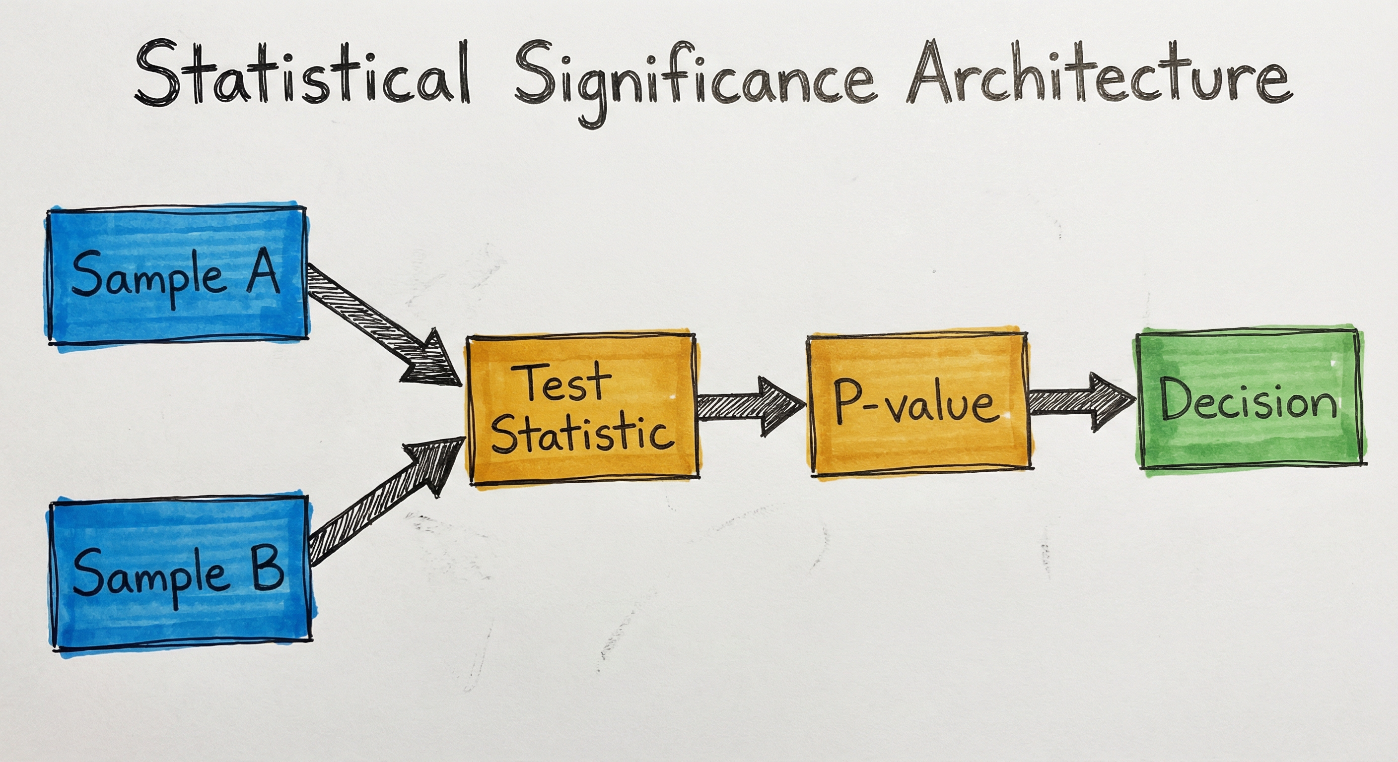
- System Placement
- Sits after the A/B test runner and before deployment decisions. In the ML pipeline, it operates during the evaluation and experimentation phase, receiving experiment data and producing go/no-go signals for model rollout.
- Also Known As
- Hypothesis Testing, Significance Testing, Statistical Hypothesis Test, Null Hypothesis Significance Testing (NHST), P-value Testing
- Typical Users
- Data Scientists, ML Engineers, Experimentation Platform Engineers, Product Managers, Growth Analysts, Biostatisticians
- Prerequisites
- Probability distributions (Normal, t, chi-squared), Central Limit Theorem, Sampling and sample size concepts, Basic A/B testing concepts, Descriptive statistics (mean, variance, standard deviation)
- Key Terms
- p-valueconfidence intervalnull hypothesis (H0)alternative hypothesis (H1)Type I error (false positive)Type II error (false negative)statistical powereffect sizesignificance level (alpha)t-testchi-squared testz-testBonferroni correctionfalse discovery rate (FDR)sequential testing
Why This Concept Exists
The Randomness Problem in ML Experiments
Every time you run an A/B test comparing two ML models, the results are contaminated by random variation. Users behave differently on Tuesdays than Thursdays. Weekend traffic on Swiggy looks nothing like Monday lunch traffic. A viral tweet can spike engagement for one variant by pure coincidence. Even with identical models, you would get different metric values each time you re-ran the experiment simply because different users ended up in each group.
Without statistical significance testing, you have no principled way to separate genuine model improvements from this background noise. You are essentially reading tea leaves -- seeing patterns in randomness and making costly infrastructure decisions based on them.
The Cost of Getting It Wrong
The consequences of incorrect significance decisions are asymmetric and severe. A false positive (Type I error) means you ship a model that is actually no better -- or worse -- than the current one. At scale, this degrades user experience for millions. Flipkart once reported that even a 0.1% degradation in search relevance translates to crores in lost GMV annually. A false negative (Type II error) means you kill a genuinely better model, leaving revenue on the table and demoralising the team that built it.
In high-stakes domains like healthcare ML (think Practo's diagnostic models) or financial fraud detection (Razorpay's payment risk scoring), the consequences multiply. A false positive could mean deploying a model that misses fraudulent transactions or misdiagnoses patients.
Historical Evolution
The intellectual foundations trace back to Ronald Fisher's work in the 1920s, who introduced the p-value as a measure of evidence against a null hypothesis while studying agricultural experiments at Rothamsted. Jerzy Neyman and Egon Pearson then formalised the framework with Type I errors, Type II errors, and statistical power in the 1930s, creating what we now call the Neyman-Pearson hypothesis testing framework.
For decades, these methods lived primarily in clinical trials and social science research. The internet era changed everything. When Ronny Kohavi brought rigorous A/B testing to Microsoft in the early 2000s and later published his seminal work on online controlled experiments, statistical significance testing became a core competency for every tech company. Today, platforms like Google, Netflix, Booking.com, and LinkedIn run thousands of simultaneous experiments, and the statistical machinery behind each decision has grown correspondingly sophisticated.
The Modern Challenge
Classical significance testing assumed a single experiment, tested once, with a pre-determined sample size. Modern ML experimentation violates every one of those assumptions. You peek at results continuously, run dozens of experiments on overlapping user populations, test multiple metrics simultaneously, and deal with metrics that are anything but normally distributed (revenue per user, for instance, follows a heavy-tailed distribution). This has driven innovation in sequential testing, multiple testing corrections, variance reduction techniques, and Bayesian alternatives -- all topics we will cover in depth.
Key Insight: Statistical significance testing exists because human intuition is catastrophically bad at distinguishing signal from noise in data. It provides a disciplined, reproducible framework for making decisions under uncertainty -- which is exactly what deploying ML models requires.
Core Intuition & Mental Model
The Courtroom Analogy
Think of statistical significance testing like a criminal trial. The null hypothesis (H0) is the presumption of innocence -- the claim that there is no real difference between your control and treatment models. The alternative hypothesis (H1) is the accusation -- that the treatment model genuinely performs differently.
Your experiment data is the evidence. The p-value is like a measure of how compelling that evidence is. Specifically, it answers: "If the defendant were truly innocent (H0 is true), what is the probability of seeing evidence this extreme or more extreme?" A tiny p-value means the evidence is highly unlikely under innocence, so you "convict" (reject H0) and conclude the treatment effect is real.
The significance level alpha (typically 0.05) is your conviction threshold -- how much evidence you demand before rejecting innocence. A Type I error is convicting an innocent person (false positive). A Type II error is acquitting a guilty person (false negative). Statistical power is the probability you successfully convict someone who is actually guilty.
Just as a "not guilty" verdict does not mean the defendant is innocent -- it means there was insufficient evidence -- failing to reject H0 does not mean the models are identical. It means your experiment did not produce enough evidence to conclude otherwise.
The Signal-to-Noise Ratio Mental Model
Here is an even more practical way to think about it. Imagine you are trying to hear someone whisper (the treatment effect) in a noisy room (random variation in user behaviour). Statistical significance is essentially asking: "Is this whisper loud enough relative to the background noise that I can be confident someone is actually speaking?"
Three things determine whether you can hear the whisper:
- How loud the whisper is (effect size) -- a 5% lift in conversion is easier to detect than a 0.1% lift.
- How noisy the room is (variance in your metric) -- revenue per user is noisier than click-through rate, so you need more data.
- How long you listen (sample size) -- more users in the experiment means the noise averages out, making even quiet whispers detectable.
Statistical significance formalises this intuition into mathematics: the test statistic is literally the observed effect divided by an estimate of the noise (the standard error). When this ratio exceeds a threshold, you declare significance.
Why 0.05?
Fisher originally described p < 0.05 as "convenient" -- a pragmatic threshold, not a law of nature. It means you accept a 5% chance of a false positive. For most ML experiments at companies like Zerodha or PhonePe, this is a reasonable tradeoff. But there is nothing sacred about it. In particle physics, the standard is 5 sigma (p < 0.0000003). In early-stage product experiments, some teams accept p < 0.10. The right threshold depends on the cost of being wrong.
Practical Insight: In ML systems, statistical significance answers "is this effect real?" but not "is this effect useful?" A recommendation model that lifts CTR by 0.001% might be statistically significant with 100 million users, but deploying it adds complexity for negligible business impact. Always pair statistical significance with practical significance -- the minimum effect size worth shipping.
Technical Foundations
Hypothesis Testing Framework
Given two populations (control and treatment ) with respective parameters and (e.g., mean conversion rates), we test:
Or for one-sided tests:
Test Statistics
Two-Sample Z-Test (large samples, known or estimated variance):
For proportions and with sample sizes and :
where is the pooled proportion.
Two-Sample T-Test (Welch's, unequal variances):
For means and with sample variances and :
Degrees of freedom (Welch-Satterthwaite):
Chi-Squared Test (categorical outcomes):
where are observed frequencies and are expected frequencies under , with degrees of freedom.
P-Value
The p-value is the probability of observing a test statistic as extreme as or more extreme than the computed value, assuming is true:
For a two-sided z-test: , where is the standard normal CDF.
Confidence Interval
A confidence interval for the difference in means:
where .
If this interval excludes zero, the result is significant at level .
Statistical Power and Sample Size
Power is the probability of correctly rejecting when a true effect of size exists:
For a two-sided z-test with equal group sizes:
where is the variance of the metric and is the minimum detectable effect (MDE).
Multiple Testing Correction
Bonferroni Correction: For simultaneous tests, use for each individual test. Controls the family-wise error rate (FWER).
Benjamini-Hochberg (BH) Procedure: For controlling the False Discovery Rate (FDR). Sort p-values and reject all where:
FDR is less conservative than FWER and better suited for exploratory analysis with many metrics.
Sequential Testing
In classical fixed-horizon testing, you set upfront and only analyse once. Sequential testing frameworks (e.g., group sequential methods, always-valid p-values) allow continuous monitoring with controlled Type I error:
The O'Brien-Fleming spending function allocates very little alpha to early looks, concentrating power at the final analysis:
Note: All these formulations assume independence of observations across users. Violations (e.g., network effects, shared households) require cluster-robust standard errors or specialised interference models.
Internal Architecture
A statistical significance testing system in production is far more than a single function call. It encompasses data collection, metric computation, variance estimation, test execution, multiple-testing correction, and decision reporting. The architecture must handle concurrent experiments, guard against peeking bias, and produce interpretable outputs for both technical and non-technical stakeholders.
The system operates in a feedback loop: experiments run continuously, metrics flow into the aggregator, significance is evaluated (often daily), and decisions are surfaced via dashboards. Sequential monitoring ensures that continuous peeking does not inflate the false positive rate, while multiple testing correction handles the reality that most experiments track 5-20 metrics simultaneously.
Key Components
Metric Aggregator
Collects raw event data from the experiment and computes per-variant summary statistics: sample sizes, means, variances, proportions, and quantiles. Handles metric definitions (count, ratio, revenue), applies pre-experiment filters (e.g., bot removal), and computes variance estimates using delta method for ratio metrics.
Test Engine (Z/T/Chi-squared)
Executes the appropriate hypothesis test based on metric type. For binary outcomes (click/no-click), uses a two-proportion z-test. For continuous metrics (revenue, latency), uses Welch's t-test. For categorical outcomes (multi-class preferences), uses chi-squared. Each engine returns a test statistic, p-value, and confidence interval.
Bootstrap Engine
Provides non-parametric significance testing for metrics that violate normality assumptions (e.g., heavy-tailed revenue distributions). Resamples the data with replacement times (typically 10,000), computes the test statistic for each resample, and builds an empirical null distribution. Particularly important for quantile metrics (p50 latency, p99 latency).
Multiple Testing Corrector
Adjusts p-values when multiple metrics or variants are tested simultaneously. Implements Bonferroni, Holm-Bonferroni, and Benjamini-Hochberg (FDR) corrections. Receives raw p-values from the test engine and returns adjusted p-values that control the appropriate error rate.
Sequential Monitor
Enables continuous experiment monitoring without inflating Type I error. Implements group sequential designs (O'Brien-Fleming, Pocock boundaries), always-valid p-values (based on confidence sequences), or mixture sequential probability ratio tests (mSPRT). Tracks cumulative alpha spending and gates early stopping decisions.
Power Calculator
Pre-experiment tool that determines required sample size given desired power (typically 80%), significance level (alpha = 0.05), baseline metric value, minimum detectable effect (MDE), and metric variance. Also performs post-hoc power analysis to interpret inconclusive results.
Decision Reporter
Generates human-readable reports combining statistical results with practical significance assessment. Flags cases where results are statistically significant but practically insignificant (tiny effect size) or vice versa. Outputs confidence intervals, relative lifts, and risk assessments for product teams.
Data Flow
Raw experiment events (impressions, clicks, conversions, revenue) flow from the A/B test runner into the experiment data store, partitioned by variant. The metric aggregator pulls this data and computes summary statistics per variant per metric. These summaries feed into the appropriate test engine based on metric type. Raw p-values from the test engine pass through multiple testing correction, then into the sequential monitor which compares against spending boundaries. Final results (adjusted p-values, confidence intervals, power estimates, practical significance flags) flow to the decision reporter, which produces dashboards and alerts for experiment owners.
The architecture diagram shows a flow starting from the A/B Test Runner feeding into an Experiment Data Store. Data flows to a Metric Aggregator, which routes to different test engines (Z-Test, T-Test/Welch's, Chi-Squared, Bootstrap) based on metric type. All engines feed into a Multiple Testing Correction module, then to a Sequential Monitor. The monitor branches to a Ship Decision if significant, an Inconclusive Report if maximum duration is reached, or loops back to continue the experiment.
How to Implement
Implementing statistical significance testing in production requires balancing mathematical rigour with engineering pragmatism. At its simplest, you can call scipy.stats.ttest_ind and check the p-value. At production scale, you need variance reduction (CUPED), sequential testing boundaries, bootstrap engines for non-normal metrics, and automated guardrail checks.
The implementation below progresses from foundational tests through production-grade patterns. Each example is complete and runnable with scipy, numpy, and statsmodels -- all standard in any ML environment. We also cover the often-overlooked practical significance check that separates junior from senior practitioners.
import numpy as np
from scipy import stats

def two_proportion_z_test(
    conversions_control: int,
    total_control: int,
    conversions_treatment: int,
    total_treatment: int,
    alpha: float = 0.05,
    one_sided: bool = False
) -> dict:
    """
    Two-proportion z-test for A/B tests on binary metrics
    (e.g., click-through rate, conversion rate).

    Returns p-value, z-statistic, confidence interval, and decision.
    """
    p_c = conversions_control / total_control
    p_t = conversions_treatment / total_treatment

    # Pooled proportion under H0
    p_pool = (conversions_control + conversions_treatment) / (
        total_control + total_treatment
    )

    # Standard error under H0
    se = np.sqrt(p_pool * (1 - p_pool) * (1/total_control + 1/total_treatment))

    # Z-statistic
    z_stat = (p_t - p_c) / se

    # P-value
    if one_sided:
        p_value = 1 - stats.norm.cdf(z_stat)
    else:
        p_value = 2 * (1 - stats.norm.cdf(abs(z_stat)))

    # Confidence interval for the difference (not pooled SE)
    se_diff = np.sqrt(p_t * (1 - p_t) / total_treatment +
                       p_c * (1 - p_c) / total_control)
    z_crit = stats.norm.ppf(1 - alpha / 2)
    ci_lower = (p_t - p_c) - z_crit * se_diff
    ci_upper = (p_t - p_c) + z_crit * se_diff

    return {
        "control_rate": p_c,
        "treatment_rate": p_t,
        "absolute_lift": p_t - p_c,
        "relative_lift_pct": ((p_t - p_c) / p_c) * 100 if p_c > 0 else float('inf'),
        "z_statistic": z_stat,
        "p_value": p_value,
        "confidence_interval": (ci_lower, ci_upper),
        "significant": p_value < alpha,
        "alpha": alpha,
    }


# Example: Flipkart search relevance A/B test
result = two_proportion_z_test(
    conversions_control=4820,
    total_control=50000,
    conversions_treatment=5140,
    total_treatment=50000,
    alpha=0.05
)

print(f"Control CVR: {result['control_rate']:.4f}")
print(f"Treatment CVR: {result['treatment_rate']:.4f}")
print(f"Relative lift: {result['relative_lift_pct']:.2f}%")
print(f"P-value: {result['p_value']:.4f}")
print(f"95% CI: ({result['confidence_interval'][0]:.4f}, {result['confidence_interval'][1]:.4f})")
print(f"Significant: {result['significant']}")
This is the workhorse test for binary A/B test metrics like conversion rate, click-through rate, or sign-up rate. It uses the pooled proportion under the null hypothesis to compute the standard error for the z-statistic, then computes the confidence interval using the unpooled standard error (which is appropriate for the CI since it does not assume H0). The function returns both absolute and relative lifts alongside the statistical verdict. In the Flipkart example, a lift from 9.64% to 10.28% CTR across 100K users is tested.
import numpy as np
from scipy import stats

def welch_t_test(
    control_data: np.ndarray,
    treatment_data: np.ndarray,
    alpha: float = 0.05,
    one_sided: bool = False
) -> dict:
    """
    Welch's t-test for continuous metrics (e.g., revenue per user,
    latency). Does not assume equal variances.
    """
    n_c, n_t = len(control_data), len(treatment_data)
    mean_c, mean_t = np.mean(control_data), np.mean(treatment_data)
    var_c, var_t = np.var(control_data, ddof=1), np.var(treatment_data, ddof=1)

    # Standard error of the difference
    se = np.sqrt(var_c / n_c + var_t / n_t)

    # T-statistic
    t_stat = (mean_t - mean_c) / se

    # Welch-Satterthwaite degrees of freedom
    df = (var_c / n_c + var_t / n_t) ** 2 / (
        (var_c / n_c) ** 2 / (n_c - 1) + (var_t / n_t) ** 2 / (n_t - 1)
    )

    # P-value
    if one_sided:
        p_value = 1 - stats.t.cdf(t_stat, df)
    else:
        p_value = 2 * (1 - stats.t.cdf(abs(t_stat), df))

    # Confidence interval
    t_crit = stats.t.ppf(1 - alpha / 2, df)
    diff = mean_t - mean_c
    ci = (diff - t_crit * se, diff + t_crit * se)

    # Cohen's d for effect size
    pooled_std = np.sqrt(((n_c - 1) * var_c + (n_t - 1) * var_t) / (n_c + n_t - 2))
    cohens_d = (mean_t - mean_c) / pooled_std

    return {
        "control_mean": mean_c,
        "treatment_mean": mean_t,
        "difference": diff,
        "relative_change_pct": (diff / abs(mean_c)) * 100 if mean_c != 0 else float('inf'),
        "t_statistic": t_stat,
        "degrees_of_freedom": df,
        "p_value": p_value,
        "confidence_interval": ci,
        "cohens_d": cohens_d,
        "significant": p_value < alpha,
    }


# Example: Swiggy delivery time A/B test (in minutes)
np.random.seed(42)
control_times = np.random.normal(loc=32.5, scale=8.2, size=10000)
treatment_times = np.random.normal(loc=31.8, scale=7.9, size=10000)

result = welch_t_test(control_times, treatment_times)
print(f"Control mean: {result['control_mean']:.2f} min")
print(f"Treatment mean: {result['treatment_mean']:.2f} min")
print(f"Difference: {result['difference']:.2f} min")
print(f"Cohen's d: {result['cohens_d']:.3f}")
print(f"P-value: {result['p_value']:.6f}")
print(f"Significant: {result['significant']}")
Welch's t-test is the go-to for continuous metrics like revenue, latency, or session duration. Unlike Student's t-test, it does not assume equal variances -- a critical property since control and treatment groups often exhibit different spread (e.g., a new recommendation model might increase average order value while also increasing variance). We include Cohen's d as an effect size measure: values of 0.2, 0.5, and 0.8 are conventionally considered small, medium, and large effects, giving you a standardised way to assess practical significance.
import numpy as np
from scipy import stats

def power_analysis_proportions(
    baseline_rate: float,
    mde_relative: float,
    alpha: float = 0.05,
    power: float = 0.80,
    one_sided: bool = False
) -> dict:
    """
    Calculate required sample size per group for a two-proportion z-test.

    Args:
        baseline_rate: Current conversion rate (e.g., 0.05 for 5%)
        mde_relative: Minimum detectable effect as relative change (e.g., 0.05 for 5%)
        alpha: Significance level
        power: Desired statistical power (1 - beta)
        one_sided: Whether to use one-sided test

    Returns:
        Required sample size per group and experiment parameters
    """
    p1 = baseline_rate
    p2 = baseline_rate * (1 + mde_relative)

    if one_sided:
        z_alpha = stats.norm.ppf(1 - alpha)
    else:
        z_alpha = stats.norm.ppf(1 - alpha / 2)
    z_beta = stats.norm.ppf(power)

    # Sample size formula for two proportions
    p_bar = (p1 + p2) / 2
    n = (
        (z_alpha * np.sqrt(2 * p_bar * (1 - p_bar)) +
         z_beta * np.sqrt(p1 * (1 - p1) + p2 * (1 - p2))) ** 2
    ) / (p2 - p1) ** 2

    n = int(np.ceil(n))

    return {
        "sample_size_per_group": n,
        "total_sample_size": 2 * n,
        "baseline_rate": p1,
        "target_rate": p2,
        "absolute_mde": p2 - p1,
        "relative_mde_pct": mde_relative * 100,
        "alpha": alpha,
        "power": power,
    }


def power_analysis_continuous(
    baseline_mean: float,
    baseline_std: float,
    mde_relative: float,
    alpha: float = 0.05,
    power: float = 0.80
) -> dict:
    """
    Calculate required sample size for a two-sample t-test
    on continuous metrics.
    """
    delta = baseline_mean * mde_relative
    z_alpha = stats.norm.ppf(1 - alpha / 2)
    z_beta = stats.norm.ppf(power)

    n = int(np.ceil(2 * ((z_alpha + z_beta) * baseline_std / delta) ** 2))

    return {
        "sample_size_per_group": n,
        "total_sample_size": 2 * n,
        "baseline_mean": baseline_mean,
        "baseline_std": baseline_std,
        "mde_absolute": delta,
        "mde_relative_pct": mde_relative * 100,
    }


# Example 1: Razorpay checkout conversion
result = power_analysis_proportions(
    baseline_rate=0.032,      # 3.2% current conversion
    mde_relative=0.10,        # detect 10% relative lift (3.2% -> 3.52%)
    alpha=0.05,
    power=0.80
)
print("=== Razorpay Checkout Conversion ===")
print(f"Need {result['sample_size_per_group']:,} users per group")
print(f"Total: {result['total_sample_size']:,} users")
print(f"Detecting: {result['baseline_rate']:.1%} -> {result['target_rate']:.1%}")

# Example 2: Zomato average order value
result2 = power_analysis_continuous(
    baseline_mean=450,         # INR 450 average order
    baseline_std=280,          # High variance in order values
    mde_relative=0.03,         # detect 3% lift (INR 450 -> 463.50)
    alpha=0.05,
    power=0.80
)
print(f"\n=== Zomato Average Order Value ===")
print(f"Need {result2['sample_size_per_group']:,} users per group")
print(f"Detecting: INR {result2['baseline_mean']} -> INR {result2['baseline_mean'] + result2['mde_absolute']:.1f}")
Power analysis is the most neglected step in ML experimentation. Running an experiment without pre-computing sample size is like starting a road trip without checking if you have enough fuel. This code computes sample sizes for both proportion metrics (conversion rates) and continuous metrics (revenue, latency). The Razorpay example shows that detecting a 10% relative lift on a 3.2% conversion rate requires roughly 30K users per group. The Zomato example illustrates how high-variance metrics (order values in INR) demand much larger samples. Always run this before starting the experiment.
import numpy as np
from typing import Callable

def bootstrap_significance_test(
    control_data: np.ndarray,
    treatment_data: np.ndarray,
    statistic_fn: Callable = np.mean,
    n_bootstrap: int = 10000,
    alpha: float = 0.05,
    seed: int = 42
) -> dict:
    """
    Non-parametric bootstrap test for arbitrary metrics.
    Works for means, medians, quantiles, ratios -- any statistic.

    Uses the permutation-based bootstrap under the null hypothesis:
    if there's no difference, shuffling labels shouldn't matter.
    """
    rng = np.random.RandomState(seed)

    observed_diff = statistic_fn(treatment_data) - statistic_fn(control_data)

    # Combine all data
    combined = np.concatenate([control_data, treatment_data])
    n_control = len(control_data)
    n_total = len(combined)

    # Permutation test under H0
    bootstrap_diffs = np.zeros(n_bootstrap)
    for i in range(n_bootstrap):
        perm = rng.permutation(n_total)
        perm_control = combined[perm[:n_control]]
        perm_treatment = combined[perm[n_control:]]
        bootstrap_diffs[i] = statistic_fn(perm_treatment) - statistic_fn(perm_control)

    # Two-sided p-value
    p_value = np.mean(np.abs(bootstrap_diffs) >= np.abs(observed_diff))

    # Bootstrap confidence interval (BCa could be used for better accuracy)
    boot_stats = np.zeros(n_bootstrap)
    for i in range(n_bootstrap):
        boot_c = rng.choice(control_data, size=n_control, replace=True)
        boot_t = rng.choice(treatment_data, size=len(treatment_data), replace=True)
        boot_stats[i] = statistic_fn(boot_t) - statistic_fn(boot_c)

    ci_lower = np.percentile(boot_stats, (alpha / 2) * 100)
    ci_upper = np.percentile(boot_stats, (1 - alpha / 2) * 100)

    return {
        "observed_difference": observed_diff,
        "p_value": p_value,
        "confidence_interval": (ci_lower, ci_upper),
        "significant": p_value < alpha,
        "n_bootstrap": n_bootstrap,
    }


# Example: PhonePe transaction amount (highly skewed, heavy-tailed)
np.random.seed(42)
control = np.random.lognormal(mean=5.5, sigma=1.8, size=5000)   # INR
treatment = np.random.lognormal(mean=5.55, sigma=1.8, size=5000) # slight lift

# Test median (robust to outliers)
result_median = bootstrap_significance_test(
    control, treatment,
    statistic_fn=np.median,
    n_bootstrap=10000
)
print("=== Median Transaction Amount ===")
print(f"Observed diff: INR {result_median['observed_difference']:.2f}")
print(f"P-value: {result_median['p_value']:.4f}")
print(f"95% CI: ({result_median['confidence_interval'][0]:.2f}, {result_median['confidence_interval'][1]:.2f})")

# Test 90th percentile (latency-style)
result_p90 = bootstrap_significance_test(
    control, treatment,
    statistic_fn=lambda x: np.percentile(x, 90),
    n_bootstrap=10000
)
print(f"\n=== P90 Transaction Amount ===")
print(f"Observed diff: INR {result_p90['observed_difference']:.2f}")
print(f"P-value: {result_p90['p_value']:.4f}")
Many ML metrics violate normality assumptions. Revenue distributions are log-normal with extreme outliers. Latency distributions are right-skewed. Engagement metrics have massive zero-inflation (most users do not click). The bootstrap is your escape hatch: it makes no distributional assumptions and works for any statistic -- means, medians, percentiles, ratios, even custom business metrics. The permutation-based approach directly tests H0 by shuffling group labels. The PhonePe example tests median transaction amount, which is far more robust than the mean for payment data where a single INR 50,000 transaction can dominate the average.
import numpy as np
from typing import List, Tuple

def bonferroni_correction(
    p_values: List[float],
    alpha: float = 0.05
) -> List[dict]:
    """
    Bonferroni correction: controls Family-Wise Error Rate (FWER).
    Most conservative -- good when false positives are very costly.
    """
    m = len(p_values)
    adjusted_alpha = alpha / m

    return [
        {
            "original_p": p,
            "adjusted_p": min(p * m, 1.0),
            "significant": p < adjusted_alpha,
            "adjusted_alpha": adjusted_alpha,
        }
        for p in p_values
    ]


def benjamini_hochberg(
    p_values: List[float],
    alpha: float = 0.05
) -> List[dict]:
    """
    Benjamini-Hochberg procedure: controls False Discovery Rate (FDR).
    Less conservative -- better for exploratory analysis with many metrics.
    """
    m = len(p_values)
    indexed = sorted(enumerate(p_values), key=lambda x: x[1])

    results = [None] * m
    max_significant_rank = -1

    # Find the largest rank k where p_(k) <= k/m * alpha
    for rank, (orig_idx, p_val) in enumerate(indexed, 1):
        threshold = (rank / m) * alpha
        if p_val <= threshold:
            max_significant_rank = rank

    # All tests with rank <= max_significant_rank are significant
    for rank, (orig_idx, p_val) in enumerate(indexed, 1):
        # Adjusted p-value (step-up)
        adjusted_p = p_val * m / rank
        results[orig_idx] = {
            "original_p": p_val,
            "adjusted_p": min(adjusted_p, 1.0),
            "significant": rank <= max_significant_rank,
            "bh_threshold": (rank / m) * alpha,
            "rank": rank,
        }

    return results


# Example: Swiggy runs an experiment tracking 8 metrics simultaneously
metric_names = [
    "conversion_rate", "avg_order_value", "delivery_time",
    "reorder_rate", "cart_abandonment", "session_duration",
    "search_click_rate", "customer_satisfaction"
]
raw_p_values = [0.003, 0.042, 0.51, 0.018, 0.087, 0.72, 0.011, 0.23]

print("=== Bonferroni (Conservative) ===")
bonf = bonferroni_correction(raw_p_values)
for name, result in zip(metric_names, bonf):
    status = "SIG" if result['significant'] else "   "
    print(f"  [{status}] {name}: p={result['original_p']:.3f} -> adj_p={result['adjusted_p']:.3f}")

print(f"\n=== Benjamini-Hochberg (FDR Control) ===")
bh = benjamini_hochberg(raw_p_values)
for name, result in zip(metric_names, bh):
    status = "SIG" if result['significant'] else "   "
    print(f"  [{status}] {name}: p={result['original_p']:.3f}, threshold={result['bh_threshold']:.4f}")
When you test 8 metrics in one experiment, the probability that at least one shows a false positive is -- far higher than the 5% you intended. Multiple testing correction is non-negotiable. Bonferroni divides alpha by the number of tests and is appropriate when false positives are costly (e.g., fraud detection experiments at Razorpay). Benjamini-Hochberg controls the false discovery rate and is better suited for exploratory experiments where you are screening many metrics (e.g., Swiggy tracking 8 engagement metrics). In the example, Bonferroni declares only 1 metric significant while BH declares 3 -- illustrating the power-conservatism tradeoff.
import numpy as np
from scipy import stats
from typing import List, Tuple

def msprt_sequential_test(
    control_data: np.ndarray,
    treatment_data: np.ndarray,
    tau: float = 0.001,
    alpha: float = 0.05
) -> dict:
    """
    Mixture Sequential Probability Ratio Test (mSPRT).

    Produces 'always-valid' p-values that allow continuous monitoring
    without inflating Type I error. Based on Johari et al. (2017)
    from LinkedIn.

    Args:
        control_data: Array of per-user metric values (control)
        treatment_data: Array of per-user metric values (treatment)
        tau: Mixing parameter (prior variance for the effect size)
        alpha: Significance level
    """
    n_c = len(control_data)
    n_t = len(treatment_data)
    n = min(n_c, n_t)

    # Compute running statistics
    history = []

    for t in range(100, n + 1, max(1, n // 50)):  # check at regular intervals
        c_subset = control_data[:t]
        t_subset = treatment_data[:t]

        mean_diff = np.mean(t_subset) - np.mean(c_subset)
        var_c = np.var(c_subset, ddof=1)
        var_t = np.var(t_subset, ddof=1)
        se_sq = var_c / t + var_t / t

        # mSPRT statistic (likelihood ratio against mixture alternative)
        # Lambda_t = sqrt(se_sq / (se_sq + tau)) * exp(tau * mean_diff^2 / (2 * se_sq * (se_sq + tau)))
        V_t = se_sq
        lambda_stat = np.sqrt(V_t / (V_t + tau)) * np.exp(
            tau * mean_diff ** 2 / (2 * V_t * (V_t + tau))
        )

        # Always-valid p-value
        p_value = min(1.0 / lambda_stat, 1.0) if lambda_stat > 0 else 1.0

        history.append({
            "n_per_group": t,
            "mean_diff": mean_diff,
            "lambda_stat": lambda_stat,
            "p_value_always_valid": p_value,
            "significant": p_value < alpha,
        })

    # Final result
    final = history[-1]
    first_significant = next(
        (h for h in history if h["significant"]), None
    )

    return {
        "final_p_value": final["p_value_always_valid"],
        "final_significant": final["significant"],
        "final_n_per_group": final["n_per_group"],
        "first_significant_at": first_significant["n_per_group"] if first_significant else None,
        "n_checks": len(history),
        "history": history,
    }


# Example: IRCTC new booking flow experiment
np.random.seed(42)
control = np.random.binomial(1, 0.12, size=50000).astype(float)
treatment = np.random.binomial(1, 0.128, size=50000).astype(float)

result = msprt_sequential_test(control, treatment, tau=0.0005)
print(f"Final p-value (always-valid): {result['final_p_value']:.4f}")
print(f"Significant: {result['final_significant']}")
print(f"First significant at n={result['first_significant_at']} per group")
print(f"Total checks: {result['n_checks']}")
Classical fixed-horizon tests assume you look at results exactly once. In practice, everyone peeks -- product managers check dashboards daily, and automated alerts fire continuously. Each peek inflates the false positive rate. Sequential testing solves this. The mSPRT (mixture Sequential Probability Ratio Test), developed by Johari et al. at LinkedIn, produces always-valid p-values that maintain correct Type I error control regardless of when or how often you check. The tau parameter encodes your prior belief about the expected effect size -- smaller tau is more conservative. This is the standard approach used by LinkedIn, Netflix, and other companies with mature experimentation platforms.
import numpy as np
from scipy import stats
from dataclasses import dataclass
from enum import Enum
from typing import Optional

class Decision(Enum):
    SHIP = "ship"                         # Stat sig + practically meaningful
    DONT_SHIP = "dont_ship"               # Stat sig negative or harmful
    INCONCLUSIVE = "inconclusive"          # Not enough evidence
    STAT_SIG_NOT_PRACTICAL = "stat_sig_not_practical"  # Real but too small

@dataclass
class ExperimentResult:
    metric_name: str
    control_mean: float
    treatment_mean: float
    relative_lift_pct: float
    p_value: float
    ci_lower: float
    ci_upper: float
    mde_pct: float
    statistically_significant: bool
    practically_significant: bool
    decision: Decision
    explanation: str

def evaluate_experiment(
    metric_name: str,
    control_data: np.ndarray,
    treatment_data: np.ndarray,
    mde_relative_pct: float,
    alpha: float = 0.05,
    direction: str = "two_sided"  # "two_sided", "increase", "decrease"
) -> ExperimentResult:
    """
    Full experiment evaluation combining statistical AND practical significance.
    This is what a production experimentation platform actually computes.
    """
    mean_c = np.mean(control_data)
    mean_t = np.mean(treatment_data)
    relative_lift = ((mean_t - mean_c) / abs(mean_c)) * 100 if mean_c != 0 else 0

    # Welch's t-test
    t_stat, p_value = stats.ttest_ind(treatment_data, control_data, equal_var=False)
    if direction == "increase":
        p_value = p_value / 2 if t_stat > 0 else 1 - p_value / 2
    elif direction == "decrease":
        p_value = p_value / 2 if t_stat < 0 else 1 - p_value / 2

    # Confidence interval
    se = np.sqrt(
        np.var(control_data, ddof=1) / len(control_data) +
        np.var(treatment_data, ddof=1) / len(treatment_data)
    )
    z_crit = stats.norm.ppf(1 - alpha / 2)
    diff = mean_t - mean_c
    ci = (diff - z_crit * se, diff + z_crit * se)
    ci_relative = (
        (ci[0] / abs(mean_c)) * 100 if mean_c != 0 else 0,
        (ci[1] / abs(mean_c)) * 100 if mean_c != 0 else 0,
    )

    stat_sig = p_value < alpha
    practical_sig = abs(relative_lift) >= mde_relative_pct

    # Decision logic
    if stat_sig and practical_sig and relative_lift > 0:
        decision = Decision.SHIP
        explanation = (f"Statistically significant (p={p_value:.4f}) with "
                      f"{relative_lift:.2f}% lift exceeding MDE of {mde_relative_pct}%.")
    elif stat_sig and relative_lift < 0:
        decision = Decision.DONT_SHIP
        explanation = (f"Statistically significant NEGATIVE effect "
                      f"({relative_lift:.2f}%). Do not ship.")
    elif stat_sig and not practical_sig:
        decision = Decision.STAT_SIG_NOT_PRACTICAL
        explanation = (f"Statistically significant (p={p_value:.4f}) but "
                      f"lift of {relative_lift:.2f}% is below MDE of {mde_relative_pct}%. "
                      f"Effect is real but too small to justify shipping complexity.")
    else:
        decision = Decision.INCONCLUSIVE
        explanation = (f"Not statistically significant (p={p_value:.4f}). "
                      f"Cannot conclude treatment differs from control.")

    return ExperimentResult(
        metric_name=metric_name,
        control_mean=mean_c,
        treatment_mean=mean_t,
        relative_lift_pct=relative_lift,
        p_value=p_value,
        ci_lower=ci_relative[0],
        ci_upper=ci_relative[1],
        mde_pct=mde_relative_pct,
        statistically_significant=stat_sig,
        practically_significant=practical_sig,
        decision=decision,
        explanation=explanation,
    )


# Example: Zerodha new portfolio recommendation model
np.random.seed(42)
control_trades = np.random.poisson(lam=3.2, size=20000).astype(float)
treatment_trades = np.random.poisson(lam=3.28, size=20000).astype(float)

result = evaluate_experiment(
    metric_name="trades_per_user_per_week",
    control_data=control_trades,
    treatment_data=treatment_trades,
    mde_relative_pct=5.0,  # Need at least 5% lift to justify
    direction="increase"
)

print(f"Metric: {result.metric_name}")
print(f"Control: {result.control_mean:.3f}, Treatment: {result.treatment_mean:.3f}")
print(f"Relative lift: {result.relative_lift_pct:.2f}%")
print(f"95% CI: [{result.ci_lower:.2f}%, {result.ci_upper:.2f}%]")
print(f"P-value: {result.p_value:.4f}")
print(f"Decision: {result.decision.value}")
print(f"Explanation: {result.explanation}")
This is the pattern you should actually use in production. It encodes the critical insight that statistical significance alone is insufficient for ship decisions. The Decision enum captures four possible outcomes: ship (significant and meaningful), don't ship (significant negative), inconclusive (not enough evidence), and statistically-significant-but-not-practical (real but too small). The MDE (minimum detectable effect) threshold represents the smallest improvement worth the engineering cost of deployment. In the Zerodha example, a 2.5% lift in trades per user might be statistically significant with 40K users, but if the team decided upfront that only a 5% lift justifies the rollout complexity, the decision is clear: the effect is real but not worth shipping.
# experiment_config.yaml
experiment:
  name: "new_search_ranking_model_v3"
  hypothesis: "New embedding model improves search click-through rate"

  design:
    type: "two_arm_ab"
    traffic_split: 0.5
    unit: "user_id"

  metrics:
    primary:
      name: "search_ctr"
      type: "proportion"
      baseline: 0.142
      mde_relative: 0.05        # 5% relative lift
      direction: "increase"

    guardrails:
      - name: "p99_latency_ms"
        type: "continuous"
        direction: "decrease"    # should not increase
        threshold_ms: 500
      - name: "crash_rate"
        type: "proportion"
        direction: "decrease"

    secondary:
      - name: "revenue_per_search"
        type: "continuous"
      - name: "searches_per_session"
        type: "continuous"

  statistical_settings:
    alpha: 0.05
    power: 0.80
    correction: "benjamini_hochberg"  # for secondary metrics
    sequential: true
    sequential_method: "msprt"
    max_duration_days: 28
    min_duration_days: 7

  guardrail_settings:
    alpha: 0.01                     # Stricter for guardrails
    correction: "bonferroni"
    auto_stop_on_violation: true
Common Implementation Mistakes
- ●
Peeking at results before reaching target sample size: Checking daily and stopping as soon as p < 0.05 inflates the false positive rate to 20-30%. Use sequential testing (mSPRT, group sequential) if you need continuous monitoring, or commit to a fixed sample size and check only once.
- ●
Confusing statistical significance with practical significance: A p-value of 0.001 with a 0.02% lift in CTR means the effect is real but possibly not worth shipping. Always define your MDE (minimum detectable effect) before the experiment and evaluate against it.
- ●
Using one-sided tests to halve the p-value: Switching from two-sided to one-sided after seeing results in a particular direction is p-hacking. Declare directionality in your experiment design document before collecting data.
- ●
Ignoring multiple testing when tracking many metrics: Testing 10 metrics at alpha = 0.05 gives a 40% chance of at least one false positive. Apply Bonferroni for guardrail metrics and Benjamini-Hochberg for exploratory metrics.
- ●
Running t-tests on heavily skewed data without transformation or bootstrapping: Revenue, session duration, and other right-skewed metrics violate normality assumptions with small samples. Use log-transformation, bootstrap tests, or the Mann-Whitney U test instead.
- ●
Treating p = 0.049 and p = 0.051 as categorically different: The difference between 'significant' and 'not significant' is not itself statistically significant. Report confidence intervals and effect sizes alongside p-values for a complete picture.
- ●
Forgetting to account for novelty and primacy effects: Users may react differently to a new ML model simply because it is new. Run experiments for at least 2 full business cycles (typically 2-4 weeks) to let novelty effects wash out.
- ●
Not winsorizing outliers in continuous metrics: A single user generating INR 10 lakh in revenue can dominate the mean for an entire variant. Winsorize at the 99th percentile or use trimmed means to make your test robust.
When Should You Use This?
Use When
You are running an A/B test comparing ML model variants and need to determine if the observed difference in a metric is genuine or due to random chance.
The cost of deploying an inferior model is high (e.g., search ranking, fraud detection, medical diagnosis) and you need rigorous evidence before shipping.
Your experiment runs long enough to collect sufficient data -- power analysis indicates the target sample size is achievable within your timeline.
You have a well-defined primary metric with a pre-specified minimum detectable effect (MDE) that aligns with business value.
You need to monitor multiple metrics simultaneously and want to control the rate of false discoveries across the metric family.
Regulatory or compliance requirements demand quantified uncertainty (e.g., clinical ML models, financial services).
You are building or maintaining an experimentation platform that needs automated go/no-go signals for model rollouts.
Avoid When
Your sample size is too small to detect meaningful effects -- power analysis shows you need 6 months of data but the business cannot wait. Consider Bayesian methods that provide directional evidence even with small samples.
You are in the early exploration phase testing radically different approaches -- here, practical intuition and qualitative feedback may be more valuable than waiting for statistical significance on noisy metrics.
The metric is highly non-stationary (e.g., during festive season spikes like Diwali on Flipkart or IPL season on Dream11) and baseline assumptions are unreliable. Wait for stable periods.
You are testing a change with obvious, large effects (e.g., fixing a critical bug that doubles conversion) -- formal significance testing is unnecessary when the effect is visible to the naked eye.
Network effects or interference between experiment groups make standard independence assumptions invalid (e.g., social features, marketplace dynamics). Use specialised designs like cluster randomization or switchback experiments instead.
You only care about ranking models relative to each other, not about quantifying effect sizes -- here, interleaving experiments (as used in search engines) may be more efficient.
Key Tradeoffs
Frequentist vs. Bayesian
The classical frequentist approach (p-values, confidence intervals) guarantees long-run error rates: if you always use alpha = 0.05, you will make a Type I error at most 5% of the time across many experiments. This is powerful for organisations running hundreds of experiments per year. However, it does not tell you the probability that the treatment is actually better -- it tells you the probability of the data given no effect. Bayesian A/B testing answers the more intuitive question ("What is the probability that B is better than A?") but requires specifying a prior and does not provide the same frequentist guarantees.
Most mature experimentation platforms (Google, Microsoft, Netflix) use frequentist methods as the primary framework, with Bayesian interpretations for communication. This is a pragmatic choice: product managers understand "95% probability B is better" more easily than "p = 0.03".
Power vs. Speed
Higher statistical power requires larger sample sizes, which means longer experiments. An experiment designed to detect a 1% relative lift on a low-traffic page might take months. You can increase speed by: (1) relaxing alpha (accept more false positives), (2) accepting lower power (accept more false negatives), (3) using variance reduction techniques like CUPED to shrink the noise, or (4) focusing on higher-traffic metrics. The table below illustrates:
| MDE (Relative) | Baseline Rate | Power 80% Sample (per group) | Duration at 10K users/day |
|---|---|---|---|
| 1% | 5% | ~3,200,000 | 320 days |
| 5% | 5% | ~128,000 | 13 days |
| 10% | 5% | ~32,000 | 3.2 days |
| 5% | 20% | ~25,000 | 2.5 days |
Strictness vs. Discovery
Bonferroni correction controls the family-wise error rate (FWER) -- the probability of any false positive. Benjamini-Hochberg controls the false discovery rate (FDR) -- the proportion of rejections that are false. For guardrail metrics where a single false positive is costly (latency, crash rate), use Bonferroni. For exploratory metrics where you want to discover as many real effects as possible, use BH. Getting this choice wrong either kills promising findings (too conservative) or ships noise (too liberal).
Alternatives & Comparisons
The A/B Test Runner handles experiment setup, traffic allocation, and data collection; Statistical Significance is the analytical layer that evaluates the collected data. They are complementary, not alternatives -- the test runner feeds data to the significance calculator. Choose both in a complete experimentation pipeline.
Uplift models estimate heterogeneous treatment effects (who benefits most from the treatment), while statistical significance tests the average treatment effect (whether the overall difference is real). Use significance testing for go/no-go ship decisions; use uplift models for personalized targeting and understanding which user segments drive the effect.
Accuracy measures model correctness on a held-out test set (offline evaluation), while statistical significance measures whether a difference between models in a live experiment is real (online evaluation). Offline metrics can disagree with online metrics due to feedback loops, novelty effects, and distribution shift. Always validate offline wins with statistically significant online experiments.
The confusion matrix provides a detailed breakdown of model errors (TP, FP, TN, FN) at a specific threshold. Statistical significance determines whether differences in confusion matrix metrics between two models are genuine. They operate at different levels: confusion matrix is descriptive, significance testing is inferential.
Pros, Cons & Tradeoffs
Advantages
Objective decision framework: Removes subjective bias from model deployment decisions by providing a quantified, reproducible standard for evaluating experimental evidence.
Controlled error rates: Guarantees that false positive (Type I) and false negative (Type II) error rates stay within pre-specified bounds when used correctly, enabling reliable decision-making at scale.
Industry standard: Universally understood across data science, product, and engineering teams. P-values, confidence intervals, and significance levels are a shared vocabulary that facilitates communication.
Composable with corrections: Multiple testing corrections (Bonferroni, BH) and sequential testing extensions allow the framework to scale from single experiments to thousands of concurrent tests without losing validity.
Pre-experiment planning via power analysis: Forces teams to think about sample size, minimum detectable effect, and experiment duration upfront, preventing underpowered experiments that waste time and resources.
Complementary to effect size estimation: Confidence intervals provide not just a binary significant/not-significant verdict but a range estimate of the true effect, enabling nuanced business decisions.
Well-understood mathematical foundations: Over a century of statistical theory and extensive simulation studies back the methods, meaning edge cases and failure modes are well-documented.
Automation-friendly: The entire pipeline -- power analysis, test execution, multiple testing correction, sequential monitoring -- can be fully automated in experimentation platforms, enabling self-service experimentation at companies like Google and Netflix.
Disadvantages
Binary thinking trap: The bright line at alpha = 0.05 encourages treating p = 0.049 as categorically different from p = 0.051, when in reality they represent nearly identical evidence. Teams often miss this nuance.
Does not measure practical importance: A statistically significant result says the effect is real, not that it is useful. With large enough sample sizes, trivially small effects become significant, potentially leading to shipping changes that add complexity for negligible business impact.
Sensitive to assumptions: T-tests assume normality (approximately), z-tests assume large samples, chi-squared tests assume sufficient expected counts. Violations can produce misleading p-values, especially with skewed metrics like revenue.
P-hacking vulnerability: Researchers can (intentionally or not) inflate significance by testing many metrics, adding covariates, removing outliers, or changing the analysis plan after seeing data. This requires strict pre-registration discipline to mitigate.
Does not answer the question people actually want: P-values answer "probability of data given no effect" rather than "probability of effect given data." This inverted logic confuses many practitioners, including experienced data scientists.
Sample size requirements can be prohibitive: Detecting small but meaningful effects (1-2% relative lifts) on low-traffic features or low-conversion funnels can require millions of users or months of experimentation, which may be impractical for startups or niche products.
Assumes static underlying distribution: Classical tests assume the data-generating process does not change during the experiment. Seasonal effects (Diwali, cricket matches, end-of-month salary days) can violate this and produce spurious results.
Failure Modes & Debugging
Peeking-Induced False Positives
Cause
Checking experiment results repeatedly (e.g., daily dashboard checks) and stopping as soon as p < 0.05. Each peek constitutes a separate hypothesis test, and the cumulative false positive rate can reach 20-30% even when alpha is set to 0.05.
Symptoms
Many experiments appear to 'win' early but the effects disappear or reverse after full rollout. Win rates in the experimentation platform are suspiciously high (above 30-40%). Metric gains reported during experiments do not materialise in long-term tracking.
Mitigation
Implement sequential testing methods (mSPRT, group sequential designs) that provide valid inference under continuous monitoring. Alternatively, enforce a strict fixed-horizon policy: commit to the pre-calculated sample size and only analyse once. Most major experimentation platforms (Eppo, Statsig, Optimizely) now support sequential testing out of the box.
Multiple Testing Inflation (Family-Wise Error)
Cause
Testing 10-20 metrics per experiment without applying any correction. With 10 independent tests at alpha = 0.05, the probability of at least one false positive is . Teams cherry-pick the significant metric to justify shipping.
Symptoms
Experiments frequently show 'mixed results' -- one or two metrics significant, the rest not. Post-hoc narratives are constructed to explain why the significant metric is the 'right' one to focus on. Shipped changes degrade metrics that were not significant in the experiment.
Mitigation
Designate a single primary metric for the ship decision before the experiment. Apply Bonferroni correction to guardrail metrics (latency, crash rate). Apply Benjamini-Hochberg to secondary/exploratory metrics. Document the metric hierarchy in the experiment design document.
Underpowered Experiments (Type II Error Epidemic)
Cause
Launching experiments without power analysis, resulting in sample sizes too small to detect realistic effect sizes. Common in low-traffic scenarios (B2B SaaS, niche features) or when teams try to detect very small effects (1-2% relative lifts).
Symptoms
Most experiments come back 'inconclusive' or 'not significant.' Teams lose faith in experimentation and revert to shipping based on intuition. Genuinely better models are abandoned because the experiment 'did not show a significant difference.'
Mitigation
Always run power analysis before starting an experiment. If the required sample size is impractically large, either: (1) increase the MDE to a more realistic level, (2) use variance reduction (CUPED) to shrink the required sample by 30-50%, (3) use a more sensitive metric that is a leading indicator of the business metric, or (4) accept a Bayesian approach that provides directional evidence without requiring a hard significance threshold.
Violation of Independence Assumption (Network Effects)
Cause
Randomising at the user level when users influence each other. In social networks (e.g., a new sharing feature), marketplace platforms (e.g., Swiggy delivery routing), or collaborative tools, treating users as independent units leads to underestimated standard errors and inflated significance.
Symptoms
Experiments show significant results but effects vanish or amplify unpredictably upon full rollout. Variance estimates from the experiment are much smaller than post-rollout variance. Confidence intervals are narrower than they should be.
Mitigation
Use cluster-randomised designs (randomise at the city, region, or friend-cluster level). Apply cluster-robust standard errors. For marketplace experiments, use switchback designs that alternate treatment across time periods. For social features, use ego-cluster randomisation or causal inference methods that account for interference.
Simpson's Paradox in Segment-Level Analysis
Cause
The overall experiment shows significance in one direction, but one or more important user segments show the opposite effect. This occurs when segment sizes differ between control and treatment due to imperfect randomisation or when the treatment effect is genuinely heterogeneous.
Symptoms
Overall metrics look positive but post-launch monitoring reveals degradation for specific user cohorts (new users, mobile users, specific geographies). Customer complaints spike from a particular segment despite positive overall numbers.
Mitigation
Pre-specify key segments (new vs. returning users, platform, geography, high-value vs. low-value) in the experiment design and test significance within each segment. Use stratified randomisation to ensure balanced segment sizes. Consider interaction effects in a regression framework rather than relying solely on aggregate significance tests.
Novelty and Primacy Effects Masking True Effect
Cause
Users react differently to a new experience simply because it is new (novelty effect) or because they are habituated to the old experience (primacy effect). The treatment effect measured in the first week may not reflect the long-term steady-state effect.
Symptoms
Strong positive results in the first few days that gradually decay. Alternatively, negative initial results that improve as users adapt. Experiments that look significant at 1 week but not at 4 weeks, or vice versa.
Mitigation
Run experiments for at least 2 full business cycles (typically 2-4 weeks). Analyse the treatment effect over time by plotting daily or weekly effect sizes -- a stable effect suggests a real improvement, while a decaying effect suggests novelty bias. Some platforms (e.g., Netflix) specifically measure 'time-since-exposure' to separate novelty from true preference shifts.
Placement in an ML System
Statistical significance testing sits squarely in the evaluation and experimentation phase of the ML system lifecycle, after model training and offline evaluation, but before production deployment and rollout. It serves as the critical gatekeeper between a model that looks good in offline metrics and a model that demonstrably improves real user outcomes.
In a typical ML system, the flow is: (1) train candidate model, (2) evaluate offline metrics (accuracy, AUC, NDCG), (3) deploy to a small traffic slice via the A/B test runner, (4) collect experiment data over the predetermined duration, (5) run statistical significance analysis on primary and guardrail metrics, (6) make ship/no-ship decision, (7) full rollout or iteration.
The statistical significance block receives data from the A/B test runner (or a multi-armed bandit, or an interleaving experiment) and produces structured output consumed by both automated systems (CI/CD pipelines that auto-promote models) and human decision-makers (product review dashboards). Downstream, the uplift model may consume the same experiment data to understand heterogeneous treatment effects, and the results feed back into the model development cycle to prioritize future iterations.
Pipeline Stage
Evaluation / Experimentation
Upstream
- ab-test-runner
Downstream
- uplift-model
Scaling Bottlenecks
The primary bottleneck is data volume for bootstrap and permutation tests, which require computation where is the number of resamples and is the sample size. For experiments with millions of users and 10,000 bootstrap iterations, this can take minutes without parallelisation. Sequential testing adds another dimension: checking significance at every data point requires streaming aggregation infrastructure. At companies running thousands of concurrent experiments (Google, Microsoft), the metric aggregation and test execution pipeline must handle billions of events daily. Variance reduction techniques (CUPED) add a pre-processing step that requires historical covariate data, adding storage and join complexity.
Production Case Studies
Microsoft runs over 10,000 controlled experiments annually on Bing. Ronny Kohavi's team built a comprehensive experimentation platform where every search ranking change, UI modification, and ML model update is tested with rigorous statistical significance analysis. They discovered that most experiments (roughly two-thirds) produce no significant effect, highlighting the importance of proper power analysis and the discipline to accept null results.
A single well-powered search experiment identified a revenue-increasing change worth over 500M+ in prevented losses per year.
Netflix's experimentation platform evaluates every change to their recommendation algorithms, UI, and encoding pipeline through A/B tests with rigorous significance testing. They adopted a false discovery rate (FDR) approach over Bonferroni because they test many metrics per experiment and want to balance discovery with reliability. Their platform supports sequential testing to allow early stopping without inflating Type I errors.
Netflix attributes a significant portion of member retention (worth billions in saved churn) to improvements validated through their experimentation platform. They report that properly powered experiments with sequential testing cut average experiment duration by 20-30% compared to fixed-horizon designs.
LinkedIn developed the mixture Sequential Probability Ratio Test (mSPRT) to enable always-valid inference in their experimentation platform. The team, led by Ramesh Johari and colleagues, addressed the practical reality that experiment owners continuously monitor dashboards. Their approach produces p-values that remain valid regardless of when or how often you peek at results, solving the peeking problem that plagues classical fixed-horizon tests.
Deployment of mSPRT across LinkedIn's experimentation platform reduced false positive rates from an estimated 20-25% (due to informal peeking) to the target 5%, while enabling earlier experiment conclusions for large effects -- reducing average experiment duration by approximately 15%.
Booking.com runs thousands of concurrent A/B tests and published detailed findings on the challenges of significance testing at scale. Their paper 'Challenges in Online Controlled Experiments' covers issues including interference between experiments, multiple testing corrections across thousands of tests, and the practical vs. statistical significance distinction. They developed internal tools that flag experiments where the detected effect is statistically significant but below the minimum economically meaningful threshold.
Their systematic approach to distinguishing statistical from practical significance helped reduce unnecessary feature launches by roughly 30%, simplifying their codebase and reducing technical debt while maintaining metric improvements on changes that were actually shipped.
Flipkart built an in-house experimentation platform to evaluate ML model changes across search, recommendation, pricing, and logistics. They faced India-specific challenges including highly variable traffic patterns during festive sales (Big Billion Days), extreme heterogeneity across user segments (tier-1 vs. tier-3 cities), and the need to test in multiple languages. Their significance framework uses stratified analysis and CUPED-style variance reduction to handle these complexities.
Flipkart reports that their experimentation platform evaluates over 500 concurrent experiments, with proper significance testing preventing an estimated 40% of experiments from shipping changes that showed initial promise but would have degraded long-term metrics.
Tooling & Ecosystem
The foundational Python library for statistical tests. Provides ttest_ind (two-sample t-test), chi2_contingency (chi-squared test), mannwhitneyu (non-parametric test), norm and t distributions for p-value computation, and fisher_exact for small-sample categorical tests. Every data scientist should know this module inside-out.
Extends scipy.stats with power analysis (statsmodels.stats.power), multiple testing correction (multipletests implementing Bonferroni, Holm, BH, and more), proportion tests (proportions_ztest), and diagnostic tests for normality and homoscedasticity. The power.TTestIndPower and power.NormalIndPower classes are essential for sample size calculations.
A modern experimentation platform that implements sequential testing (always-valid confidence intervals), CUPED variance reduction, and automated significance analysis with multiple testing correction. Integrates with data warehouses (Snowflake, BigQuery, Databricks) and supports both frequentist and Bayesian analysis. Used by DoorDash, Twitch, and other tech companies. Pricing starts around $1,000/month (~INR 83,000/month).
Full-stack experimentation platform with built-in sequential testing, Bonferroni and BH corrections, automated power analysis, and CUPED integration. Features a 'Pulse' dashboard that shows significance results with always-valid confidence intervals, allowing safe continuous monitoring. Free tier available for up to 1 million events/month.
Open-source experimentation platform with both frequentist and Bayesian analysis engines. Supports sequential testing, multiple metric analysis, and CUPED variance reduction. Can be self-hosted (free) or used as a managed service. Particularly popular among Indian startups due to its open-source nature and cost-effectiveness.
For large-scale significance testing on billions of events, PySpark enables distributed metric aggregation and bootstrap computation. Combined with scipy on the driver node for test execution, this is the standard stack for experimentation platforms at Flipkart-scale (100M+ users). approxQuantile and aggregate functions handle the heavy lifting.
Research & References
Ramesh Johari, Pete Koomen, Leonid Pekelis, David Walsh (2017)KDD 2017
Introduces the mixture Sequential Probability Ratio Test (mSPRT) for always-valid inference in A/B tests. Proves that standard fixed-horizon tests have inflated Type I error under continuous monitoring and provides a practical solution adopted by LinkedIn, Optimizely, and other platforms.
Alex Deng, Ya Xu, Ron Kohavi, Toby Walker (2013)WSDM 2013
Introduces CUPED (Controlled-experiment Using Pre-Experiment Data), a variance reduction technique that uses pre-experiment covariates to reduce metric variance by 30-50%, dramatically reducing required sample sizes. Now standard in experimentation platforms at Microsoft, Netflix, and Uber.
Ron Kohavi, Alex Deng, Brian Frasca, Toby Walker, Ya Xu, Nils Pohlmann (2013)KDD 2013
Comprehensive guide to running A/B tests at scale from Microsoft's experimentation team. Covers statistical significance testing, sample size determination, multiple testing issues, experiment interaction effects, and practical lessons from running 10,000+ experiments per year on Bing.
Chris Stucchio (2015)Blog / Technical Report
Makes the case for Bayesian A/B testing as an alternative to frequentist significance testing, providing practical decision rules based on posterior distributions. Introduces the 'expected loss' framework that naturally handles the practical significance question by incorporating business costs into the analysis.
Lukas Vermeer, Aleksander Fabijan, Pavel Dmitriev (2019)IEEE Software 2019
Catalogues real-world challenges in significance testing at Booking.com, Microsoft, and other large-scale experimentation platforms. Covers interference between experiments, novelty effects, sample ratio mismatch (SRM), and the gap between statistical significance and business impact.
Interview & Evaluation Perspective
Common Interview Questions
- ●
How would you determine if an A/B test result is statistically significant? Walk through the full process.
- ●
What is the difference between Type I and Type II errors? Which is worse in your context, and how would you control each?
- ●
You observe a p-value of 0.03 in your A/B test. What does this mean, and what does it NOT mean?
- ●
How would you calculate the sample size needed for an A/B test to detect a 2% relative lift in conversion rate?
- ●
Your experiment tests 12 metrics and 2 of them show p < 0.05. How do you interpret this?
- ●
Explain the difference between statistical significance and practical significance. Give an example where they diverge.
- ●
A product manager checks the A/B test dashboard every morning and wants to stop the experiment as soon as it shows significance. What is the problem, and how do you solve it?
- ●
How would you handle significance testing when your metric (e.g., revenue per user) is heavily right-skewed?
Key Points to Mention
- ●
Always start with power analysis BEFORE the experiment to determine required sample size and expected duration.
- ●
Pre-register the primary metric, MDE, and analysis plan to prevent post-hoc p-hacking.
- ●
Distinguish between primary metrics (for ship decisions), guardrail metrics (must not degrade), and secondary/exploratory metrics (for learning).
- ●
Sequential testing (mSPRT, confidence sequences) solves the peeking problem that invalidates classical tests under continuous monitoring.
- ●
Multiple testing correction is mandatory: Bonferroni for guardrails, Benjamini-Hochberg for exploratory metrics.
- ●
Confidence intervals are more informative than p-values alone -- they tell you the range of plausible effect sizes.
- ●
Variance reduction (CUPED) can shrink required sample sizes by 30-50%, a massive practical benefit.
- ●
The 0.05 threshold is a convention, not a law. Adjust based on the cost asymmetry of Type I vs. Type II errors in your specific domain.
Pitfalls to Avoid
- ●
Saying 'p-value is the probability that the null hypothesis is true' -- this is the most common misconception. The p-value is the probability of observing data at least as extreme as what you got, ASSUMING the null is true.
- ●
Treating 'not significant' as 'no effect' -- absence of evidence is not evidence of absence. The experiment may simply be underpowered.
- ●
Forgetting to mention practical significance alongside statistical significance -- this is a red flag that you lack production experience.
- ●
Recommending one-sided tests without strong justification -- interviewers may see this as p-hacking.
- ●
Ignoring the independence assumption -- not mentioning network effects, marketplace dynamics, or shared accounts when relevant to the problem.
Senior-Level Expectation
Senior and staff-level candidates should discuss the full experimentation lifecycle: pre-registration, power analysis with variance estimates from historical data, CUPED for variance reduction, sequential testing for continuous monitoring, interaction effects between concurrent experiments, heterogeneous treatment effect analysis (connecting to uplift modelling), and the organisational challenge of building a culture where teams accept null results without discouragement. They should also articulate when NOT to use frequentist significance testing -- small sample scenarios where Bayesian methods shine, or when interference makes standard methods invalid. Bonus points for discussing sample ratio mismatch (SRM) checks as a data quality prerequisite before any significance analysis.
Summary
Statistical significance testing is the mathematical backbone of data-driven ML model deployment. It provides a rigorous, reproducible framework for determining whether observed differences in A/B test metrics are genuine effects or artifacts of random variation. The core machinery -- p-values, confidence intervals, power analysis, and hypothesis tests (z-test, t-test, chi-squared, bootstrap) -- has been refined over a century of statistical theory and battle-tested across millions of online experiments at companies from Google to Flipkart.
But the real value emerges not from computing a p-value, but from the discipline the framework imposes: pre-registering your primary metric and MDE, running power analysis before launching, applying multiple testing corrections when tracking many metrics, using sequential testing when continuous monitoring is unavoidable, and critically distinguishing statistical significance from practical significance. These practices separate experimentation platforms that generate reliable insights from those that produce confident-sounding noise.
For ML engineers building or maintaining experimentation systems, the key takeaway is that statistical significance is necessary but not sufficient. It must be paired with domain knowledge (what effect size matters?), engineering rigour (are the experiment groups truly independent?), and organisational culture (do teams accept null results without demoralisation?). When all these pieces come together, statistical significance testing becomes the most powerful tool in your arsenal for shipping ML models that genuinely improve user outcomes -- and the most reliable shield against shipping changes that only looked good because of noise.