MSE / RMSE in Machine Learning
Let's start with the fundamental truth about regression modeling: you need a way to quantify how wrong your predictions are. That's exactly what MSE (Mean Squared Error) and RMSE (Root Mean Squared Error) provide -- mathematical frameworks for measuring prediction error that have shaped machine learning optimization for decades.
These metrics serve a dual purpose. First, they're evaluation metrics that tell you how well your trained model performs on test data. Second, and perhaps more importantly, MSE is the loss function that most regression models optimize during training. This isn't a coincidence -- MSE's mathematical properties make gradient descent computationally efficient and theoretically well-behaved.
Here's the core idea: both MSE and RMSE penalize errors quadratically. A prediction that's off by 10 units doesn't just count as twice as bad as one that's off by 5 units -- it's four times worse. This quadratic penalty has profound implications for how your model learns and what kinds of errors it prioritizes avoiding.
In production ML systems across India -- from Flipkart's price prediction models to Ola's demand forecasting -- MSE and RMSE are the workhorses of regression evaluation. They're computationally cheap, theoretically grounded, and work well when your error distribution approximates normality. But they're not without tradeoffs, and understanding when they excel versus when alternatives like MAE are better is critical for building reliable systems.
Concept Snapshot
- What It Is
- Mathematical metrics that measure the average magnitude of prediction errors by squaring the differences between predicted and actual values, then optionally taking the square root to return to original units.
- Category
- Evaluation
- Complexity
- Beginner
- Inputs / Outputs
- Inputs: predicted values (ŷ) and ground truth labels (y) as numeric vectors. Outputs: a single non-negative scalar representing error magnitude -- lower values indicate better predictions.
- System Placement
- Applied during model evaluation after predictions are generated on validation or test sets. MSE also serves as the optimization objective (loss function) during model training.
- Also Known As
- mean squared error, root mean squared error, squared error loss, L2 loss, quadratic loss, least squares error
- Typical Users
- ML engineers, data scientists, research scientists, model evaluators, AutoML systems
- Prerequisites
- Basic statistics (mean, variance), Understanding of regression tasks, Loss functions vs evaluation metrics
- Key Terms
- squared errorroot mean squareL2 normgradient descentbias-variance decompositionoutlier sensitivityresidualsloss landscape
Why This Concept Exists
The Fundamental Problem
In regression, you have actual values and predicted values . The difference is your prediction error (residual). But how do you aggregate thousands of these residuals into a single number that tells you "this model is good" or "this model is bad"?
You can't just average the raw errors because positive and negative errors cancel out. A model that predicts +10 for half the samples and -10 for the other half would have a mean error of zero, yet it's completely useless.
Why Squaring Makes Sense
Squaring the errors solves three problems simultaneously:
Problem 1: Sign cancellation. Squaring turns all errors positive. An error of -5 and +5 both become 25.
Problem 2: Penalizing large errors. In many real-world applications, being off by 100 is MORE than twice as bad as being off by 50. Think about it: if you're predicting house prices in Bangalore, a ₹10 lakh error is annoying but a ₹1 crore error could kill a deal. MSE's quadratic penalty naturally encodes this "large errors are disproportionately costly" intuition.
Problem 3: Mathematical tractability. This is huge. The derivative of is -- beautifully simple and linear in the error. This makes gradient-based optimization computationally efficient and guarantees a convex loss landscape for linear models.
Historical Context
The method of least squares -- minimizing the sum of squared errors -- dates back to Gauss and Legendre in the early 1800s. It wasn't chosen arbitrarily. Under the assumption of normally distributed errors, minimizing MSE gives you the maximum likelihood estimate of model parameters. This statistical foundation has kept MSE relevant for over two centuries.
Key Insight: MSE exists because we needed a single metric that (a) doesn't let errors cancel, (b) penalizes large mistakes heavily, and (c) makes optimization mathematically tractable. The fact that it also corresponds to maximum likelihood under Gaussian noise is the statistical cherry on top.
Core Intuition & Mental Model
The Core Promise
Here's the guarantee: MSE and RMSE give you a single number that summarizes the typical squared magnitude of your prediction errors. The smaller this number, the better your model fits the data.
But there's a critical distinction between the two:
MSE measures average squared error. If you're predicting house prices in rupees, MSE is in rupees-squared -- not directly interpretable as "your model is off by X rupees on average."
RMSE takes the square root, bringing you back to the original units. If MSE is 400,000,000 (rupees²), RMSE is ₹20,000 -- now you can say "on average, predictions are off by about ₹20,000."
The Quadratic Penalty in Action
Let's make this concrete. Suppose you have three predictions:
- Sample 1: actual = 100, predicted = 95, error = 5, squared error = 25
- Sample 2: actual = 100, predicted = 90, error = 10, squared error = 100
- Sample 3: actual = 100, predicted = 80, error = 20, squared error = 400
MSE = (25 + 100 + 400) / 3 = 175
RMSE = √175 ≈ 13.2
Notice that the third sample (error of 20) contributes 76% of the total MSE despite being just one of three samples. This is the quadratic penalty at work: large errors dominate the metric. Whether this is good or bad depends entirely on your problem.
When Squaring Helps vs. When It Hurts
Squaring helps when:
- Large errors are genuinely much worse than small ones (financial forecasting, safety-critical predictions)
- Your error distribution is approximately normal (no extreme outliers)
- You want to use MSE as a loss function because its gradient is computationally efficient
Squaring hurts when:
- You have outliers in your data that shouldn't dominate the metric
- All errors are equally bad regardless of magnitude
- You want a more robust, interpretable metric
Mental Model: Think of MSE as a "worst-case focused" metric and MAE as an "average-case focused" metric. MSE punishes the model heavily for getting even a few predictions very wrong. MAE treats all errors equally.
Technical Foundations
The Mathematics (Building Up from First Principles)
Let's formalize what we've been discussing. I'll start simple and add complexity.
Given: A dataset with samples, where each sample has a true value and a predicted value .
Residual (prediction error):
Mean Squared Error (MSE)
The average of the squared residuals:
Alternatively written as:
where denotes expectation (population mean).
Root Mean Squared Error (RMSE)
The square root of MSE, returning to the original scale:
The Gradient (Why MSE is a Great Loss Function)
For a linear model , the gradient of MSE with respect to weights is:
This is linear in the error -- no complex chain rules, no numerical instability. This is why gradient descent with MSE converges smoothly and predictably.
Bias-Variance Decomposition
Here's where MSE reveals its theoretical beauty. The expected MSE can be decomposed into three components:
Where:
- Bias²: How far the average prediction is from the true value (systematic error)
- Variance: How much predictions vary for different training sets (model instability)
- Irreducible error: Noise inherent in the data that no model can eliminate
This decomposition doesn't work as cleanly for MAE or other metrics. MSE's decomposability makes it invaluable for diagnosing whether your model suffers from high bias (underfitting) or high variance (overfitting).
Connection to Maximum Likelihood
If errors are normally distributed:
Then minimizing MSE is equivalent to maximizing the likelihood of the data. Formally:
This statistical foundation justifies MSE's use beyond computational convenience -- it's the "right" metric under Gaussian error assumptions.
Key Takeaway: MSE isn't just an arbitrary choice. It has deep theoretical justifications: bias-variance decomposition, maximum likelihood under normality, and computational efficiency for optimization.
Internal Architecture
MSE and RMSE are computed as post-prediction evaluation metrics. The architecture is conceptually simple: collect predictions and ground truth labels, compute pairwise squared differences, aggregate, and optionally take the square root. However, production implementations must handle edge cases, numerical stability, and integration with model training pipelines.
Key Components
Prediction-Label Alignment
Ensures predictions and labels are paired correctly and have matching shapes. Handles missing values or mismatched indices that would corrupt the metric.
Residual Computation
Calculates the difference (y - ŷ) for each sample. This step must handle numerical precision to avoid catastrophic cancellation in floating-point arithmetic.
Squaring Layer
Applies element-wise squaring to residuals. For large datasets, this may be batched to avoid memory overflow.
Aggregation (Mean)
Computes the arithmetic mean of squared errors. In distributed systems, this may involve reduce operations across multiple nodes.
Square Root (RMSE only)
Applies the final square root transformation to return to original units. Numerically stable implementations use sqrt(mean(x²)) rather than sqrt(sum(x²)/n) to avoid overflow.
Data Flow
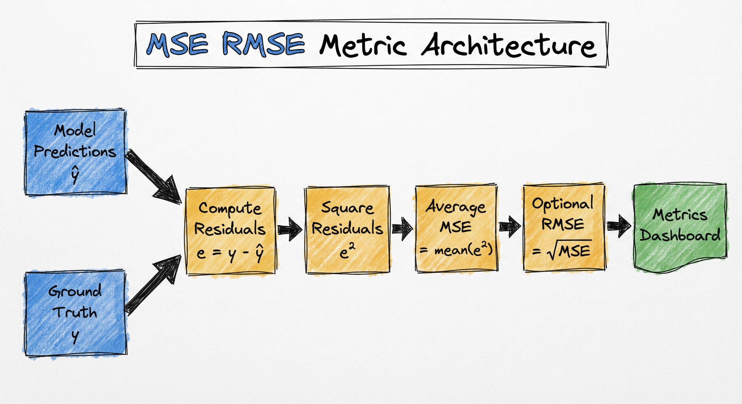
Evaluation Time: Model generates predictions -> predictions aligned with ground truth labels -> residuals computed -> squared -> averaged to produce MSE -> optionally square-rooted to produce RMSE -> logged to experiment tracking system.
Training Time (MSE as Loss): Forward pass produces predictions -> MSE loss computed -> backpropagation computes gradients -> optimizer updates weights -> repeat.
A linear flow from 'Model Predictions' and 'Ground Truth' → 'Compute Residuals' → 'Square Residuals' → 'Average (MSE)' → optional 'Square Root (RMSE)' → 'Metrics Dashboard'.
How to Implement
Implementation Patterns
Most practitioners use scikit-learn's mean_squared_error function, which handles edge cases and provides a battle-tested implementation. For deep learning, frameworks like PyTorch and TensorFlow include MSE as a built-in loss function optimized for GPU computation.
Manual Implementation: Occasionally necessary when integrating with custom pipelines or when you need to modify the metric (e.g., weighted MSE, sample-specific penalties).
Cost Note: MSE/RMSE computation is computationally cheap -- time and space for streaming computation. Even for millions of predictions, evaluation completes in milliseconds. The metric itself is never a bottleneck; the model inference that generates predictions is.
from sklearn.metrics import mean_squared_error
import numpy as np

# Ground truth and predictions
y_true = np.array([3.0, -0.5, 2.0, 7.0])
y_pred = np.array([2.5, 0.0, 2.0, 8.0])

# Compute MSE
mse = mean_squared_error(y_true, y_pred)
print(f"MSE: {mse:.4f}")  # Output: MSE: 0.3750

# Compute RMSE (two methods)
# Method 1: squared=False parameter
rmse = mean_squared_error(y_true, y_pred, squared=False)
print(f"RMSE (method 1): {rmse:.4f}")  # Output: RMSE: 0.6124

# Method 2: manual square root
rmse_manual = np.sqrt(mse)
print(f"RMSE (method 2): {rmse_manual:.4f}")  # Output: RMSE: 0.6124
The scikit-learn implementation handles edge cases like empty arrays and provides the squared parameter for direct RMSE computation. Note that squared=False was added in sklearn 0.23; older versions required manual sqrt(mse).
import torch
import torch.nn as nn

# Define model, loss, optimizer
model = nn.Linear(10, 1)  # simple linear regression
criterion = nn.MSELoss()
optimizer = torch.optim.SGD(model.parameters(), lr=0.01)

# Training loop (single step)
for epoch in range(100):
    # Forward pass
    outputs = model(X_train)
    loss = criterion(outputs, y_train)

    # Backward pass and optimize
    optimizer.zero_grad()
    loss.backward()  # Gradient of MSE is computed here
    optimizer.step()

    if epoch % 10 == 0:
        print(f"Epoch {epoch}, MSE Loss: {loss.item():.4f}")
PyTorch's nn.MSELoss() computes the mean of squared errors and is fully differentiable for backpropagation. The default reduction is 'mean'; you can also use 'sum' or 'none' for per-sample losses. The gradient computation is optimized for GPU execution.
import numpy as np

def mse(y_true, y_pred):
    """Compute Mean Squared Error."""
    if len(y_true) != len(y_pred):
        raise ValueError("Input arrays must have the same length")

    residuals = np.asarray(y_true) - np.asarray(y_pred)
    return np.mean(residuals ** 2)

def rmse(y_true, y_pred):
    """Compute Root Mean Squared Error."""
    return np.sqrt(mse(y_true, y_pred))

# Example: predicting house prices
y_true = np.array([45_00_000, 38_00_000, 52_00_000])  # INR
y_pred = np.array([43_50_000, 39_00_000, 51_00_000])  # INR

print(f"MSE: ₹{mse(y_true, y_pred):,.0f}²")
print(f"RMSE: ₹{rmse(y_true, y_pred):,.0f}")
# Output:
# MSE: ₹1,166,666,666,667²
# RMSE: ₹1,08,012
This manual implementation shows the core computation. Note the use of np.asarray() to handle list inputs and the explicit length check. For production, use sklearn's implementation which includes additional validation and optimizations.
import numpy as np

def weighted_mse(y_true, y_pred, sample_weights):
    """Compute weighted MSE where each sample has a custom weight."""
    residuals = y_true - y_pred
    squared_residuals = residuals ** 2
    weighted_errors = squared_residuals * sample_weights
    return np.sum(weighted_errors) / np.sum(sample_weights)

# Example: penalize errors on high-value samples more
y_true = np.array([100, 200, 300])
y_pred = np.array([110, 190, 310])
weights = np.array([1.0, 1.0, 2.0])  # double penalty for third sample

wmse = weighted_mse(y_true, y_pred, weights)
print(f"Weighted MSE: {wmse:.2f}")  # Output: 125.00
print(f"Standard MSE: {np.mean((y_true - y_pred) ** 2):.2f}")  # Output: 100.00
Weighted MSE is useful when samples have varying importance. For example, in e-commerce demand forecasting, errors during festive seasons might be weighted higher than regular days. The normalization by sum(weights) ensures the metric remains interpretable.
# Example: MLflow experiment tracking config
import mlflow

with mlflow.start_run():
    # Train model...
    predictions = model.predict(X_test)

    # Log metrics
    mse = mean_squared_error(y_test, predictions)
    rmse = mean_squared_error(y_test, predictions, squared=False)

    mlflow.log_metric("test_mse", mse)
    mlflow.log_metric("test_rmse", rmse)
    mlflow.log_param("metric_type", "regression")

    # Log for model comparison
    mlflow.sklearn.log_model(model, "model")
Common Implementation Mistakes
- ●
Computing MSE on the training set and claiming "my model is great" -- this is textbook overfitting diagnosis failure. ALWAYS evaluate MSE on held-out validation or test data that the model never saw during training.
- ●
Comparing MSE values across datasets or target variables with different scales. MSE on house prices (in crores) vs. apartment rent (in thousands) are not comparable. Use RMSE or standardized metrics instead.
- ●
Ignoring outliers before computing MSE -- a single extreme outlier can dominate the metric and give a misleading picture of model performance. Always visualize residuals and consider robust alternatives like MAE if outliers are present.
- ●
Using RMSE as a loss function in training instead of MSE -- while mathematically valid, RMSE's square root introduces numerical complexity in gradient computation and can slow convergence. Stick to MSE for training, use RMSE for evaluation.
- ●
Forgetting to take the square root when reporting RMSE -- I've seen this in production dashboards where teams report MSE but label it as RMSE, causing massive confusion when stakeholders interpret the units.
When Should You Use This?
Use When
Your error distribution is approximately normal (Gaussian) or you can assume it for simplicity
Large prediction errors are significantly more costly than small ones -- the quadratic penalty aligns with your business impact
You need a differentiable loss function for gradient-based optimization (neural networks, linear regression)
You want to leverage the bias-variance decomposition for model diagnostics
Computational efficiency matters and you need the simplest, fastest metric available
You're working with continuous regression targets like prices, temperatures, or counts where outliers are rare
Avoid When
Your dataset contains significant outliers that shouldn't dominate the metric -- consider MAE or Huber loss instead
All errors are equally important regardless of magnitude (e.g., delivery time estimation where being 10 minutes late is not 4x worse than 5 minutes late)
You need a metric that's robust to scale differences when comparing models trained on different target variables
Interpretability for non-technical stakeholders is critical -- RMSE helps but MAE is even simpler
Your error distribution is heavy-tailed (exponential, Laplacian) where MAE would be more statistically appropriate
Key Tradeoffs
MSE vs. RMSE: Which Should You Report?
Use MSE when:
- You're optimizing during training (it's the actual loss function)
- You're doing theoretical analysis (bias-variance decomposition)
- Computational simplicity matters (avoid the extra sqrt operation)
Use RMSE when:
- You're reporting to stakeholders who need interpretable units
- Comparing model performance across different scales
- Publishing results where readers expect error in original units
MSE vs. MAE: The Central Tradeoff
This is the big one. Here's a decision tree:
Choose MSE/RMSE if:
- Normal error distribution is a reasonable assumption
- Large errors are truly disproportionately bad
- You want convex optimization (guaranteed global minimum for linear models)
- You need fast gradient computation
Choose MAE if:
- You have outliers that shouldn't dominate the metric
- Errors are equally bad regardless of magnitude
- Robustness is more important than statistical efficiency
- Interpretability is critical ("average error is X units")
Computational Cost
MSE: time, space (streaming). Trivially parallelizable.
RMSE: Same as MSE plus one sqrt operation -- negligible cost.
For 1 million predictions, both compute in <10ms on a single CPU core. The metric computation is never your bottleneck.
Scale Sensitivity
Critical point: MSE is not scale-invariant. If you multiply your target variable by 10, MSE increases by 100x. This makes cross-dataset comparison difficult. Solutions:
- Use RMSE (only 10x increase)
- Use R² or MAPE (scale-invariant)
- Normalize targets before computing MSE
Production Tip: In Indian ML systems handling rupee amounts (house prices, loan defaults), always log both MSE and RMSE. Use MSE internally for optimization, report RMSE to business stakeholders in ₹ units they can understand.
Alternatives & Comparisons
MAE computes the average of absolute errors: mean(|y - ŷ|). It's more robust to outliers because it doesn't square errors, making all errors contribute linearly to the final metric. Use MAE when outliers exist or when all errors are equally bad. However, MAE's gradient is discontinuous at zero (absolute value is not differentiable at the origin), which can cause optimization issues. For evaluation, MAE is often preferable; for training, MSE is computationally superior.
R² measures the proportion of variance explained by the model: 1 - (SSE / SST). Unlike MSE/RMSE, R² is scale-invariant and always falls between 0 and 1 (or negative for terrible models), making it easier to interpret across different datasets. However, R² doesn't tell you the absolute magnitude of errors -- a model can have high R² but still make large errors if the target has high variance. Use R² for model comparison, MSE/RMSE for absolute error quantification.
MAPE expresses errors as percentages: mean(|y - ŷ| / |y|) × 100%. This makes it scale-invariant and intuitive for stakeholders ("the model is off by 5% on average"). However, MAPE breaks when ground truth values are zero or close to zero (division by zero), and it asymmetrically penalizes over-predictions less than under-predictions. Use MAPE for business reporting when targets are always positive and reasonably large.
Huber loss is MSE for small errors and MAE for large errors -- the best of both worlds. It's differentiable everywhere (unlike MAE) and robust to outliers (unlike MSE). The transition point δ is a hyperparameter. Use Huber loss when you have outliers but still need smooth gradients for optimization. Slightly more complex to implement and tune than pure MSE or MAE.
Pros, Cons & Tradeoffs
Advantages
Convex loss surface for linear models guarantees a global minimum -- no local minima traps, making optimization straightforward and predictable.
Differentiable everywhere with a simple linear gradient (∂MSE/∂w ∝ error), enabling efficient gradient descent and well-behaved backpropagation in neural networks.
Unique bias-variance decomposition (Bias² + Variance + Irreducible Error) allows diagnostic insights into whether your model suffers from underfitting or overfitting.
Corresponds to maximum likelihood estimation under Gaussian noise assumptions, giving it a solid statistical foundation beyond computational convenience.
Computationally extremely cheap -- time, space, trivially parallelizable. Evaluating 10 million predictions takes milliseconds.
RMSE returns errors in the original units of the target variable, making it interpretable for stakeholders (e.g., "predictions are off by ₹15,000 on average").
Heavily penalizes large errors via the quadratic term, naturally aligning with scenarios where big mistakes are disproportionately costly (financial forecasting, safety-critical systems).
Universally supported across all ML libraries -- sklearn, PyTorch, TensorFlow, XGBoost all provide optimized implementations.
Disadvantages
Extremely sensitive to outliers -- a single bad prediction can dominate the metric and make a good model look terrible. Outliers contribute quadratically, not linearly.
Not scale-invariant: MSE increases with the square of target scale, making cross-dataset comparisons difficult without normalization. A model predicting house prices vs. apartment rent will have incomparable MSE values.
The squared units (e.g., rupees²) are not interpretable for MSE, requiring the extra step of computing RMSE to return to meaningful units.
Assumes errors are symmetric -- penalizes over-predictions and under-predictions equally. In many applications (inventory management, medical diagnosis), asymmetric costs are the reality.
Implicitly assumes Gaussian error distribution. If your errors are heavy-tailed (Laplacian, Cauchy), MAE would be more statistically appropriate.
Can mask model performance issues when variance in the target is very high -- a model might have high MSE simply because the problem is inherently noisy, not because the model is bad.
Gradient can become very large for extreme errors, potentially causing instability in early training stages if not paired with gradient clipping or learning rate schedules.
Failure Modes & Debugging
Outlier domination
Cause
Dataset contains extreme outliers (data entry errors, rare events, measurement noise) that weren't cleaned during preprocessing. The squaring operation causes these outliers to contribute hundreds or thousands of times more to MSE than typical errors.
Symptoms
MSE/RMSE values are extremely high despite the model performing well on most samples. A single bad prediction in the test set causes the metric to skyrocket. Residual plots show a few extreme outliers far from the zero line while most points cluster near zero.
Mitigation
Visualize residuals before computing MSE/RMSE -- use residual plots and box plots to identify outliers. Consider robust alternatives like MAE or Huber loss if outliers are legitimate and can't be removed. Apply outlier detection (IQR, Z-score) during data cleaning. For training, use gradient clipping to prevent extreme gradients from destabilizing optimization.
Scale misinterpretation
Cause
MSE values are compared across models trained on differently-scaled target variables, or raw MSE (in squared units) is reported when RMSE (in original units) would be interpretable. Stakeholders see "MSE = 400,000,000" for house price prediction and think the model is terrible without realizing this is ₹20,000 RMSE.
Symptoms
Confusion during model comparison meetings. Teams waste time debating which model is better when the MSE values aren't comparable. Metrics dashboards show MSE in scientific notation, making interpretation impossible.
Mitigation
Always report RMSE alongside MSE for interpretability. For cross-dataset comparison, use scale-invariant metrics like R² or MAPE. Normalize targets to [0,1] or standardize to mean=0, std=1 before training, then compute MSE on the normalized scale. Clearly document the units in all reporting.
Training-test set leakage masking
Cause
Model is evaluated on the training set (or on test data that's too similar to training data) instead of a proper held-out set. MSE looks great because the model has memorized the training distribution, but generalization is poor.
Symptoms
Training MSE is extremely low (close to zero) while validation/test MSE is high. Large gap between train and test performance indicates overfitting. Stakeholders are confused when the "well-performing" model fails in production.
Mitigation
ALWAYS evaluate MSE/RMSE on a held-out test set that the model never saw during training. Use cross-validation to get a more robust estimate of generalization performance. Monitor the train-test MSE gap as a proxy for overfitting. Set up proper train-val-test splits: 70-15-15 or 60-20-20.
Non-Gaussian error distribution
Cause
Errors follow a heavy-tailed distribution (exponential, Laplacian, t-distribution) rather than Gaussian. MSE's assumption of normality is violated, making it statistically inefficient and prone to being dominated by rare large errors.
Symptoms
Histogram of residuals shows long tails or skewness instead of a bell curve. QQ-plots reveal deviations from normality. MSE is much higher than MAE, indicating the quadratic penalty is over-weighting tail errors.
Mitigation
Plot residual distribution (histogram, QQ-plot) to diagnose normality. If errors are heavy-tailed, switch to MAE which is optimal for Laplacian errors. For intermediate cases, use Huber loss with an appropriate δ threshold. Consider quantile regression if different parts of the distribution need different models.
Numerical overflow in large-scale systems
Cause
When predictions and targets are very large (e.g., GDP in rupees, astronomical distances), squaring can cause float32 overflow, producing NaN or Inf values. Alternatively, summing millions of squared errors can exceed floating-point precision.
Symptoms
MSE computation returns NaN or Inf. Training loss suddenly jumps to NaN mid-epoch. Gradient updates become erratic. Logs show floating-point overflow warnings.
Mitigation
Use float64 (double precision) instead of float32 for metric computation if values are large. Normalize targets to a reasonable scale (e.g., house prices in lakhs instead of raw rupees) before training. For distributed systems, use numerically stable reduction algorithms (Kahan summation). Check for overflow explicitly: if mse > 1e15, investigate before proceeding.
Placement in an ML System
Where Does It Sit in the Pipeline?
In a training pipeline, MSE serves as the loss function that guides optimization. It's computed after every forward pass, gradients are derived from it, and those gradients update model weights.
In an evaluation pipeline, MSE/RMSE are computed after the model generates predictions on validation or test sets. They're logged to experiment tracking systems (MLflow, Weights & Biases), displayed on dashboards, and used for model selection.
In a production monitoring pipeline, RMSE is computed on incoming predictions vs. actual outcomes (when labels arrive later) to detect model drift. For example, in e-commerce demand forecasting, you predict tomorrow's sales, then compute RMSE once actual sales are known 24 hours later.
Production Pattern: Log MSE during training (it's the optimization objective), log RMSE during evaluation (it's interpretable), and monitor RMSE in production (it's scale-agnostic and stakeholder-friendly). This three-stage pattern is nearly universal in regression systems.
Pipeline Stage
Evaluation / Monitoring
Upstream
- Trained Model
- Prediction Generator
- Test Data Loader
Downstream
- Metrics Dashboard
- Model Selection Logic
- Hyperparameter Tuning System
- A/B Testing Framework
Scaling Bottlenecks
MSE/RMSE computation itself is almost never a bottleneck -- it's and embarrassingly parallelizable. The real bottlenecks are upstream:
Prediction generation: If your model takes 100ms per inference and you have 1 million test samples, that's 100,000 seconds (27 hours) just to generate predictions. The 10ms to compute MSE is negligible.
Data loading: For large test sets stored in cloud storage, I/O can dominate. Fetching 1GB of predictions and labels from S3 takes longer than computing MSE.
Distributed aggregation: In distributed evaluation (Spark, Dask), the reduce operation to sum squared errors across nodes introduces network overhead. Use tree reduction rather than naive all-reduce.
For 1 billion predictions:
- Single-threaded Python: ~5 seconds
- Vectorized NumPy: ~500ms
- GPU (CUDA): ~50ms
- Distributed (100 nodes): ~100ms including network overhead
The metric scales linearly with data size, so doubling your test set doubles computation time -- no surprises.
Production Case Studies
Uber's marketplace forecasting enables prediction of user supply and demand in spatio-temporal fine granular fashion. The system uses RMSE (Root Mean Squared Error) to evaluate forecast accuracy for directing driver-partners to high demand areas before they arise.
Uber's forecasting system increases driver trip counts and earnings by accurately predicting demand patterns. The spatio-temporal forecasts help optimize marketplace efficiency by proactively positioning drivers in areas that will experience high demand.
Zillow's Zestimate home valuation model predicts house prices using a machine learning pipeline that considers property attributes, location, market trends, and historical sales. The model is evaluated primarily using median absolute error and RMSE. For high-value properties, large errors are exponentially more damaging to reputation and user trust -- a 2M home is worse than a 200K home in terms of business impact.
Zillow reports a median error rate (similar to MAE) of about 2.4% for on-market homes and uses RMSE internally to detect when the model makes catastrophic errors. The focus on both metrics balances robustness (MAE) with sensitivity to large mistakes (RMSE). When RMSE spikes relative to MAE, it signals outlier predictions that need manual review.
BigBasket uses machine learning to forecast product demand at the SKU level across warehouses. The regression models predict daily demand (number of units) for thousands of products. RMSE is used as the primary evaluation metric because stockouts (under-prediction) and excess inventory (over-prediction) both have costs, but large errors are disproportionately expensive -- predicting 10 units when demand is 100 causes lost sales and customer dissatisfaction.
By optimizing demand forecasting models to minimize RMSE, BigBasket reduced inventory holding costs by approximately 8% while maintaining service levels. The RMSE metric helped identify categories (perishables, seasonal items) where prediction errors were highest and needed targeted model improvements.
DeepMind developed neural networks to predict data center cooling requirements (measured in power usage effectiveness, PUE). The models predict a continuous target (future PUE) and are optimized using MSE loss. The predictions guide automatic adjustments to cooling systems. Large prediction errors could cause either overheating (catastrophic) or energy waste (expensive), making RMSE an appropriate metric.
The ML system achieved a 40% reduction in cooling costs by accurately predicting and optimizing PUE. The model's RMSE on validation data was reported as 0.004 PUE, which translates to extremely accurate predictions that enabled safe automation of cooling controls.
Tooling & Ecosystem
The standard library for MSE and RMSE computation in Python. Provides mean_squared_error() with squared=False option for RMSE. Supports multioutput regression and sample weights. Battle-tested, optimized, and handles edge cases (empty arrays, NaN values).
Deep learning framework with nn.MSELoss() as a built-in loss function. Fully differentiable for backpropagation, GPU-accelerated, and integrates seamlessly with PyTorch training loops. Supports different reduction modes (mean, sum, none).
Provides tf.keras.losses.MeanSquaredError() for training and tf.keras.metrics.RootMeanSquaredError() for evaluation. GPU-optimized, supports distributed training, and integrates with TensorBoard for visualization.
Gradient boosting library that uses squared error ('reg:squarederror') as the default objective for regression tasks. Internally optimizes MSE during tree construction. Supports custom evaluation metrics including RMSE via eval_metric parameter.
Experiment tracking platform that logs and visualizes metrics including MSE and RMSE across training runs. Enables comparison of models by sorting runs by RMSE. Integrates with scikit-learn, PyTorch, and TensorFlow.
ML experiment tracking with built-in support for logging and plotting regression metrics. Automatically computes and visualizes RMSE over epochs. Provides dashboards for comparing RMSE across multiple models and hyperparameter configurations.
Distributed machine learning library with RegressionEvaluator that computes RMSE, MSE, MAE, and R² at scale. Optimized for evaluating models on massive datasets across Spark clusters.
Research & References
Chai, T. & Draxler, R.R. (2014)Geoscientific Model Development, Vol. 7
A seminal paper defending RMSE against claims that it should be avoided due to outlier sensitivity. The authors argue that RMSE is appropriate when large errors are indeed more problematic than small ones and that its mathematical properties (convexity, decomposability) justify its continued use. They emphasize that metric choice should align with the error distribution and cost structure of the problem.
Stanford Encyclopedia of Philosophy (2024)Stanford Encyclopedia of Philosophy
Comprehensive theoretical treatment of the bias-variance decomposition: E[MSE] = Bias² + Variance + Irreducible Error. Explains why this decomposition is fundamental to understanding the underfitting-overfitting tradeoff and why it doesn't extend cleanly to other loss functions like MAE.
Willmott, C.J., Robeson, S.M. & Matsuura, K. (2023)PLOS ONE, Vol. 18, No. 2
Develops a decomposition of MAE analogous to MSE's bias-variance decomposition, breaking it into bias error, proportionality error, and unsystematic error. Argues that MAE decomposition provides more interpretable components than MSE decomposition in the presence of outliers or non-normal error distributions.
Friedman, J.H. (2001)Statistical Science, Vol. 16, No. 1
Explains why minimizing MSE is equivalent to maximum likelihood estimation under Gaussian error assumptions. This statistical foundation justifies MSE's use beyond computational convenience and connects classical least squares to modern probabilistic modeling.
Zhang, Y. et al. (2025)Premier Journal of AI Research
Reviews regression metrics (MSE, RMSE, MAE, MAPE, R²) in the context of energy demand forecasting. Discusses why RMSE is preferred in forecasting competitions due to its ability to reflect accuracy across different models and datasets while penalizing large errors that are particularly costly in grid management.
Trevisan, V. (2020)Towards Data Science
Empirical study comparing MAE, MSE, and RMSE under varying outlier intensities and frequencies. Demonstrates that MSE/RMSE distributions shift significantly more than MAE when outliers are present, confirming that MAE is more robust. Provides quantitative guidance on when to prefer each metric based on dataset characteristics.
Cho, K. et al. (2014)SSST-8, Eighth Workshop on Syntax, Semantics and Structure in Statistical Translation
While focused on NLP, this paper discusses the use of MSE (and related squared loss functions) in sequence-to-sequence models. Highlights computational benefits of quadratic loss for backpropagation through time (BPTT) and the importance of gradient smoothness for training deep networks.
Interview & Evaluation Perspective
Common Interview Questions
- ●
What is the difference between MSE and RMSE? When would you use one over the other?
- ●
Why is MSE commonly used as a loss function rather than MAE?
- ●
Explain the bias-variance decomposition of MSE.
- ●
How does MSE handle outliers compared to MAE?
- ●
Can you derive the gradient of MSE for a linear regression model?
- ●
What are the assumptions behind using MSE as an evaluation metric?
- ●
How would you detect if MSE is being dominated by outliers in your dataset?
Key Points to Mention
- ●
MSE squares errors, making it sensitive to outliers and giving large errors disproportionate weight. RMSE takes the square root to return to original units, improving interpretability.
- ●
MSE is preferred as a loss function because its gradient is linear in the error (∂MSE/∂w ∝ error), making gradient descent stable and efficient. MAE's gradient is constant (non-zero errors all have the same gradient), which can slow convergence.
- ●
The bias-variance decomposition (E[MSE] = Bias² + Variance + Irreducible Error) is unique to MSE and provides diagnostic value for understanding underfitting vs. overfitting.
- ●
Under Gaussian error assumptions, minimizing MSE is equivalent to maximum likelihood estimation -- this statistical foundation is more than just computational convenience.
- ●
MSE is not scale-invariant: if you multiply your target by 10, MSE increases by 100x. This makes cross-dataset comparison difficult without normalization.
Pitfalls to Avoid
- ●
Claiming MSE and RMSE are "better" than MAE without qualifying the context -- the right metric depends on error distribution and cost structure. Don't make blanket statements.
- ●
Confusing MSE (squared units) with RMSE (original units) when interpreting values -- saying "MSE is 400 million" for house prices sounds terrible, but RMSE of ₹20,000 might be acceptable.
- ●
Forgetting that MSE is extremely outlier-sensitive and not mentioning the need to inspect residuals before trusting MSE-based conclusions.
- ●
Saying "MSE is convex" without clarifying you mean the loss landscape is convex for linear models -- for neural networks, the overall loss landscape is non-convex even if the loss function is quadratic.
- ●
Not mentioning that MSE assumes symmetric error costs -- in many real-world problems (medical diagnosis, inventory management), asymmetric costs require custom loss functions.
Senior-Level Expectation
A senior candidate should be able to discuss not just the mechanics of MSE/RMSE computation, but the deeper considerations: when to use MSE vs. MAE from first principles (Gaussian vs. Laplacian error distributions, maximum likelihood perspective), how to diagnose outlier sensitivity (residual plots, comparing MSE/MAE ratio), the trade-off between interpretability (RMSE) and optimization efficiency (MSE), and how to handle edge cases in production (numerical stability, scale normalization, weighted MSE for imbalanced regression). The ability to connect the choice of metric to business impact -- explaining why RMSE's quadratic penalty aligns with cost structures in financial forecasting or demand planning -- separates senior practitioners from junior ones.
Summary
Let's recap the essentials:
-
MSE and RMSE measure prediction error by averaging the squared differences between predictions and actual values. MSE is in squared units; RMSE takes the square root to return to original units for interpretability.
-
The quadratic penalty from squaring errors means large mistakes are disproportionately costly. An error of 10 contributes 100 to MSE, while an error of 20 contributes 400 -- this aligns with many real-world scenarios where big errors are exponentially worse than small ones.
-
MSE is the workhorse loss function for regression because its gradient is simple and linear in the error: ∂MSE/∂w ∝ (ŷ - y). This makes gradient descent efficient and the loss landscape convex for linear models.
-
The bias-variance decomposition (E[MSE] = Bias² + Variance + Irreducible Error) is unique to MSE and provides diagnostic insights into underfitting vs. overfitting that other metrics can't offer.
-
Outlier sensitivity is MSE's biggest weakness. A single extreme error can dominate the metric. Always visualize residuals and consider MAE or Huber loss if outliers are present and legitimate.
-
Use MSE for training (optimization efficiency), RMSE for reporting (interpretability), and both for evaluation (comprehensive view). Compare against MAE to detect outlier influence.
MSE and RMSE are the default regression metrics for good reason: they're computationally efficient, theoretically grounded (maximum likelihood under Gaussian errors), and align with scenarios where large errors are disproportionately problematic. But they're not universal -- always validate that the quadratic penalty matches your problem's cost structure and that outliers aren't skewing your conclusions.