What is the difference between MAE and RMSE, and when should I use each?

MAE (Mean Absolute Error) and RMSE (Root Mean Squared Error) differ in how they penalize errors. MAE uses a **linear penalty**: an error of 10 contributes exactly twice as much as an error of 5. RMSE uses a **quadratic penalty** (via squaring before averaging): an error of 10 contributes four times as much as an error of 5, making RMSE much more sensitive to outliers. **Use MAE when**: (1) You want robustness to outliers—occasional large errors shouldn't dominate your metric. (2) Interpretability matters—stakeholders understand "predictions are off by ₹500 on average." (3) You care about typical performance rather than worst-case scenarios. (4) You want to predict medians (for skewed distributions). **Use RMSE when**: (1) Large errors are particularly costly or dangerous (medical, financial, safety-critical systems). (2) You want to optimize for the mean rather than the median. (3) Smooth gradients are important for optimization (RMSE is differentiable everywhere, MAE is not at zero). (4) You want to penalize variance in predictions more heavily. In practice, **report both**: if RMSE >> MAE, you have significant outliers. If RMSE ≈ MAE, your errors are relatively uniform. The ratio RMSE/MAE provides insight into error distribution shape.

Why does minimizing MAE during training yield median predictions instead of mean predictions?

This is a fundamental result from robust statistics. The value $\hat{y}$ that minimizes $\sum |y_i - \hat{y}|$ (the sum of absolute deviations) is the **median** of $\{y_1, y_2, \ldots, y_n\}$, while the value that minimizes $\sum (y_i - \hat{y})^2$ (the sum of squared deviations) is the **mean**. Intuitively, the median is the "middle" value that balances the number of points above and below it, minimizing total movement (L1 distance). The mean minimizes total squared movement (L2 distance), which pulls toward extreme values more strongly due to squaring. In machine learning, this means: when you train a regression model with **MAE loss**, the model learns to predict the **conditional median** of the target given the input features: median(y | X). When you train with **MSE loss**, it predicts the **conditional mean**: E[y | X]. Why does this matter? For **skewed distributions** (income, housing prices, demand with spikes), the median is often more representative than the mean. The mean is pulled by outliers; the median is robust. For example, if predicting salaries in a company where most earn ₹8-12 lakhs but a few executives earn ₹2 crores, the mean salary might be ₹18 lakhs (unrepresentative), while the median stays around ₹10 lakhs (typical). MAE-trained models would predict values closer to ₹10 lakhs for most employees, while MSE-trained models might overpredict due to the high-earner tail.

How can I make MAE comparable across datasets with different target scales?

MAE is **scale-dependent**: an MAE of 100 is meaningless without knowing whether you're predicting rupees (small), kilograms (medium), or distance in meters (large). To compare MAE across datasets or targets with different scales, use these normalization strategies: **1. Percentage of Mean (MAE / mean(y_true))**: Expresses MAE as a fraction of the average target value. Example: MAE = ₹5000 on house prices averaging ₹50 lakhs → 1% error. Simple but sensitive to near-zero means. **2. MAPE (Mean Absolute Percentage Error)**: Computes `mean(|y_true - y_pred| / y_true) × 100%`. Scale-free and intuitive ("10% error on average"), but **fails when y_true contains zeros** and is asymmetric (penalizes under-prediction more than over-prediction). **3. Normalized MAE (MAE / std(y_true))**: Divides MAE by the standard deviation of the target. Expresses error as a multiple of typical variation. Works well for comparing across datasets. **4. Normalized MAE by Range (MAE / (max(y_true) - min(y_true)))**: Useful when the target has a fixed range (e.g., ratings from 1-5). Expresses MAE as a fraction of the total scale. **5. Relative MAE (MAE / baseline_MAE)**: Compare your model's MAE to a simple baseline (e.g., always predicting the mean or median). MAE_model / MAE_baseline < 1 means your model beats the baseline. For cross-dataset comparisons, **MAPE** is most common (when targets are strictly positive), followed by percentage-of-mean. Always report both absolute MAE (for interpretability) and normalized MAE (for comparison) when presenting results.

What is Median Absolute Error (MedAE), and when should I use it instead of MAE?

**Median Absolute Error (MedAE)** is computed by taking the **median** of absolute errors instead of the mean: `median(|y_true - y_pred|)`. While MAE averages all errors, MedAE selects the middle value, making it **extremely robust to outliers**—even more so than MAE. Mathematically: MAE = mean(|errors|), MedAE = median(|errors|). A single outlier increases MAE linearly (contributing to the sum), but doesn't affect MedAE unless more than 50% of predictions are outliers (the median only cares about rank order, not magnitude). **When to use MedAE**: - **Heavy outlier contamination**: If your data has frequent extreme errors (e.g., production anomalies, sensor failures), MedAE is unaffected while MAE inflates. - **Diagnosing MAE inflation**: Compute both MAE and MedAE. If MAE >> MedAE (ratio > 2), you have significant outliers skewing the average. This ratio is a valuable signal for data quality monitoring. - **Reporting typical errors**: MedAE answers "what is the error for the typical prediction?" better than MAE in skewed distributions. **Example**: Predictions have errors [1, 2, 3, 4, 1000]. MAE = 202 (dominated by the outlier), MedAE = 3 (unaffected). The ratio MAE/MedAE = 67 immediately flags outlier influence. In production systems, many teams report **MAE, MedAE, and their ratio** as a standard metric triple. Scikit-learn provides `sklearn.metrics.median_absolute_error()` for easy computation. The tradeoff: MedAE is harder to optimize during training (non-differentiable and more complex than MAE) and doesn't aggregate nicely across groups (median(A ∪ B) ≠ median(A) + median(B)).

How do I implement MAE for streaming data or production monitoring?

For **streaming MAE** in production systems (where predictions arrive continuously and you can't store all history), use a **running statistics** approach: **Basic streaming MAE** (unbounded window): ```python class StreamingMAE: def __init__(self): self.sum_errors = 0.0 self.count = 0 def update(self, y_true, y_pred): error = abs(y_true - y_pred) self.sum_errors += error self.count += 1 def compute(self): return self.sum_errors / self.count if self.count > 0 else 0.0 def reset(self): self.sum_errors = 0.0 self.count = 0 ``` This maintains only two values in memory (sum, count) regardless of stream length. Update complexity: O(1), compute complexity: O(1). **Sliding window MAE** (e.g., "MAE over last 10,000 predictions"): - Use a **circular buffer** (collections.deque with maxlen) to store recent errors. - Recompute MAE = mean(buffer) on demand. - Memory: O(window_size), update: O(1), compute: O(window_size). **Time-based windows** (e.g., "MAE over last 24 hours"): - Store (timestamp, error) tuples in a time-indexed data structure. - On compute, filter errors within [now - 24h, now] and average. - For efficiency, use bucketing: maintain MAE per hour, then aggregate. **Distributed streaming** (Kafka, Flink, Spark Streaming): - Compute partial sums and counts per partition/worker. - Aggregate via a reduce operation: global_sum = sum(partial_sums), global_count = sum(partial_counts), MAE = global_sum / global_count. - For time-based windows, use event time processing with watermarks. **Integration with monitoring stacks**: - **Prometheus**: Expose MAE as a gauge metric, updated periodically. Use recording rules for windowed aggregation. - **CloudWatch/Datadog**: Emit MAE as a custom metric every N minutes. Set alarms on thresholds. - **MLflow/W&B**: Log MAE at inference time using tracking APIs. **Best practices**: (1) Compute MAE at multiple granularities (per user segment, per product, global) to detect drift. (2) Pair with MedAE and percentile errors to catch outliers. (3) Use exponential smoothing for noisy MAE signals: smoothed_mae = alpha × new_mae + (1 - alpha) × smoothed_mae.

What is the relationship between MAE and quantile loss?

**Quantile loss** (also called **pinball loss**) is a generalization of MAE that allows asymmetric penalties for over- and under-prediction. While MAE treats +10 and -10 errors equally, quantile loss lets you penalize one direction more than the other, enabling **probabilistic forecasting** and prediction intervals. Quantile loss for quantile $\tau \in (0, 1)$ is defined as: $$L_\tau(y, \hat{y}) = \begin{cases} \tau \cdot (y - \hat{y}) & \text{if } y \geq \hat{y} \\ (1 - \tau) \cdot (\hat{y} - y) & \text{if } y < \hat{y} \end{cases}$$ Or more compactly: $L_\tau = \max(\tau \cdot (y - \hat{y}), (1 - \tau) \cdot (\hat{y} - y))$. **Special case: MAE is quantile loss at τ = 0.5** (the median): - When $\tau = 0.5$, the loss becomes $0.5 \cdot |y - \hat{y}|$, which is proportional to MAE. - Minimizing MAE is equivalent to minimizing the 50th percentile (median) quantile loss. **Use cases for quantile loss**: - **Asymmetric costs**: For inventory forecasting, under-prediction (stockouts) might be more costly than over-prediction (excess inventory). Use $\tau = 0.7$ to penalize under-prediction more. - **Prediction intervals**: Train models for $\tau = 0.1$ and $\tau = 0.9$ to get the 10th and 90th percentile predictions, forming an 80% prediction interval. - **Risk management**: In finance, you might care more about predicting the 5th percentile (Value at Risk) than the mean. **Example**: In demand forecasting, predicting too low (stockout) costs ₹100/unit, while predicting too high (overstock) costs ₹20/unit. Set $\tau = 0.83$ (approximately 100/(100+20)) to balance these asymmetric costs. Libraries like **LightGBM, XGBoost, and TensorFlow** support quantile loss directly. For multiple quantiles, train separate models or use a multi-output architecture.

How does Huber loss relate to MAE, and when should I use it?

**Huber loss** is a **hybrid** between MAE (L1 loss) and MSE (L2 loss), designed to combine MAE's robustness to outliers with MSE's smooth gradients for optimization. It behaves like MSE for small errors (quadratic, smooth) and like MAE for large errors (linear, robust). Huber loss is defined as: $$L_\delta(y, \hat{y}) = \begin{cases} \frac{1}{2}(y - \hat{y})^2 & \text{if } |y - \hat{y}| \leq \delta \\ \delta \cdot (|y - \hat{y}| - \frac{1}{2}\delta) & \text{otherwise} \end{cases}$$ where $\delta$ is a threshold parameter (tunable hyperparameter). **How it works**: For errors smaller than $\delta$, Huber uses squared loss (like MSE), providing smooth gradients near zero—helpful for optimization convergence. For errors larger than $\delta$, it switches to absolute loss (like MAE), preventing outliers from dominating the loss. **Comparison**: - **MAE**: Fully linear, non-differentiable at zero, robust to all outliers. - **MSE**: Fully quadratic, smooth everywhere, sensitive to all outliers. - **Huber**: Quadratic near zero (smooth), linear far from zero (robust). Differentiable everywhere (unlike MAE). **When to use Huber loss**: - **Training neural networks**: Huber provides better gradient flow than MAE (no non-differentiability at zero) while maintaining robustness to large errors. - **Outlier-contaminated data**: When you have some outliers but still want to penalize large errors more than MAE does, Huber finds a middle ground. - **Tuning robustness**: By adjusting $\delta$, you control the transition point between quadratic and linear behavior. Small $\delta$ → more like MAE (robust), large $\delta$ → more like MSE (sensitive). **Choosing δ**: Typical strategies: (1) Set $\delta$ = 1.0 (default in many libraries). (2) Set $\delta$ based on error percentiles (e.g., 90th percentile of training errors). (3) Treat as a hyperparameter and tune via cross-validation. **Libraries**: Available in TensorFlow (`tf.keras.losses.Huber`), PyTorch (`torch.nn.HuberLoss`), scikit-learn (`sklearn.linear_model.HuberRegressor` for robust regression). For evaluation, use MAE; for training, consider Huber if optimization struggles with MAE's non-smoothness.

Why might MAE and business metrics diverge, and how do I align them?

A common pitfall in production ML systems is optimizing for MAE while **business metrics** (revenue, customer satisfaction, operational costs) move in the opposite direction. This divergence happens because MAE treats all errors equally, but in reality, different errors have different business impacts. **Why divergence occurs**: 1. **Asymmetric costs**: In inventory forecasting, under-prediction (stockouts) loses revenue, while over-prediction incurs holding costs. MAE treats both equally, but stockouts might be 5× more costly. Your model might achieve low MAE by balancing errors, but business suffers from too many stockouts. 2. **Heterogeneous importance**: In demand forecasting across products, predicting a staple item (milk, 10,000 units/day) accurately matters more than a niche item (specialty spice, 10 units/day). But MAE treats a 10-unit error the same regardless of product. A model with low global MAE might have terrible accuracy on high-revenue products. 3. **Non-linear utility**: For ETA prediction, being 5 minutes late is annoying, but 30 minutes late causes cancellations. The business impact is non-linear, while MAE treats 30-minute errors as just 6× worse than 5-minute errors (linear). 4. **Temporal importance**: Errors during peak hours (lunch rush for food delivery) have higher operational impact than off-peak errors, but MAE weighs all timestamps equally. **How to align MAE with business metrics**: - **Weighted MAE**: Assign sample weights proportional to business impact. For inventory, weight samples by revenue per unit. For customers, weight by customer lifetime value (VIP customers get higher weights). Formula: $\text{MAE}_w = \frac{\sum w_i |y_i - \hat{y}_i|}{\sum w_i}$. - **Segment-specific MAE**: Compute MAE separately for high-impact vs. low-impact segments. Report both global MAE and per-segment MAE. Set tighter thresholds for critical segments. - **Cost-sensitive metrics**: Replace MAE with a custom metric that mirrors business costs. Example: $\text{Cost} = \sum_{i} c_i \cdot |y_i - \hat{y}_i|$ where $c_i$ is the cost per unit error for sample $i$. - **Quantile loss for asymmetric costs**: If under-prediction is 3× costlier, use quantile loss with $\tau = 0.75$ instead of MAE ($\tau = 0.5$). - **Multi-objective optimization**: Optimize a weighted combination of MAE and business-specific constraints (e.g., stockout rate < 2%, holding costs < ₹1 lakh/day). **Example (Swiggy)**: Their demand forecasting initially optimized for MAE, but this didn't prevent simultaneous stockouts (lost revenue) and overstock (waste). They implemented **adaptive metric alignment**, using weighted MAE where weights reflected operational impact, plus explicit constraints on stockout and waste rates. This aligned ML metrics with business objectives. **Recommendation**: Always validate MAE against real business KPIs during A/B tests. If model A has lower MAE but model B has higher revenue, investigate which errors matter most and adjust your metric accordingly.

Evaluation

MAE in Machine Learning

Q: What is Median Absolute Error (MedAE), and when should I use it instead of MAE?

**Median Absolute Error (MedAE)** is computed by taking the **median** of absolute errors instead of the mean: `median(|y_true - y_pred|)`. While MAE averages all errors, MedAE selects the middle value, making it **extremely robust to outliers**—even more so than MAE. Mathematically: MAE = mean(|errors|), MedAE = median(|errors|). A single outlier increases MAE linearly (contributing to the sum), but doesn't affect MedAE unless more than 50% of predictions are outliers (the median only cares about rank order, not magnitude). **When to use MedAE**: - **Heavy outlier contamination**: If your data has frequent extreme errors (e.g., production anomalies, sensor failures), MedAE is unaffected while MAE inflates. - **Diagnosing MAE inflation**: Compute both MAE and MedAE. If MAE >> MedAE (ratio > 2), you have significant outliers skewing the average. This ratio is a valuable signal for data quality monitoring. - **Reporting typical errors**: MedAE answers "what is the error for the typical prediction?" better than MAE in skewed distributions. **Example**: Predictions have errors [1, 2, 3, 4, 1000]. MAE = 202 (dominated by the outlier), MedAE = 3 (unaffected). The ratio MAE/MedAE = 67 immediately flags outlier influence. In production systems, many teams report **MAE, MedAE, and their ratio** as a standard metric triple. Scikit-learn provides `sklearn.metrics.median_absolute_error()` for easy computation. The tradeoff: MedAE is harder to optimize during training (non-differentiable and more complex than MAE) and doesn't aggregate nicely across groups (median(A ∪ B) ≠ median(A) + median(B)).

Mean Absolute Error (MAE) is one of the most intuitive and widely used metrics for evaluating regression models. Unlike its cousin MSE (Mean Squared Error), MAE measures the average magnitude of prediction errors using absolute values, making it robust to outliers and easy to interpret. Because MAE is expressed in the same units as the target variable, it provides a straightforward answer to the question: "On average, how far off are my predictions?" This interpretability makes MAE particularly valuable in production systems where stakeholders need to understand model performance without statistical expertise. Whether you're forecasting delivery times, predicting product prices, or estimating demand, MAE offers a linear, symmetric, and actionable view of your model's accuracy.

Concept Snapshot

What It Is: A regression metric that calculates the average absolute difference between predicted and actual values, providing an interpretable measure of prediction error magnitude.
Category: Evaluation
Complexity: Beginner
Inputs / Outputs: Predictions array + ground truth array → single MAE score (non-negative float, 0 is perfect)
System Placement: Post-prediction evaluation stage in training, validation, and production monitoring pipelines
Also Known As: Mean Absolute Deviation, L1 Loss, L1 Error, Average Absolute Error
Typical Users: Data Scientists, ML Engineers, Business Analysts, Product Managers, MLOps Engineers
Prerequisites: Basic statistics (mean, absolute value), Understanding of regression tasks, Familiarity with prediction vs ground truth
Key Terms: absolute errorresidualsL1 normrobust metricslinear lossmedian forecastingquantile lossoutlier sensitivity

Why This Concept Exists

MAE emerged from the fundamental need to quantify prediction accuracy in a way that's both mathematically sound and practically interpretable. Early statisticians working with regression problems in the 18th and 19th centuries—including luminaries like Laplace and Gauss—explored different ways to aggregate errors. While Gauss famously championed squared errors (leading to least squares regression), Laplace advocated for absolute deviations, recognizing their robustness to outliers and computational simplicity.

The historical tension between L1 (absolute) and L2 (squared) norms reflects different philosophical approaches to error measurement. Squared errors penalize large mistakes disproportionately, making them sensitive to outliers but analytically convenient (differentiable everywhere). Absolute errors treat all deviations linearly, making them more robust but historically harder to optimize due to non-differentiability at zero. With modern computational power, this optimization challenge has become negligible, and MAE has gained popularity for its intuitive interpretation.

In modern machine learning, MAE addresses a critical gap: stakeholder comprehension. When you tell a logistics manager that your delivery time model has an MAE of 8 minutes, they immediately understand the practical impact—predictions are off by 8 minutes on average. Compare this to explaining an MSE of 147 (square minutes?), and the value of MAE becomes clear. As ML systems moved from research labs to production environments serving non-technical stakeholders, interpretable metrics like MAE became essential tools for communicating model performance, setting SLAs, and making data-driven decisions about model deployment.

Core Intuition & Mental Model

Think of MAE as measuring the "typical miss distance" of your predictions. Imagine you're throwing darts at a target—MAE tells you the average distance from the bullseye, regardless of direction. A dart 5 cm north of center and a dart 5 cm south contribute equally to your MAE of 5 cm. This symmetry makes MAE fair: underestimating by ₹100 is just as bad as overestimating by ₹100.

The "absolute" part is crucial. Without it, positive and negative errors would cancel out, giving you a false sense of accuracy. If your model predicts ₹1000 for a product actually worth ₹1200, and ₹1400 for a product worth ₹1200, the raw errors (+200 and -200) cancel to zero—suggesting perfect accuracy when you're consistently off by ₹200. The absolute value prevents this cancellation, forcing you to acknowledge every mistake.

Here's the key insight about MAE's relationship to outliers: MAE treats all errors with equal importance on a linear scale. If you have 99 predictions with 1% error and one catastrophic outlier with 1000% error, MAE increases linearly by adding that outlier's contribution. In contrast, MSE/RMSE would square that 1000% error, dominating the entire metric. This makes MAE ideal when you care about typical performance rather than worst-case scenarios. A famous result from statistical theory: minimizing MAE during training produces a model that predicts the median of the target distribution, while minimizing MSE produces predictions of the mean. In skewed distributions (common in real-world data like income, housing prices, or delivery times), medians are often more representative and robust than means.

Technical Foundations

Mean Absolute Error is defined mathematically as:

$\text{MAE} = \frac{1}{n} \sum_{i=1}^{n} |y_i - \hat{y}_i|$

where:

$n$ is the number of samples
$y_i$ is the true value for sample $i$
$\hat{y}_i$ is the predicted value for sample $i$
$|\cdot|$ denotes the absolute value (L1 norm)

Properties:

Range: $\text{MAE} \in [0, \infty)$ , with 0 indicating perfect predictions
Scale dependency: MAE has the same units as the target variable $y$
Symmetry: $|y - \hat{y}| = |\hat{y} - y|$ , so overestimation and underestimation are penalized equally
Linearity: Errors contribute linearly to the total; doubling an error doubles its contribution
Convexity: MAE is a convex function, guaranteeing a unique global minimum
Non-differentiability: The absolute value function is not differentiable at zero, though subgradient methods handle this in practice

Relationship to L1 Norm:

MAE is equivalent to the L1 norm of the residual vector $\mathbf{r} = \mathbf{y} - \hat{\mathbf{y}}$ :

$\text{MAE} = \frac{1}{n} \|\mathbf{r}\|_1 = \frac{1}{n} \sum_{i=1}^{n} |r_i|$

Median Property:

A fundamental result from robust statistics: the value $\hat{y}$ that minimizes $\sum_{i=1}^{n} |y_i - \hat{y}|$ is the median of $\{y_1, y_2, \ldots, y_n\}$ . This means models trained with MAE loss tend to predict conditional medians rather than conditional means.

Weighted MAE:

For imbalanced or importance-weighted scenarios:

$\text{MAE}_w = \frac{\sum_{i=1}^{n} w_i |y_i - \hat{y}_i|}{\sum_{i=1}^{n} w_i}$

where $w_i$ are sample weights.

Computational Complexity:

Calculating MAE requires $O(n)$ operations: one subtraction, one absolute value, and one accumulation per sample, followed by division by $n$ . This makes MAE extremely efficient even for large-scale evaluation.

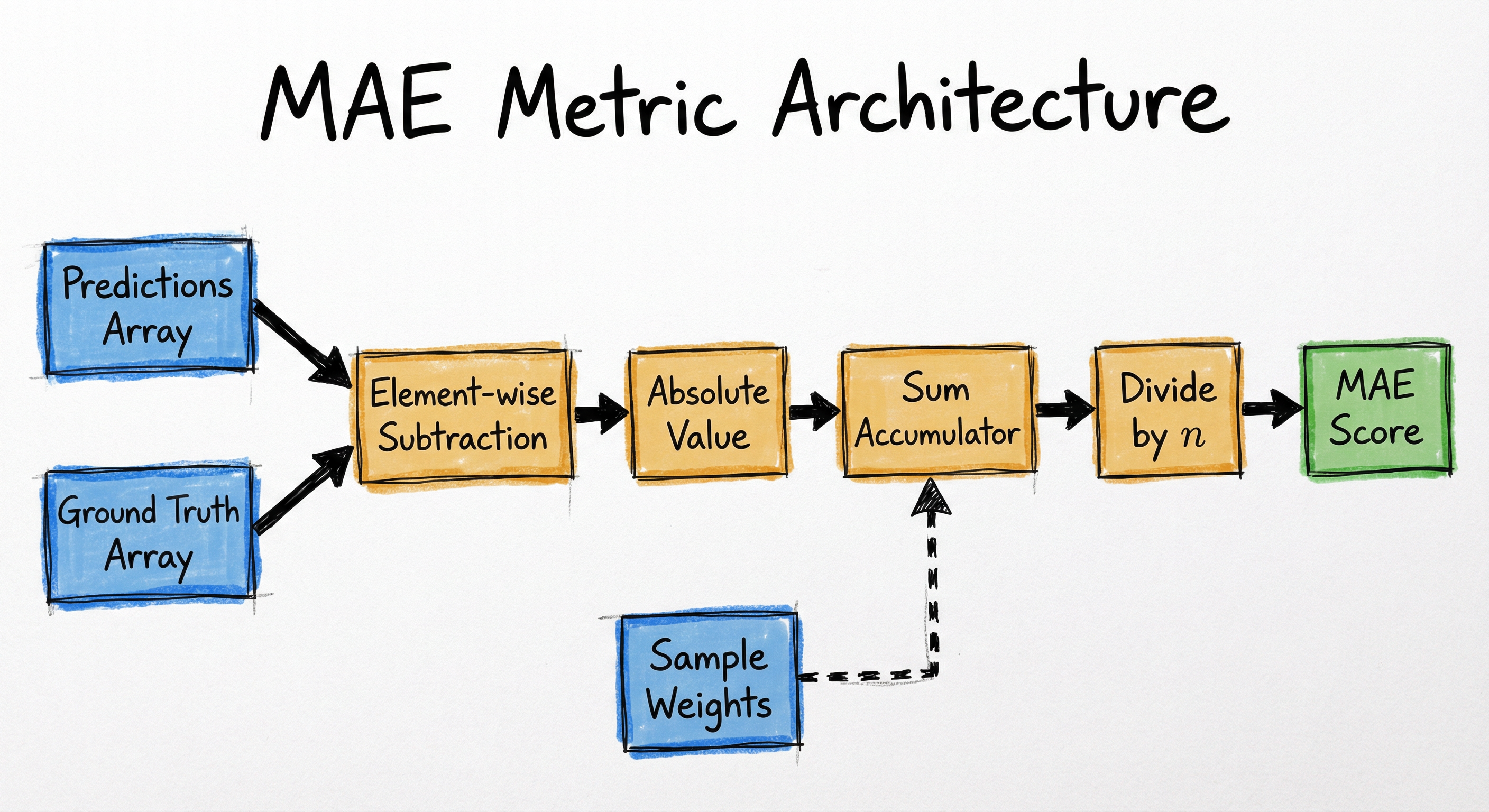
Internal Architecture

MAE computation follows a straightforward pipeline architecture that transforms paired predictions and ground truth values into a single scalar metric. The process involves element-wise operations followed by aggregation, making it highly parallelizable and suitable for both streaming and batch evaluation contexts.

MAE (Mean Absolute Error) in ML Systems Architecture — The architecture diagram shows a linear data flow from left to right. Predictions and ground trut...

The architecture supports both offline batch evaluation (computing MAE over a complete validation set) and online streaming evaluation (updating MAE incrementally as new predictions arrive). For production monitoring, a sliding window approach maintains MAE over recent predictions without storing all historical data.

Key Components

Input Validator

Ensures y_true and y_pred have matching shapes, checks for NaN/Inf values, validates numeric types, and optionally handles missing values based on configuration (skip, impute, or error).

Residual Computer

Performs element-wise subtraction $r_i = y_i - \hat{y}_i$ to compute raw residuals. This step preserves the sign of errors for potential diagnostic analysis before absolute value application.

Absolute Value Transformer

Applies $|r_i|$ to each residual, converting all errors to non-negative values. This is where MAE's symmetry property is enforced—both +5 and -5 errors become 5.

Aggregator

Sums all absolute errors: $\sum_{i=1}^{n} |r_i|$ . In weighted MAE variants, this component applies sample weights: $\sum_{i=1}^{n} w_i |r_i|$ . For streaming contexts, maintains running sum.

Normalizer

Divides the summed absolute errors by the count (or sum of weights) to produce the mean: $\text{MAE} = \frac{1}{n} \sum |r_i|$ . For percentage-based variants like MAPE, applies additional scaling.

Output Formatter

Returns MAE as a scalar float with appropriate precision. May include metadata like sample count, confidence intervals (via bootstrap), or breakdowns by data segments for monitoring dashboards.

Data Flow

Data flows linearly through the pipeline: input arrays enter the validator, pass through residual computation and absolute value transformation, get aggregated into a sum, normalized by sample count, and output as a scalar. For production systems, the architecture often includes parallel paths for computing multiple metrics simultaneously (MAE, RMSE, MAPE) to avoid redundant passes over the data. Checkpointing at the residual stage allows debugging by examining error distributions. In distributed settings (e.g., Spark, Dask), the subtraction and absolute value steps are mapped to workers, partial sums are shuffled to a reducer, and final division produces the global MAE.

The architecture diagram shows a linear data flow from left to right. Predictions and ground truth arrays merge at an element-wise subtraction step (orange), which produces residuals. These pass through an absolute value transformation (orange), then accumulate in a sum aggregator (blue), which optionally incorporates sample weights (dashed line from top). The sum is normalized by dividing by the count to produce the final MAE score (green). The pipeline emphasizes the sequential nature of operations and the optional weighting mechanism.

How to Implement

Implementing MAE in production ML systems involves more than just calling a library function—it requires careful consideration of numerical stability, edge cases, distributed computation, and integration with monitoring infrastructure. The most common approach uses established libraries like scikit-learn for offline evaluation and TensorFlow/PyTorch for training with MAE loss. However, custom implementations are often needed for streaming metrics, weighted variants, or integration with specific MLOps platforms.

Modern ML frameworks provide MAE in two contexts: as an evaluation metric (computed after predictions) and as a loss function (used during training). When used as a loss, MAE's non-differentiability at zero is handled via subgradient methods or smooth approximations. The choice between MAE and alternatives like Huber loss often depends on whether you want strict L1 behavior or a hybrid that's more optimization-friendly.

For large-scale systems, implementing MAE efficiently requires parallelization strategies. Since each sample's error can be computed independently, MAE is embarrassingly parallel across the residual computation and absolute value steps. Only the final sum requires coordination. This makes MAE well-suited for distributed evaluation frameworks like Apache Spark or Dask.

Basic MAE with Scikit-learn29 lines

from sklearn.metrics import mean_absolute_error
import numpy as np

# Ground truth and predictions
y_true = np.array([3.0, -0.5, 2.0, 7.0])
y_pred = np.array([2.5, 0.0, 2.0, 8.0])

# Compute MAE
mae = mean_absolute_error(y_true, y_pred)
print(f"MAE: {mae:.3f}")  # MAE: 0.500

# With sample weights (emphasize certain predictions)
sample_weight = np.array([1, 1, 1, 2])  # Last prediction weighted 2x
mae_weighted = mean_absolute_error(y_true, y_pred, sample_weight=sample_weight)
print(f"Weighted MAE: {mae_weighted:.3f}")  # MAE: 0.600

# Multi-output regression (multiple targets per sample)
y_true_multi = np.array([[0.5, 1], [-1, 1], [7, -6]])
y_pred_multi = np.array([[0, 2], [-1, 2], [8, -5]])

# Default: uniform average across outputs
mae_multi = mean_absolute_error(y_true_multi, y_pred_multi)
print(f"Multi-output MAE: {mae_multi:.3f}")  # MAE: 0.750

# Return MAE per output
mae_per_output = mean_absolute_error(
    y_true_multi, y_pred_multi, multioutput='raw_values'
)
print(f"Per-output MAE: {mae_per_output}")  # [0.5, 1.0]

This example demonstrates scikit-learn's mean_absolute_error function, which is the standard tool for offline evaluation. Key features: (1) handles 1D and multi-dimensional arrays, (2) supports sample weighting for imbalanced datasets or importance-based evaluation, (3) offers multioutput modes for multi-target regression. The function validates inputs, computes residuals, applies absolute value, and averages. For production pipelines, wrap this in a metric computation class that handles edge cases like empty arrays or all-zero predictions.

MAE Loss Function in TensorFlow/Keras46 lines

import tensorflow as tf
from tensorflow import keras
import numpy as np

# Build a simple regression model with MAE loss
model = keras.Sequential([
    keras.layers.Dense(64, activation='relu', input_shape=(10,)),
    keras.layers.Dense(32, activation='relu'),
    keras.layers.Dense(1)  # Single regression output
])

# Compile with MAE loss (also known as mean_absolute_error)
model.compile(
    optimizer='adam',
    loss='mae',  # Equivalent to keras.losses.MeanAbsoluteError()
    metrics=['mae', 'mse']  # Track both MAE and MSE during training
)

# Generate dummy training data
X_train = np.random.randn(1000, 10)
y_train = np.random.randn(1000, 1)

# Train with MAE loss
history = model.fit(
    X_train, y_train,
    validation_split=0.2,
    epochs=10,
    verbose=0
)

print(f"Final training MAE: {history.history['mae'][-1]:.3f}")
print(f"Final validation MAE: {history.history['val_mae'][-1]:.3f}")

# Using MAE as a standalone metric (not loss)
mae_metric = keras.metrics.MeanAbsoluteError()
y_true = tf.constant([[2.0], [4.0], [6.0]])
y_pred = tf.constant([[1.5], [4.2], [5.8]])

mae_metric.update_state(y_true, y_pred)
print(f"MAE metric: {mae_metric.result().numpy():.3f}")  # 0.233

# Reset and compute incrementally (useful for streaming)
mae_metric.reset_state()
for true, pred in zip(y_true, y_pred):
    mae_metric.update_state([true], [pred])
print(f"Incremental MAE: {mae_metric.result().numpy():.3f}")  # 0.233

This shows how to use MAE in TensorFlow/Keras for both training (as a loss function) and evaluation (as a metric). When used as a loss, Keras's automatic differentiation handles the non-differentiability at zero using subgradients. The MeanAbsoluteError metric class supports stateful computation, accumulating errors across batches—critical for large datasets that don't fit in memory. The .update_state() and .reset_state() pattern enables streaming evaluation where you process data in chunks and maintain running statistics. In production, you'd wrap this in a custom callback to log MAE to your monitoring system (MLflow, W&B, etc.) after each epoch or batch.

Custom MAE with Median Absolute Deviation (MedAE)89 lines

import numpy as np
from typing import Optional

def mean_absolute_error(
    y_true: np.ndarray,
    y_pred: np.ndarray,
    sample_weight: Optional[np.ndarray] = None,
    epsilon: float = 1e-10
) -> float:
    """
    Compute Mean Absolute Error with numerical stability.
    
    Args:
        y_true: Ground truth values, shape (n_samples,)
        y_pred: Predicted values, shape (n_samples,)
        sample_weight: Optional weights, shape (n_samples,)
        epsilon: Small value to prevent division by zero
    
    Returns:
        MAE as a scalar float
    """
    # Validate inputs
    y_true = np.asarray(y_true)
    y_pred = np.asarray(y_pred)
    
    if y_true.shape != y_pred.shape:
        raise ValueError(f"Shape mismatch: y_true {y_true.shape} vs y_pred {y_pred.shape}")
    
    # Compute residuals
    residuals = y_true - y_pred
    
    # Apply absolute value
    abs_errors = np.abs(residuals)
    
    # Apply sample weights if provided
    if sample_weight is not None:
        sample_weight = np.asarray(sample_weight)
        if sample_weight.shape != abs_errors.shape:
            raise ValueError("sample_weight must match y_true shape")
        weighted_errors = abs_errors * sample_weight
        mae = np.sum(weighted_errors) / (np.sum(sample_weight) + epsilon)
    else:
        mae = np.mean(abs_errors)
    
    return float(mae)

def median_absolute_error(
    y_true: np.ndarray,
    y_pred: np.ndarray
) -> float:
    """
    Compute Median Absolute Error (MedAE), even more robust to outliers.
    
    MedAE is the median of absolute errors, making it extremely robust.
    A single outlier affects MAE linearly, but MedAE is unaffected
    unless >50% of predictions are outliers.
    """
    residuals = np.asarray(y_true) - np.asarray(y_pred)
    abs_errors = np.abs(residuals)
    return float(np.median(abs_errors))

# Example with outliers
y_true = np.array([1.0, 2.0, 3.0, 4.0, 5.0])
y_pred_good = np.array([1.1, 2.1, 3.0, 3.9, 5.2])  # Small errors
y_pred_outlier = np.array([1.1, 2.1, 3.0, 3.9, 100.0])  # One huge outlier

mae_good = mean_absolute_error(y_true, y_pred_good)
mae_outlier = mean_absolute_error(y_true, y_pred_outlier)
medae_outlier = median_absolute_error(y_true, y_pred_outlier)

print(f"MAE (no outliers): {mae_good:.3f}")  # 0.140
print(f"MAE (with outlier): {mae_outlier:.3f}")  # 19.040 - heavily affected
print(f"MedAE (with outlier): {medae_outlier:.3f}")  # 0.100 - barely affected

# For production: return both MAE and MedAE to detect outlier influence
def robust_mae_report(y_true, y_pred):
    mae = mean_absolute_error(y_true, y_pred)
    medae = median_absolute_error(y_true, y_pred)
    ratio = mae / (medae + 1e-10)
    
    return {
        'mae': mae,
        'median_ae': medae,
        'mae_medae_ratio': ratio,  # >>1 indicates outlier influence
        'outlier_warning': ratio > 2.0
    }

report = robust_mae_report(y_true, y_pred_outlier)
print(f"\nRobust Report: {report}")

This example provides a production-ready custom implementation with three key features: (1) Input validation to catch shape mismatches early, (2) Numerical stability via epsilon in weighted division to prevent divide-by-zero, (3) Median Absolute Error (MedAE) as an ultra-robust companion metric. The robust_mae_report function is particularly valuable in production: it computes both MAE and MedAE, then calculates their ratio. If MAE >> MedAE (ratio > 2), you have outliers significantly skewing the mean—a critical signal for data quality monitoring. This pattern is used in systems like Swiggy's demand forecasting, where outlier detection prevents bad data from triggering false alerts.

Distributed MAE with Apache Spark60 lines

from pyspark.sql import SparkSession
from pyspark.ml.evaluation import RegressionEvaluator
from pyspark.ml.regression import LinearRegression
from pyspark.ml.feature import VectorAssembler

# Initialize Spark
spark = SparkSession.builder.appName("MAE_Evaluation").getOrCreate()

# Load predictions from a trained model (example with dummy data)
data = spark.createDataFrame([
    (1.0, 1.2),
    (2.0, 1.8),
    (3.0, 3.1),
    (4.0, 3.9),
    (5.0, 5.5)
], ["label", "prediction"])

# Method 1: Using RegressionEvaluator
evaluator = RegressionEvaluator(
    labelCol="label",
    predictionCol="prediction",
    metricName="mae"  # Other options: rmse, mse, r2
)

mae = evaluator.evaluate(data)
print(f"Spark MAE: {mae:.3f}")  # 0.240

# Method 2: Custom MAE using SQL aggregation (more flexible)
from pyspark.sql.functions import abs as spark_abs, avg

mae_custom = data.select(
    avg(spark_abs(data.label - data.prediction)).alias("mae")
).collect()[0]["mae"]

print(f"Custom MAE: {mae_custom:.3f}")  # 0.240

# Method 3: MAE per partition (for debugging distributed computation)
from pyspark.sql.functions import spark_partition_id, sum as spark_sum, count

partition_stats = data.select(
    spark_partition_id().alias("partition"),
    spark_abs(data.label - data.prediction).alias("abs_error")
).groupBy("partition").agg(
    spark_sum("abs_error").alias("sum_errors"),
    count("abs_error").alias("count")
).collect()

print("\nPer-partition MAE breakdown:")
total_sum = 0
total_count = 0
for row in partition_stats:
    partition_mae = row["sum_errors"] / row["count"]
    print(f"Partition {row['partition']}: MAE={partition_mae:.3f}, n={row['count']}")
    total_sum += row["sum_errors"]
    total_count += row["count"]

global_mae = total_sum / total_count
print(f"\nGlobal MAE (aggregated): {global_mae:.3f}")

spark.stop()

This demonstrates MAE computation in distributed settings using Apache Spark, essential for production ML systems processing billions of predictions. Spark's RegressionEvaluator provides built-in MAE, but the custom SQL approach (avg(abs(label - prediction))) offers more flexibility for weighted variants or conditional MAE (e.g., MAE by user segment). The per-partition breakdown is crucial for debugging: if one partition shows much higher MAE, you may have data skew or distribution issues. In practice, companies like Flipkart and Netflix use this pattern to evaluate recommendation and pricing models across massive datasets, computing MAE incrementally as predictions stream in from online serving systems.

Configuration Example43 lines

# Example configuration for MAE-based model monitoring in YAML
metrics:
  mae:
    enabled: true
    compute_interval: "1h"  # Recompute every hour
    aggregation_window: "24h"  # MAE over last 24 hours
    
    # Alerting thresholds
    thresholds:
      warning: 15.0    # MAE in target units
      critical: 25.0
      baseline: 10.5   # Historical baseline MAE
    
    # Compute MAE per data slice for fairness monitoring
    slices:
      - dimension: "user_segment"
        values: ["new_users", "power_users", "enterprise"]
      - dimension: "product_category"
        values: ["electronics", "fashion", "grocery"]
      - dimension: "region"
        values: ["north", "south", "east", "west"]
    
    # Companion metrics for context
    companion_metrics:
      - "median_absolute_error"  # Detect outlier influence
      - "mae_percentage"         # MAE / mean(y_true)
      - "p95_absolute_error"     # 95th percentile error
    
    # Data quality checks
    validation:
      min_samples: 100           # Require >=100 samples
      max_missing_ratio: 0.05    # Fail if >5% missing
      outlier_detection: "iqr"   # Flag outliers via IQR
    
    # Logging and storage
    logging:
      backend: "mlflow"
      tags:
        model_version: "v2.3"
        deployment: "production"
      artifacts:
        - "error_distribution_plot"
        - "mae_by_slice_table"

Common Implementation Mistakes

●
Not squaring before taking the root: Confusing MAE with RMSE. MAE is just mean(|errors|), not sqrt(mean(errors²)). Double-check you're using the right metric for your use case.
●
Ignoring scale differences: Comparing MAE across datasets with different target ranges is misleading. An MAE of 10 is excellent for predicting house prices (lakhs of rupees) but terrible for predicting product ratings (1-5 scale). Use MAPE (percentage) or normalize MAE by target range for cross-dataset comparisons.
●
Using MAE when you care about outliers: If large errors are catastrophic (e.g., predicting safe medication dosages), MAE's linear penalty is too lenient. Use RMSE or Huber loss to penalize outliers more heavily.
●
Division by zero with MAPE: Computing MAPE as mean(|y_true - y_pred| / y_true) fails when y_true = 0. Always check for zeros or use symmetric MAPE variants.
●
Forgetting to align time indices: In time series forecasting, ensure predictions and ground truth are aligned by timestamp. Shifted indices cause incorrect residuals and meaningless MAE.
●
Not monitoring MAE distribution: Reporting only the global MAE hides regional issues. Compute MAE by data slices (user cohorts, product categories, time windows) to detect fairness issues or data drift.
●
Misinterpreting MAE as worst-case error: MAE is an average—individual predictions can be much worse. Always report percentile-based metrics (P95, P99 errors) alongside MAE for production SLAs.
●
Using MAE for classification: MAE requires continuous targets. For class probabilities, use log loss or Brier score; for class labels, use accuracy or F1.

When Should You Use This?

Use When

You need stakeholder-friendly metrics: When reporting to non-technical teams (business, product, operations), MAE's interpretability ("predictions are off by X units on average") is invaluable.
Outliers are present but not catastrophic: For robust evaluation where occasional large errors shouldn't dominate the metric (e.g., delivery time prediction, demand forecasting).
Target variable is continuous and has a natural scale: MAE works best when the target has meaningful units (dollars, minutes, kilograms) rather than arbitrary scales.
You want to predict medians: If you train with MAE loss, your model learns to predict the conditional median—useful for skewed distributions where the median is more representative than the mean.
Symmetric error costs: When underestimating by 10 is equally bad as overestimating by 10, MAE's symmetry is appropriate.
Comparing models on the same target: MAE allows direct comparison when models predict the same variable (e.g., different forecasting approaches for the same demand signal).
Production monitoring dashboards: MAE is easy to plot, trend over time, and set thresholds for alerting ("alert if MAE > 20 minutes").

Avoid When

Large errors are unacceptable: For safety-critical or high-stakes applications (medical dosing, financial fraud), use RMSE or Huber loss to penalize outliers more heavily.
Comparing across different target scales: MAE of 100 for house prices vs. MAE of 2 for ratings aren't comparable. Use MAPE (percentage) or normalized metrics instead.
You need differentiability everywhere: MAE's non-differentiability at zero can complicate some optimization algorithms. Use MSE or Huber loss for smoother gradients.
Targets include zeros or very small values: MAPE (MAE's percentage cousin) explodes when dividing by near-zero ground truth. Stick to absolute MAE or use symmetric MAPE variants.
You care about directional bias: MAE treats +10 and -10 errors the same. If directional bias matters (e.g., always overpredicting inventory), track Mean Error (ME) separately.
Probabilistic forecasting: For uncertainty quantification or interval prediction, use quantile loss, CRPS (Continuous Ranked Probability Score), or likelihood-based metrics instead of point-estimate MAE.
Classification tasks: MAE is undefined for categorical targets. Use cross-entropy, accuracy, F1, or AUC-ROC for classification.

Key Tradeoffs

The central tradeoff in choosing MAE revolves around robustness vs. sensitivity:

MAE vs. MSE/RMSE: MAE is robust to outliers (linear penalty) but less sensitive to them, while MSE/RMSE heavily penalize large errors (quadratic penalty) but are skewed by outliers. This creates a philosophical choice: do you care about typical performance (MAE) or worst-case performance (RMSE)? In practice, report both: if RMSE >> MAE, you have outlier issues that MAE is hiding.

MAE vs. MAPE: MAE preserves units (interpretable) but is scale-dependent (hard to compare across datasets), while MAPE is scale-free (percentage) but fails near zero and can be skewed by small denominators. Use MAE for single-dataset evaluation, MAPE for cross-dataset or cross-product comparisons.

MAE vs. Huber Loss: MAE is simpler and fully linear, while Huber loss combines MAE's robustness (linear for large errors) with MSE's smoothness (quadratic for small errors). Huber requires tuning a threshold parameter δ but offers better optimization properties. For training, Huber often wins; for evaluation, MAE's simplicity is preferred.

Mean vs. Median forecasting: Minimizing MAE during training yields median predictions, while minimizing MSE yields mean predictions. For skewed distributions (income, housing prices, demand spikes), medians are often more robust and actionable. However, medians don't aggregate nicely: the median of group A + group B ≠ median(A) + median(B), complicating hierarchical forecasting.

Metric	Outlier Sensitivity	Interpretability	Differentiability	Median/Mean Target
MAE	Low (linear)	High (same units)	No (at zero)	Median
MSE	High (quadratic)	Low (squared units)	Yes (everywhere)	Mean
RMSE	High (quadratic)	Medium (same units)	Yes (mostly)	Mean
MAPE	Low (linear)	High (percentage)	No (at zero)	Median (of %)
Huber	Tunable (hybrid)	Medium	Yes (everywhere)	Tunable

In production systems, the best practice is to compute multiple metrics and understand their relationships. If MAE = 10 and RMSE = 30, you know large errors are present. If MAE ≈ MedAE, your error distribution is symmetric without heavy outliers.

Alternatives & Comparisons

MSE/RMSE

MSE (Mean Squared Error) and RMSE (Root Mean Squared Error) penalize large errors quadratically, making them more sensitive to outliers than MAE. Use RMSE when large errors are particularly costly (e.g., safety-critical systems, financial forecasting) and when you want to optimize for the mean rather than the median. RMSE also has nice mathematical properties (differentiable everywhere) that simplify optimization. Choose MAE for robustness and interpretability; choose RMSE for outlier sensitivity and smooth gradients.

R² Score

R² (coefficient of determination) measures the proportion of variance explained by the model, ranging from -∞ to 1. Unlike MAE (absolute error), R² is scale-free and indicates relative improvement over a baseline (mean predictor). Use R² when you want to know "how much better is my model than just predicting the mean?" rather than "how far off are my predictions?" R² is great for model selection but less actionable for production monitoring—stakeholders understand "predictions are off by 10 minutes (MAE)" better than "R² = 0.85."

MAPE

MAPE (Mean Absolute Percentage Error) is MAE expressed as a percentage: mean(|y_true - y_pred| / y_true) × 100%. MAPE is scale-free, making it ideal for comparing forecasts across products or datasets with different units. However, MAPE fails when ground truth contains zeros (division by zero) and is asymmetric (over-predictions penalized less than under-predictions). Use MAPE for cross-product comparisons or when stakeholders prefer percentages; use MAE when targets can be zero or near-zero, or when you need symmetric error treatment.

Residual Plot

Residual plots visualize prediction errors (y_true - y_pred) against predicted values or input features. Unlike MAE (a single scalar), residual plots reveal patterns in errors: heteroscedasticity (variance changes with predictions), bias (systematic over/under-prediction), or non-linearity (missed patterns). Use MAE for quantifying overall accuracy; use residual plots for diagnosing model deficiencies and understanding where errors concentrate. They're complementary: MAE answers "how accurate?", residual plots answer "where and why are we wrong?"

Pros, Cons & Tradeoffs

Advantages

Highly interpretable: MAE is expressed in the same units as the target variable, making it easy to communicate to non-technical stakeholders. "Predictions are off by 8 minutes on average" is immediately actionable.
Robust to outliers: Unlike MSE/RMSE, MAE's linear penalty doesn't let a few large errors dominate the metric, providing a more representative view of typical model performance.
Symmetric treatment of errors: Over-predictions and under-predictions contribute equally to MAE, which is appropriate when both directions of error have similar costs.
Mathematically simple: No squaring or square roots—just absolute values and averaging. This simplicity makes MAE fast to compute and easy to implement in any language or distributed framework.
Suitable for skewed distributions: Training with MAE loss yields models that predict the conditional median, which is often more robust and meaningful than the mean for skewed targets (income, housing prices, demand spikes).
Easy to monitor over time: MAE's stability and interpretability make it ideal for time-series dashboards, alerting systems, and SLA tracking in production ML systems.
Parallelizable: Computing MAE is embarrassingly parallel (each sample's error is independent), making it efficient for large-scale batch and streaming evaluation.

Disadvantages

Scale-dependent: MAE values aren't comparable across datasets or targets with different scales. An MAE of 100 is meaningless without knowing whether you're predicting rupees, kilograms, or seconds.
Underemphasizes large errors: The linear penalty means a prediction off by 100 contributes only 10× more than one off by 10, whereas in some domains (medical, financial), large errors should be penalized exponentially.
Non-differentiable at zero: The absolute value function has undefined derivative at zero, complicating gradient-based optimization. While subgradient methods handle this, smoother losses (MSE, Huber) converge faster in some cases.
Doesn't capture error variance: MAE is a point estimate of central tendency; it doesn't tell you about the spread of errors. Two models with the same MAE can have very different error distributions (one consistent, one with high variance).
Insensitive to directional bias: MAE treats systematic over-prediction and under-prediction the same. If your model always overestimates by 5%, MAE won't highlight this bias—track Mean Error (ME) or signed residuals separately.
Not suitable for probabilistic forecasting: MAE evaluates point predictions only; it doesn't assess the quality of prediction intervals, quantiles, or full predictive distributions. Use quantile loss or CRPS for uncertainty quantification.
Can hide data quality issues: MAE's robustness is a double-edged sword—it might not alert you to outliers or data corruption that RMSE would catch. Always pair MAE with outlier detection and MedAE for comprehensive monitoring.

Placement in an ML System

MAE sits at the evaluation and monitoring stage of ML pipelines, serving dual roles: (1) offline evaluation during model development and selection, and (2) online monitoring in production systems. In the offline context, MAE is computed on validation/test sets to compare models, tune hyperparameters, and decide when to retrain. It typically appears in experiment tracking systems (MLflow, W&B) alongside other metrics like RMSE and R².

In production, MAE becomes a critical operational metric. Predictions flow from inference endpoints to ground truth collectors (often via event streams like Kafka), and MAE is computed in near-real-time over sliding windows (hourly, daily). This streaming MAE feeds into monitoring dashboards, alerting systems, and automated retraining triggers. For example, Swiggy's demand forecasting system continuously tracks MAE across product categories; if MAE spikes above thresholds, alerts notify on-call engineers and may trigger automatic fallback to simpler baseline models.

MAE also interfaces with A/B testing frameworks: when comparing model variants (A vs. B), MAE provides a clear business metric for declaring winners. Unlike proxy metrics, MAE directly measures prediction accuracy, making it suitable for automated decision-making in multi-armed bandit or contextual bandit setups. Downstream systems like model registries store MAE metadata with each model version, enabling lineage tracking and regression detection ("new model has 20% higher MAE than previous version—investigate before promotion").

Pipeline Stage

Evaluation & Monitoring

Upstream

model-inference
batch-prediction
online-prediction

Downstream

model-registry
monitoring-dashboard
alerting-system
ab-testing-framework

Scaling Bottlenecks

MAE computation scales linearly with sample count and is embarrassingly parallel, so bottlenecks are rare. For streaming evaluation over millions of predictions per second, maintain running sums in memory (numerator: sum of absolute errors, denominator: count) and periodically compute MAE = sum / count. For distributed batch jobs (Spark, Dask), ensure residual computation happens locally on workers, with only final aggregation requiring network communication. Watch for memory issues when storing raw errors for percentile calculations—use reservoir sampling or t-digest for approximate percentiles in constant memory. If computing MAE per slice (e.g., per user segment), cardinality explosion can occur; use sketching algorithms or limit to top-K slices.

Production Case Studies

SwiggyFood Delivery & Quick Commerce

Swiggy Instamart faced challenges with traditional forecasting metrics not aligning with operational objectives. They implemented an adaptive metric alignment system that uses MAE alongside other metrics to balance demand prediction accuracy across diverse product categories. The system computes MAE per product family, recognizing that a 10-unit error for high-volume items (e.g., milk) has different operational impact than for niche products (e.g., specialty spices). They enhanced MAE with segment-specific thresholds and combined it with bias metrics to prevent systematic over/under-stocking.

Outcome:

Improved demand forecasting accuracy by aligning ML metrics (including MAE) with business objectives like minimizing stockouts and waste. The adaptive approach reduced operational friction and enabled better inventory planning across thousands of SKUs in quick commerce operations.

UberRide-Hailing & Logistics

Uber's DeepETA system uses deep learning for global ETA prediction, with Mean Absolute Error (MAE) as the primary metric to measure accuracy improvements over the incumbent XGBoost model across different segments (delivery vs rides, long vs short trips).

Outcome:

DeepETA improves MAE significantly over the baseline XGBoost model through segment-specific bias adjustment layers. The system serves billions of ETA predictions daily with low latency while maintaining high accuracy across Uber's global operations.

NetflixStreaming Media

Netflix uses MAE for evaluating QoE (Quality of Experience) prediction models, which forecast metrics like buffering time, startup latency, and video quality. MAE's robustness to outliers is crucial because streaming performance has heavy-tailed distributions—most streams are smooth, but a few have catastrophic issues (network outages, CDN failures). Netflix computes MAE for predicted vs. actual streaming quality metrics, using it to compare algorithmic improvements (e.g., new adaptive bitrate algorithms). They pair MAE with percentile-based metrics (P95, P99) to ensure tail performance meets SLAs.

Outcome:

MAE provides a stable baseline metric for A/B testing video quality improvements. Its interpretability ("predicted buffering time is off by 2 seconds on average") facilitates decision-making in cross-functional teams, while its robustness prevents outlier network events from skewing metric comparisons.

AirbnbHospitality & Marketplace

Airbnb built a machine learning model to predict the booking value of homes listed on their platform. MAE was chosen as a primary evaluation metric because stakeholders (hosts and pricing teams) needed to understand prediction accuracy in monetary terms (USD). The model predicts nightly booking value, and MAE directly answers: "On average, how far off are our price predictions?" Airbnb compared MAE across different listing types (entire homes, private rooms, shared spaces) and geographies to identify where the model performed well and where it needed refinement. They also tracked MAE over time to detect concept drift as market conditions changed.

Outcome:

MAE enabled Airbnb to communicate model performance to non-technical stakeholders (hosts) and set realistic expectations for pricing suggestions. The metric guided feature engineering efforts by highlighting which listing attributes (location, amenities, seasonality) most reduced prediction error.

FlipkartE-Commerce

Flipkart uses MAE for demand forecasting models that predict product sales across millions of SKUs during normal periods and high-traffic events like Big Billion Days. MAE provides a product-agnostic metric for comparing forecasts across diverse categories (electronics, fashion, groceries) when normalized by average sales. Flipkart computes MAE at multiple granularities: SKU-level, category-level, and warehouse-level, enabling targeted improvements. They combine MAE with bias metrics to prevent systematic over-forecasting (leading to excess inventory) or under-forecasting (causing stockouts).

Outcome:

MAE-driven demand forecasting reduced inventory holding costs and stockout rates. The interpretability of MAE ("forecast is off by X units on average") facilitated collaboration between data science and supply chain teams, enabling joint optimization of ML models and logistics operations.

Tooling & Ecosystem

Scikit-learn

PythonOpen Source

Provides sklearn.metrics.mean_absolute_error() for computing MAE on NumPy arrays or Pandas DataFrames. Supports sample weights for imbalanced datasets and multi-output regression. The standard tool for offline model evaluation in Python.

TensorFlow/Keras

PythonOpen Source

Offers tf.keras.losses.MeanAbsoluteError as a loss function for training neural networks and tf.keras.metrics.MeanAbsoluteError as a stateful metric for evaluation. Supports batch-wise and streaming computation, essential for large-scale deep learning workflows.

PyTorch

PythonOpen Source

Provides torch.nn.L1Loss (equivalent to MAE) for training and torch.nn.functional.l1_loss for functional API. Fully integrates with PyTorch's autograd for gradient-based optimization with MAE loss.

Apache Spark MLlib

Scala/PythonOpen Source

Distributed evaluation via pyspark.ml.evaluation.RegressionEvaluator with metricName='mae'. Computes MAE over massive datasets in parallel across Spark clusters, essential for big data ML pipelines.

MLflow

PythonOpen Source

Experiment tracking platform that logs MAE (and other metrics) during model training. Provides UI for comparing MAE across model versions, hyperparameter settings, and datasets. Integrates with scikit-learn, TensorFlow, PyTorch for automatic metric logging.

Weights & Biases (W&B)

PythonCommercial

ML experiment tracking and visualization platform. Automatically logs MAE from scikit-learn, Keras, PyTorch models. Provides interactive dashboards for plotting MAE over training epochs, comparing across experiments, and detecting overfitting via train vs. validation MAE divergence.

Evidently AI

PythonOpen Source

ML monitoring and observability tool that tracks MAE in production. Generates drift reports comparing MAE distributions over time, detects when MAE degrades beyond thresholds, and provides visualizations for error analysis. Supports integration with monitoring stacks (Prometheus, Grafana).

Amazon SageMaker

PythonCommercial

AWS's managed ML platform automatically computes MAE for regression models via Model Monitor. Tracks MAE in production, sets up CloudWatch alarms on MAE thresholds, and triggers retraining workflows when MAE degrades. Integrates with SageMaker Pipelines for end-to-end MLOps.

Research & References

Beyond RMSE and MAE: Introducing EAUC to unmask hidden bias and unfairness in dyadic regression models

Rodrigo Alves, Célia Talma, Ludovic dos Santos, et al. (2025)arXiv preprint (v4, May 2025)

This paper shows that global error metrics like MAE and RMSE are insufficient to capture eccentricity bias—systematic errors favoring popular items or majority groups. The authors introduce EAUC (Eccentricity-Area Under the Curve) as a complementary metric that measures how error rates vary across the popularity spectrum. Critical insight: MAE might look acceptable globally while hiding unfairness toward niche users or items.

Machine Learning Evaluation Metric Discrepancies across Programming Languages and Their Components: Need for Standardization

H. R. Arabnia, et al. (2025)arXiv preprint (March 2025)

Examines implementation consistency of metrics like MAE, MSE, RMSE across Python (scikit-learn, TensorFlow, PyTorch), R, and Julia. Found MAE implementations are highly consistent across languages, unlike precision/recall metrics in classification. Advocates for standardized metric definitions to prevent evaluation discrepancies when comparing models implemented in different frameworks.

A Comprehensive Survey of Regression Based Loss Functions for Time Series Forecasting

Aryan Jadon, Avinash Patil, Shruti Jadon (2022)arXiv preprint

Comprehensive review of loss functions for time series forecasting, including MAE, MSE, Huber, quantile loss, and MAPE. Highlights MAE's connection to median forecasting and its suitability for skewed distributions. Discusses how MAE relates to quantile loss (MAE is the special case at q=0.5) and provides guidance on choosing loss functions based on distribution characteristics.

Interview & Evaluation Perspective

Common Interview Questions

●
When would you choose MAE over RMSE for evaluating a regression model?
●
Explain how MAE handles outliers differently from MSE.
●
What does it mean that minimizing MAE during training yields median predictions?
●
How would you implement MAE in a distributed system like Spark?
●
What are the limitations of using MAE for comparing models across different datasets?
●
How would you monitor MAE in a production ML system?

Key Points to Mention

●
Interpretability: MAE is in the same units as the target, making it easy to explain to stakeholders ("predictions are off by X units on average").
●
Robustness to outliers: MAE's linear penalty prevents large errors from dominating the metric, unlike RMSE's quadratic penalty.
●
Median vs. mean forecasting: Training with MAE loss optimizes for the conditional median, while MSE optimizes for the conditional mean—important for skewed distributions.
●
Non-differentiability: Mention that MAE's absolute value is non-differentiable at zero, requiring subgradient methods or smooth approximations (Huber loss) for optimization.
●
Scale dependency: Emphasize that MAE comparisons are only valid within the same target scale; use MAPE or normalized MAE for cross-dataset comparisons.
●
Complementary metrics: In practice, report MAE alongside MedAE, RMSE, and percentile errors to capture both typical and tail behavior.
●
Production monitoring: Discuss slice-based MAE (per user segment, product category) to detect fairness issues and data drift.
●
Connection to L1 regularization: MAE is L1 loss for prediction error, related to L1 regularization (Lasso) which promotes sparsity.

Pitfalls to Avoid

●
Confusing MAE with RMSE or forgetting to take the absolute value before averaging.
●
Claiming MAE is always better than RMSE—each has appropriate use cases depending on whether you care about typical vs. worst-case errors.
●
Ignoring that MAE doesn't capture directional bias (systematic over/under-prediction)—always mention tracking Mean Error (ME) separately.
●
Forgetting edge cases: division by zero in weighted MAE, shape mismatches, handling NaNs in production data.
●
Not discussing the interpretation gap when comparing MAE across different scales or domains.
●
Overlooking that MAE's robustness can hide data quality issues—pair with outlier detection and MedAE.

Senior-Level Expectation

Senior/staff-level candidates should go beyond basic MAE mechanics and demonstrate systems thinking. Discuss how MAE fits into the broader ML lifecycle: choosing MAE vs. RMSE based on business context (e.g., symmetric vs. asymmetric error costs), implementing slice-based MAE for fairness monitoring, designing streaming MAE computation for production monitoring with bounded memory, and integrating MAE into automated retraining triggers. Mention real-world tradeoffs: MAE's interpretability vs. RMSE's sensitivity to outliers, the challenge of setting MAE thresholds for alerting (what's "good enough"?), and the need for multi-metric evaluation (MAE + MedAE + P95 error) to capture the full picture. Bonus points for discussing adaptive metric alignment (as seen in Swiggy's case study) where MAE is weighted or normalized by business impact. Demonstrate awareness of research trends: eccentricity bias (EAUC paper), metric standardization across frameworks, and the connection between MAE and quantile regression.

Summary

Mean Absolute Error (MAE) stands as one of the most intuitive and widely adopted metrics for regression evaluation, offering a perfect balance between mathematical simplicity and practical interpretability. By measuring the average magnitude of prediction errors using absolute values, MAE provides stakeholders with a clear, actionable understanding of model performance: "On average, predictions are off by X units." This interpretability, combined with robustness to outliers and symmetric treatment of errors, makes MAE indispensable in production ML systems—from Swiggy's demand forecasting to Uber's ETA prediction and Netflix's QoE modeling.

MAE's key strength lies in its linearity: errors contribute proportionally without the quadratic amplification of MSE/RMSE, making it resistant to outlier contamination and representative of typical model behavior. This property connects MAE to median forecasting—models trained with MAE loss predict conditional medians rather than means, which is particularly valuable for skewed distributions common in real-world applications (income, housing prices, demand spikes). However, this robustness is a double-edged sword: MAE might hide catastrophic errors in tail cases or mask data quality issues that RMSE would expose. Best practice involves reporting MAE alongside complementary metrics (MedAE for ultra-robustness, RMSE for outlier sensitivity, percentile errors for tail behavior) to capture the full picture of model performance.

In the ML system lifecycle, MAE serves dual roles: as an offline evaluation metric for model selection and hyperparameter tuning, and as a production monitoring signal for detecting performance degradation and data drift. Modern ML platforms (MLflow, W&B, SageMaker) track MAE across experiments, while monitoring systems (Evidently AI, Prometheus) alert on MAE threshold breaches. The metric's simplicity enables efficient computation even in distributed settings (Spark, Dask), where embarrassingly parallel residual computation scales linearly with data size. For streaming scenarios, running statistics (sum of errors, count) enable constant-memory MAE updates, critical for real-time monitoring in high-throughput systems.

Successful deployment of MAE requires understanding its limitations and context-dependencies. MAE is scale-dependent—comparing across datasets demands normalization (MAPE, percentage-of-mean, or relative MAE). MAE is symmetric—directional bias (systematic over/under-prediction) requires tracking Mean Error separately. MAE averages globally—segment-specific MAE reveals fairness issues and heterogeneous performance. And MAE optimizes for typical cases—business metrics may demand weighted variants or quantile loss to handle asymmetric costs. The research frontier (EAUC for eccentricity bias, metric standardization across frameworks, integration with probabilistic forecasting) continues to expand MAE's capabilities, ensuring its relevance in evolving ML systems. Whether you're forecasting delivery times, predicting product prices, or estimating demand, MAE provides a solid foundation for evaluation—just remember to pair it with domain knowledge, business context, and complementary metrics for holistic model assessment.

Concept Snapshot

Why This Concept Exists

Core Intuition & Mental Model

Technical Foundations

Internal Architecture

Key Components

Data Flow

How to Implement

Common Implementation Mistakes

When Should You Use This?

Use When

Avoid When

Key Tradeoffs

Alternatives & Comparisons

Pros, Cons & Tradeoffs

Advantages

Disadvantages

Placement in an ML System

Pipeline Stage

Upstream

Downstream

Scaling Bottlenecks

Production Case Studies

Tooling & Ecosystem

Research & References

Interview & Evaluation Perspective

Common Interview Questions

Key Points to Mention

Pitfalls to Avoid

Senior-Level Expectation

Summary

Related Blocks & Further Reading

Related ML Blocks

Further Reading