Uplift Model in Machine Learning
Uplift modeling is one of the most underappreciated yet high-impact techniques in applied machine learning. While most ML practitioners are comfortable building models that predict who will convert, uplift modeling asks the far more valuable question: who will convert because of our intervention? The distinction is subtle but enormously consequential -- it is the difference between targeting people who were going to buy anyway and targeting people whose behavior you can actually change.
At its core, uplift modeling estimates the Conditional Average Treatment Effect (CATE) -- the incremental causal impact of a treatment (a coupon, an ad, a notification, a drug) on an individual's outcome, conditioned on their features. This moves us from correlation-based targeting ("users who look like buyers") to causation-based targeting ("users whose buying behavior is caused by our action"). The practical result? Instead of spending your marketing budget on customers who would have purchased regardless, you spend it on the persuadables -- those who only convert when treated.
The field has matured rapidly since its early days in direct marketing at companies like Stochastic Solutions in the mid-2000s. Today, uplift modeling is used at Uber for rider and driver promotions, at Booking.com for personalized discount allocation, at Wayfair for display remarketing, and increasingly at Indian companies like Swiggy and Flipkart for coupon targeting and retention campaigns. Meta-learner frameworks (S-learner, T-learner, X-learner, R-learner) provide flexible approaches that can wrap around any supervised learning algorithm, while specialized tools like CausalML, scikit-uplift, and EconML make implementation accessible.
Evaluation is where uplift modeling gets tricky -- you can never observe both the treated and untreated outcomes for the same individual (the fundamental problem of causal inference). Instead, practitioners rely on the Qini curve, uplift curve, and their area-based summaries (AUUC, Qini coefficient) to assess model quality. These metrics measure whether your model successfully ranks individuals by their true treatment effect, enabling you to allocate scarce resources to those who benefit most.
If you are building any system that involves deciding whom to treat -- whether that is sending a push notification, offering a discount, assigning a medical therapy, or showing an ad -- uplift modeling should be in your toolkit. This guide covers everything from the mathematical foundations to production deployment patterns, with real code examples and industry case studies.
Concept Snapshot
- What It Is
- A causal machine learning technique that estimates the incremental effect of a treatment on an individual's outcome (CATE), enabling targeted interventions on those most likely to be positively influenced.
- Category
- Evaluation / Experimentation
- Complexity
- Advanced
- Inputs / Outputs
- Inputs: features X, treatment assignment T (binary or multi-valued), outcome Y, and optionally propensity scores. Outputs: individual-level treatment effect estimates (uplift scores) that rank individuals by predicted causal impact.
- System Placement
- Sits after A/B test data collection and before targeting/allocation decisions. In the ML pipeline, it operates in the evaluation and decision-optimization stage, consuming experimental data and producing targeting policies.
- Also Known As
- Incremental modeling, True lift modeling, Differential response modeling, Net modeling, Heterogeneous treatment effect estimation, Individual treatment effect (ITE) estimation
- Typical Users
- Data Scientists, ML Engineers, Growth/Marketing Analysts, Causal Inference Researchers, Product Managers (Growth teams), Health Economists
- Prerequisites
- A/B testing and randomized controlled trials, Binary classification and regression, Potential outcomes framework (Rubin causal model), Propensity scores and confounding, Supervised learning fundamentals
- Key Terms
- CATE (Conditional Average Treatment Effect)ITE (Individual Treatment Effect)ATE (Average Treatment Effect)S-learner / T-learner / X-learner / R-learnerQini curve / Qini coefficientAUUC (Area Under Uplift Curve)Persuadables / Sure Things / Lost Causes / Do Not DisturbFundamental problem of causal inferencePropensity scoreCounterfactual
Why This Concept Exists
The Targeting Problem No Response Model Can Solve
Consider a common scenario at an Indian e-commerce platform like Flipkart or Myntra. You have a budget for 1 million promotional discount coupons, but your customer base is 50 million. A traditional response model predicts P(purchase | features) and ranks customers by predicted purchase probability. The top 1 million get the coupon.
But here is the critical flaw: the customers most likely to purchase are often the ones who would have purchased anyway, coupon or not. These are your loyal, high-frequency buyers. By targeting them, you are giving away margin on sales that would have happened organically. Meanwhile, there is a segment of customers who only purchase when nudged with a discount -- the persuadables -- and they might rank lower on a simple response model because their baseline purchase probability is modest.
Uplift modeling solves this by estimating not P(purchase), but P(purchase | treated) - P(purchase | not treated) -- the incremental effect of the coupon on each individual. This is the CATE.
The Four Customer Segments
Uplift modeling implicitly segments your customer base into four groups, a taxonomy first articulated by Radcliffe (2007):
- Sure Things: Will convert whether treated or not. Treatment has zero effect. Targeting them wastes budget.
- Persuadables: Will convert only if treated. Treatment has a large positive effect. These are your target audience.
- Lost Causes: Will not convert regardless of treatment. Zero effect. Targeting them also wastes budget.
- Do Not Disturb (Sleeping Dogs): Will actually be harmed by treatment -- they would have converted, but the treatment annoys them into not converting (negative treatment effect). Targeting them actively destroys value.
Traditional response models conflate Sure Things with Persuadables (both have high P(purchase | treated)). Only uplift modeling distinguishes between them by estimating the causal effect.
Historical Context
The concept of differential response modeling dates back to the late 1990s, when Nicholas Radcliffe at Stochastic Solutions developed the first commercial uplift modeling tools for direct mail campaigns in the UK. His 1999 paper introduced differential response analysis -- modeling the change in behavior caused by a specific action rather than predicting behavior itself.
The field gained academic rigor through two parallel streams: (1) the causal inference community (Rubin, Athey, Imbens) developing methods for heterogeneous treatment effect estimation, and (2) the marketing analytics community (Radcliffe, Lo, Gutierrez, Gerardy) developing practical uplift algorithms. These streams converged around 2017-2019 with Kunzel et al.'s influential metalearners paper and Uber's open-source CausalML library, which brought uplift modeling to mainstream ML engineering.
Today, uplift modeling is a core capability at companies allocating scarce resources: promotions, ad impressions, clinical treatments, customer service interventions, and product feature rollouts.
Key Insight: Uplift modeling exists because optimizing who to treat requires estimating causal effects, not just predictions. The shift from "who will respond" to "who will respond because of us" is the conceptual leap that separates correlation-based targeting from causal targeting.
Core Intuition & Mental Model
The Doctor's Dilemma Analogy
Imagine you are a doctor with 100 patients and only 30 doses of an expensive medicine (say, ₹50,000 per dose). A standard predictive model tells you which patients are most likely to recover. But some of those patients would recover on their own -- they are healthy enough that they do not need the medicine. Others are so sick that even the medicine cannot help. The patients you should prioritize are those who will recover only if given the medicine but will remain sick without it.
Uplift modeling is the method for identifying exactly those patients. Instead of predicting P(recovery), you estimate P(recovery | medicine) - P(recovery | no medicine) for each patient. The patients with the highest positive difference -- the persuadables in marketing language, or responders in clinical language -- get the medicine.
The Two Worlds You Cannot Both Observe
Here is the fundamental challenge: for any given individual, you can only observe one reality. Either they received the treatment (the coupon, the medicine, the ad) and you see what happened, or they did not receive it and you see what happened. You can never observe both outcomes for the same person at the same time. This is the fundamental problem of causal inference -- you are always missing one counterfactual.
Uplift modeling cleverly works around this by using groups of similar individuals. In a randomized A/B test, some people are randomly assigned to treatment and others to control. Within any subgroup of similar individuals (defined by their features), the difference in average outcomes between treated and control groups estimates the CATE for that subgroup. Meta-learners formalize different strategies for combining these group-level signals into individual-level uplift predictions.
Why "Just Subtract Two Models" Is Not Enough
A naive approach is the two-model (T-learner) method: build one model on treated data to predict P(Y=1 | X, T=1) and another on control data to predict P(Y=1 | X, T=0), then subtract. This works sometimes, but it has a critical flaw: each model is optimized to predict the outcome, not the treatment effect. Small errors in each model compound into large errors in the difference. If Model A predicts 0.42 and Model B predicts 0.40, the estimated uplift of 0.02 might be entirely noise.
More sophisticated approaches like the X-learner and R-learner directly target the treatment effect during optimization, leading to more precise estimates -- especially when treatment effects are small relative to outcome variance, which is the norm in most real-world applications. Understanding why these improvements matter is what separates practitioners who deploy working uplift systems from those who get disappointing results.
Mental Model: Think of uplift modeling as building a differential signal detector. You are not measuring the signal (outcome) itself -- you are measuring the tiny change in signal caused by a specific intervention, in the presence of much louder baseline noise.
Technical Foundations
Potential Outcomes Framework
We adopt the Rubin causal model (Neyman-Rubin framework). For each individual with features , define two potential outcomes:
- : outcome if individual receives treatment
- : outcome if individual receives control
The Individual Treatment Effect (ITE) is:
The fundamental problem of causal inference is that we only observe one of or , never both. The observed outcome is:
where is the treatment assignment.
CATE: The Estimand of Interest
The Conditional Average Treatment Effect (CATE) is the expected ITE conditional on features:
This is the target quantity that uplift models estimate. The Average Treatment Effect (ATE) is its unconditional version:
Identifying Assumptions
CATE is identifiable from observational data under:
- Unconfoundedness (Ignorability): -- treatment assignment is independent of potential outcomes given features. Automatically satisfied in randomized experiments.
- Overlap (Positivity): for all -- every individual has a non-zero chance of being in either group.
- SUTVA (Stable Unit Treatment Value Assumption): No interference between individuals; one individual's treatment does not affect another's outcome.
Meta-Learner Formulations
S-Learner (Single Model): Fit a single model on . Estimate CATE as:
T-Learner (Two Models): Fit separate models on treatment and control groups: on and on . Estimate:
X-Learner (Kunzel et al., 2019): Three-stage procedure:
- Fit and as in T-learner.
- Compute imputed treatment effects: for treated, for control.
- Fit models on and on . Combine: where is the propensity score.
R-Learner (Robinson decomposition): Minimize a loss that directly targets treatment effect: where and .
Evaluation Metrics
Qini Coefficient: The area between the model's Qini curve and the random targeting line. The Qini curve plots cumulative incremental conversions as a function of the fraction of population targeted (sorted by predicted uplift, highest first): where and are the number of conversions in treatment and control within the top fraction, and are total treatment and control sizes.
AUUC (Area Under Uplift Curve): Similar to Qini but plots the uplift (difference in conversion rates) as a function of fraction targeted:
Note: Neither AUUC nor Qini coefficient is normalized -- their best possible values depend on the data. Always compare against random targeting and perfect targeting baselines.
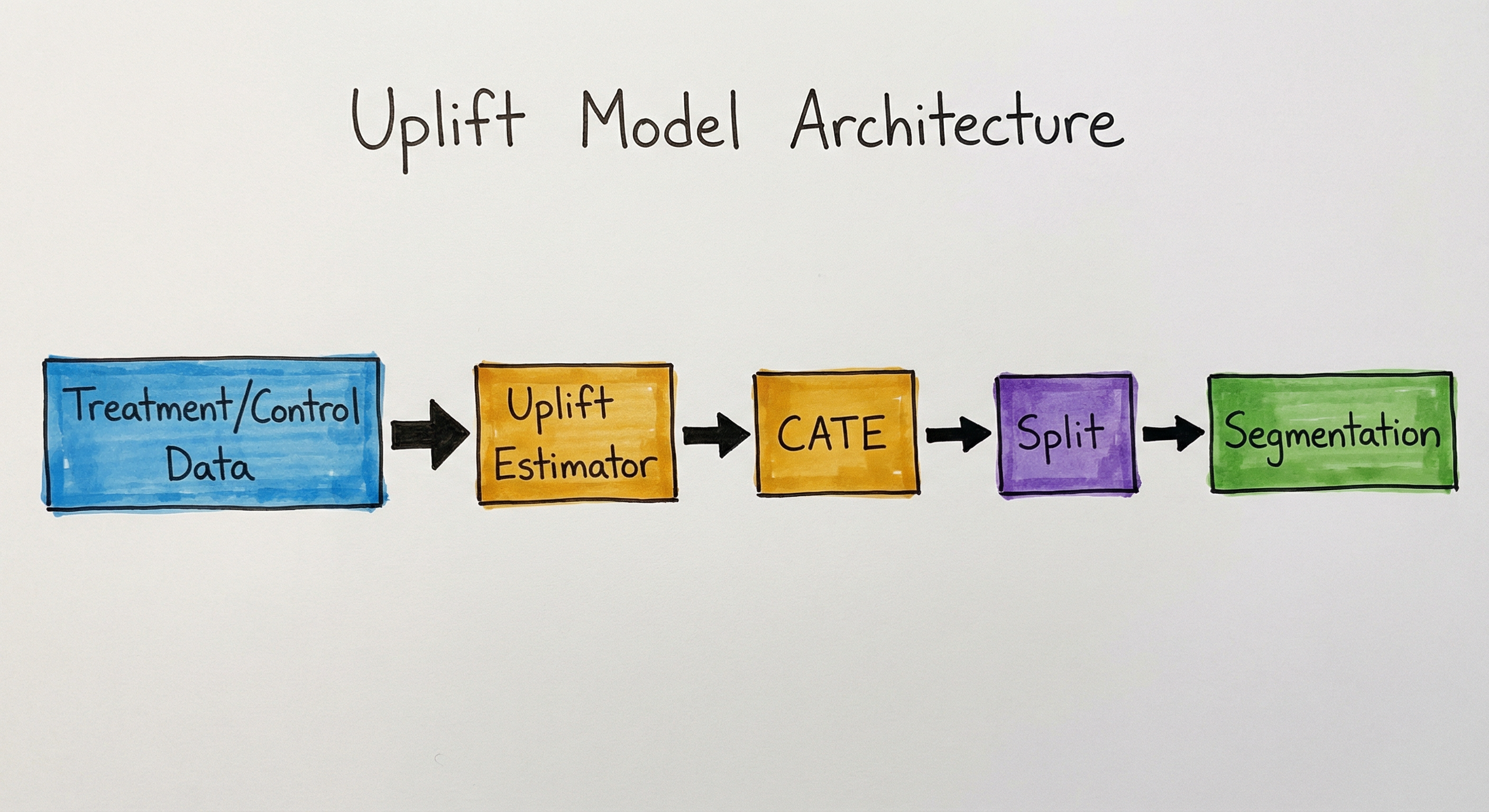
Internal Architecture
An uplift modeling system consists of four major stages: (1) experimental data collection via randomized trials, (2) CATE estimation using meta-learner or direct estimation methods, (3) model evaluation using uplift-specific metrics, and (4) targeting policy deployment that allocates treatments based on predicted uplift scores.
The architecture forms a closed loop: A/B test data feeds CATE estimation, which produces uplift scores for evaluation, which informs the targeting policy, which determines treatment allocation in the next campaign, and outcomes are monitored to feed back into the next iteration. This loop is critical because uplift models degrade if the targeting population shifts or if treatment effects change over time (concept drift in the causal sense).
Key Components
Experiment Data Collector
Ingests data from randomized A/B tests or quasi-experiments. Ensures proper randomization was maintained (balance checks), records treatment assignment , outcome , and covariates for each individual. In observational settings, also computes propensity scores for inverse probability weighting.
Feature Engineering Pipeline
Constructs features relevant to treatment effect heterogeneity, not just outcome prediction. This is a subtle but critical distinction: features that predict the outcome (e.g., past purchase count) may not predict the treatment effect (e.g., sensitivity to discounts). Interaction features between user attributes and treatment-related variables are often informative.
CATE Estimator (Meta-Learner)
The core model component. Implements one or more meta-learner strategies (S-learner, T-learner, X-learner, R-learner) or direct methods (causal forests, uplift trees). Takes triples and outputs a function mapping features to predicted uplift. Can wrap any base learner (XGBoost, random forest, neural network).
Propensity Score Estimator
Estimates , the probability of treatment given features. In randomized experiments with 50/50 split, this is trivially 0.5. In observational data or experiments with non-uniform assignment, accurate propensity estimation is critical for the X-learner's weighting and the R-learner's orthogonalization. Usually implemented as a logistic regression or gradient-boosted classifier.
Uplift Evaluation Module
Computes uplift-specific metrics: Qini curve, uplift curve, AUUC, Qini coefficient, and calibration plots. Unlike standard ML metrics, these must account for the fact that individual-level ground truth (the ITE) is never observed. Evaluation relies on comparing group-level outcomes sorted by predicted uplift -- if the model is good, targeting the top-K by predicted uplift should yield higher incremental conversions than random targeting.
Targeting Policy Engine
Converts uplift scores into actionable targeting decisions. In the simplest case, treat everyone with . With budget constraints, treat the top-K by uplift score. With multiple treatments and costs, solve an optimization problem: maximize total uplift subject to budget constraints (). This is where Uber's Net Value CATE formulation becomes relevant.
Outcome Monitor
Tracks post-deployment outcomes to validate that realized uplift matches predicted uplift. Implements holdout-based validation: a random subset continues to receive random treatment/control assignment even after the targeting policy is deployed, providing an ongoing ground truth for model calibration. Detects model drift when predicted vs. realized uplift diverges.
Data Flow
Step 1 -- Experiment Execution: Run a randomized A/B test where individuals are randomly assigned to treatment () or control (). Record features , assignment , and outcome for all individuals.
Step 2 -- Data Preparation: Join experiment data with feature tables. Compute derived features (recency, frequency, monetary for e-commerce; clinical history for healthcare). Split into train/validation/test sets, preserving the treatment/control ratio in each split.
Step 3 -- CATE Estimation: Apply one or more meta-learner algorithms. For T-learner: train separate outcome models on treatment and control subsets, predict on validation set, compute difference. For X-learner: additionally compute imputed treatment effects and train second-stage models.
Step 4 -- Evaluation: Sort validation set by predicted uplift (highest to lowest). Compute Qini curve by plotting cumulative incremental conversions vs. fraction targeted. Calculate AUUC and Qini coefficient. Compare against random targeting baseline and (if available) other models.
Step 5 -- Policy Construction: Given budget constraints and uplift scores, determine the targeting threshold. For example: "Treat the top 20% by uplift score" or "Treat everyone with predicted uplift > 0.03."
Step 6 -- Deployment: Score incoming individuals in real time (or batch), apply the targeting policy, and execute the treatment. Maintain a random holdout (5-10%) receiving random assignment for ongoing evaluation.
Step 7 -- Monitoring: Periodically compare predicted uplift to realized uplift in the holdout group. Trigger retraining if calibration degrades or if the targeting population shifts significantly.
A closed-loop flow: A/B test data feeds feature engineering, which feeds CATE estimation via meta-learners (S/T/X/R-learner). Uplift scores are evaluated using Qini/AUUC metrics, then consumed by a targeting policy engine that allocates treatments. Outcome monitoring feeds back to the experiment data stage for continuous improvement.
How to Implement
Implementing Uplift Models in Practice
Uplift modeling implementation breaks into three phases: (1) data preparation from A/B tests, (2) CATE estimation using meta-learner frameworks, and (3) evaluation with uplift-specific metrics.
The most common mistake practitioners make is jumping straight to complex methods (causal forests, deep learning) without first establishing baselines with simple meta-learners. Start with a T-learner using XGBoost as base learner -- it is simple, interpretable, and often surprisingly competitive. Then try the X-learner which typically improves on T-learner when treatment and control groups are imbalanced or when treatment effects are small. Only move to R-learner or doubly robust methods when you need robustness to model misspecification.
For evaluation, never use standard classification metrics (AUC-ROC, precision, recall) on uplift problems. These metrics evaluate outcome prediction, not treatment effect estimation. Instead, use the Qini curve and AUUC -- the uplift equivalents of ROC and AUC.
Infrastructure Considerations
For a system handling 10M users at a company like Swiggy or PhonePe, batch scoring is typical: run the uplift model nightly, generate uplift scores for all eligible users, and feed into the campaign management system. Real-time scoring is needed for dynamic treatments (e.g., showing/hiding a discount at checkout), requiring the model to be served via a low-latency endpoint.
Cost Note: Training an uplift model on 5M user-experiment records with XGBoost base learners takes approximately 10-15 minutes on a 16-core machine. Cloud compute cost: roughly ₹500-1000 ($6-12) on AWS/GCP per training run. Evaluation (Qini curve computation) adds negligible overhead. The real cost is in the A/B test itself -- running a proper experiment with sufficient sample size for a week on a platform with 10M DAU costs opportunity cost of suboptimal targeting during the test period.
import numpy as np
import pandas as pd
from sklearn.model_selection import train_test_split
from xgboost import XGBClassifier

# Simulate A/B test data
np.random.seed(42)
n = 10000
X = np.random.randn(n, 5)  # 5 features
T = np.random.binomial(1, 0.5, n)  # 50/50 randomization
# True CATE depends on X[:,0]: persuadables have high X[:,0]
true_cate = 0.1 * X[:, 0] + 0.05 * X[:, 1]
baseline = 1 / (1 + np.exp(-(-1 + 0.5 * X[:, 2])))
prob_y = baseline + T * true_cate
Y = np.random.binomial(1, np.clip(prob_y, 0, 1))

df = pd.DataFrame(X, columns=[f'x{i}' for i in range(5)])
df['treatment'] = T
df['outcome'] = Y

# Split data
train, test = train_test_split(df, test_size=0.3, random_state=42)

# T-Learner: separate models for treatment and control
feature_cols = [f'x{i}' for i in range(5)]

# Model for treatment group
treated = train[train['treatment'] == 1]
model_t = XGBClassifier(n_estimators=100, max_depth=4, random_state=42)
model_t.fit(treated[feature_cols], treated['outcome'])

# Model for control group
control = train[train['treatment'] == 0]
model_c = XGBClassifier(n_estimators=100, max_depth=4, random_state=42)
model_c.fit(control[feature_cols], control['outcome'])

# Predict uplift = P(Y=1|T=1,X) - P(Y=1|T=0,X)
uplift_scores = (
    model_t.predict_proba(test[feature_cols])[:, 1]
    - model_c.predict_proba(test[feature_cols])[:, 1]
)

test = test.copy()
test['uplift_score'] = uplift_scores
print(f"Mean predicted uplift: {uplift_scores.mean():.4f}")
print(f"Uplift score range: [{uplift_scores.min():.4f}, {uplift_scores.max():.4f}]")
This is the simplest uplift approach: train two separate outcome models (one on treated, one on control), predict with both, and subtract. The T-learner is easy to implement and understand, but it optimizes each model for outcome prediction rather than treatment effect estimation. Small errors in each model can compound when subtracted. Use this as your baseline before trying more advanced methods.
from causalml.inference.meta import BaseXClassifier
from xgboost import XGBClassifier
from sklearn.linear_model import LogisticRegression
import numpy as np

# Using the same simulated data from above
# X: features, T: treatment, Y: outcome

# X-Learner with XGBoost base learner
learner_x = BaseXClassifier(
    learner=XGBClassifier(n_estimators=100, max_depth=4, random_state=42),
    control_name='control'
)

# Format treatment column: 'treatment' or 'control'
treatment_labels = np.where(T == 1, 'treatment', 'control')

# Fit and predict CATE
cate_x = learner_x.estimate_ate(
    X=X, treatment=treatment_labels, y=Y
)
print(f"Estimated ATE: {cate_x[0][0]:.4f}")

# Get individual-level predictions
cate_individual = learner_x.fit_predict(
    X=X, treatment=treatment_labels, y=Y
)
print(f"Individual CATE range: [{cate_individual.min():.4f}, {cate_individual.max():.4f}]")
print(f"Fraction with positive uplift: {(cate_individual > 0).mean():.2%}")
The X-learner from CausalML uses a three-stage process: (1) fit outcome models on each group, (2) compute imputed treatment effects using cross-group predictions, (3) fit second-stage models on these imputed effects, and combine using propensity score weighting. It excels when treatment and control groups are imbalanced or when the true CATE is simpler than the outcome function -- both common in practice.
from sklift.metrics import (
    qini_auc_score,
    uplift_auc_score,
    qini_curve,
    uplift_curve
)
from sklift.viz import plot_qini_curve, plot_uplift_curve
import matplotlib.pyplot as plt
import numpy as np

# Assume we have:
# y_true: actual outcomes (0/1)
# uplift_scores: predicted uplift from our model
# treatment: treatment assignment (0/1)

# Example data
np.random.seed(42)
n = 5000
treatment = np.random.binomial(1, 0.5, n)
y_true = np.random.binomial(1, 0.3 + 0.1 * treatment, n)
uplift_scores = np.random.randn(n) * 0.2 + 0.1 * treatment

# Compute Qini coefficient (area between model curve and random)
qini_coeff = qini_auc_score(y_true, uplift_scores, treatment)
print(f"Qini coefficient: {qini_coeff:.4f}")

# Compute AUUC
auuc = uplift_auc_score(y_true, uplift_scores, treatment)
print(f"AUUC: {auuc:.4f}")

# Plot Qini curve
fig, axes = plt.subplots(1, 2, figsize=(14, 5))

# Qini curve
plot_qini_curve(y_true, uplift_scores, treatment, ax=axes[0])
axes[0].set_title('Qini Curve')

# Uplift curve
plot_uplift_curve(y_true, uplift_scores, treatment, ax=axes[1])
axes[1].set_title('Uplift Curve')

plt.tight_layout()
plt.savefig('uplift_evaluation.png', dpi=150)
plt.show()
The Qini curve plots cumulative incremental conversions (treatment minus scaled control) as you target more of the population, sorted by predicted uplift from highest to lowest. A good model produces a curve that rises steeply (high-uplift individuals targeted first) and then flattens (low-uplift or negative-uplift individuals targeted last). The Qini coefficient is the area between this curve and the random targeting diagonal. The uplift curve similarly shows the difference in conversion rates between treatment and control groups within each decile.
from econml.dr import ForestDRLearner
from sklearn.ensemble import GradientBoostingClassifier, GradientBoostingRegressor
import numpy as np

# Simulated data
np.random.seed(42)
n = 10000
X = np.random.randn(n, 5)
T = np.random.binomial(1, 0.5, n)
true_cate = 0.1 * X[:, 0] + 0.05 * X[:, 1]
baseline = 1 / (1 + np.exp(-(-1 + 0.5 * X[:, 2])))
Y = baseline + T * true_cate + np.random.randn(n) * 0.1

# Doubly Robust Forest Learner
# Robust to misspecification of either outcome or propensity model
dr_learner = ForestDRLearner(
    model_regression=GradientBoostingRegressor(n_estimators=100, max_depth=4),
    model_propensity=GradientBoostingClassifier(n_estimators=100, max_depth=3),
    n_estimators=200,
    min_samples_leaf=10,
    random_state=42
)

# Fit
dr_learner.fit(Y, T, X=X)

# Predict CATE with confidence intervals
cate_pred = dr_learner.effect(X)
cate_lower, cate_upper = dr_learner.effect_interval(X, alpha=0.05)

print(f"Mean predicted CATE: {cate_pred.mean():.4f}")
print(f"True ATE: {true_cate.mean():.4f}")
print(f"95% CI width (avg): {(cate_upper - cate_lower).mean():.4f}")

# Feature importance for treatment effect heterogeneity
importances = dr_learner.feature_importances_
for i, imp in enumerate(importances):
    print(f"Feature x{i}: importance = {imp:.4f}")
The ForestDRLearner from EconML combines doubly robust estimation with generalized random forests. It is robust to misspecification of either the outcome model or the propensity model (as long as at least one is correct). This is a significant advantage over T-learner and X-learner, which rely on accurate outcome models. The method also provides confidence intervals for individual CATE estimates, which is valuable for decision-making under uncertainty. Feature importances indicate which variables drive treatment effect heterogeneity -- these are often different from the features that drive outcomes.
from causalml.inference.meta import BaseTClassifier
from xgboost import XGBClassifier
import numpy as np
import pandas as pd

# Simulate multi-treatment scenario:
# Treatment 0: Control (no action)
# Treatment 1: Push notification (cost = INR 0.5)
# Treatment 2: Email campaign (cost = INR 2)
# Treatment 3: Discount coupon (cost = INR 50)

np.random.seed(42)
n = 20000
X = np.random.randn(n, 5)
treatments = np.random.choice(['control', 'push', 'email', 'coupon'], n)

# Simulate outcomes with different treatment effects
baseline = 0.1
effects = {
    'control': 0,
    'push': 0.02 + 0.01 * X[:, 0],
    'email': 0.05 + 0.02 * X[:, 1],
    'coupon': 0.15 + 0.03 * X[:, 0] + 0.02 * X[:, 2]
}
probs = baseline + np.array([effects[t][i] for i, t in enumerate(treatments)])
Y = np.random.binomial(1, np.clip(probs, 0, 1))

# Cost per treatment
costs = {'push': 0.5, 'email': 2.0, 'coupon': 50.0}  # INR
revenue_per_conversion = 500  # INR

# Fit multi-treatment T-learner
learner = BaseTClassifier(
    learner=XGBClassifier(n_estimators=100, max_depth=4, random_state=42),
    control_name='control'
)
cate_multi = learner.fit_predict(X=X, treatment=treatments, y=Y)

# cate_multi has columns for each treatment vs control
# Compute Net Value CATE = (CATE * revenue) - cost
for i, trt in enumerate(['coupon', 'email', 'push']):
    net_value = cate_multi[:, i] * revenue_per_conversion - costs[trt]
    print(f"{trt}: mean CATE={cate_multi[:, i].mean():.4f}, "
          f"mean Net Value=INR {net_value.mean():.2f}")

# Optimal treatment assignment: pick treatment with highest net value
# (or control if all net values are negative)
net_values = np.column_stack([
    cate_multi[:, i] * revenue_per_conversion - costs[trt]
    for i, trt in enumerate(['coupon', 'email', 'push'])
])
net_values = np.column_stack([np.zeros(n), net_values])  # add control (0)
treatment_names = ['control', 'coupon', 'email', 'push']
optimal = np.argmax(net_values, axis=1)
for i, name in enumerate(treatment_names):
    print(f"Assigned to {name}: {(optimal == i).sum()} users ({(optimal == i).mean():.1%})")
This implements Uber's Net Value CATE framework for multi-treatment optimization. Instead of just maximizing uplift, we maximize net value: the expected incremental revenue from a conversion minus the cost of the treatment. A coupon might have a high CATE but also a high cost (INR 50), while a push notification has a low CATE but near-zero cost. The optimal policy assigns each user to the treatment that maximizes their net value -- which might be no treatment at all if all options have negative expected net value.
# CausalML X-Learner configuration
from causalml.inference.meta import BaseXClassifier
from xgboost import XGBClassifier

learner = BaseXClassifier(
    learner=XGBClassifier(
        n_estimators=200,
        max_depth=5,
        learning_rate=0.1,
        subsample=0.8,
        colsample_bytree=0.8,
        random_state=42
    ),
    control_name='control'  # Name of the control group in treatment column
)

# EconML ForestDRLearner configuration
from econml.dr import ForestDRLearner

dr_learner = ForestDRLearner(
    model_regression=GradientBoostingRegressor(n_estimators=200),
    model_propensity=GradientBoostingClassifier(n_estimators=100),
    n_estimators=500,          # Number of trees in the causal forest
    min_samples_leaf=20,       # Minimum samples per leaf (controls smoothness)
    max_depth=None,            # Let trees grow fully
    subsample_fr=0.7,          # Subsample fraction for honest splitting
    random_state=42
)
Common Implementation Mistakes
- ●
Using standard classification metrics (AUC-ROC, F1) for evaluation: Uplift models predict causal effects, not outcomes. A model with high outcome-prediction AUC can have terrible uplift discrimination. Always use Qini curves, AUUC, or uplift-specific calibration plots.
- ●
Training on biased (non-randomized) data without adjusting for confounding: If treatment assignment was not random (e.g., high-value customers got the coupon preferentially), your CATE estimates will be biased. Either use randomized experiment data or apply propensity score weighting / doubly robust methods.
- ●
Insufficient sample size for detecting small treatment effects: Uplift effects are typically much smaller than outcome effects (e.g., CATE = 0.02 vs. baseline conversion = 0.10). You need 5-10x more data than for a standard classification task to achieve the same statistical power for uplift estimation.
- ●
Ignoring the Do Not Disturb segment: Some individuals have negative treatment effects -- targeting them actively destroys value. If your model only predicts positive uplift (e.g., by clipping at 0), you miss the opportunity to protect these users from harmful interventions. Always check for and respect negative uplift predictions.
- ●
Overfitting to treatment-outcome correlations in observational data: Without proper causal identification (randomization or strong instrumental variables), your uplift model may learn spurious treatment-outcome associations. The gold standard is always randomized experimental data.
- ●
Neglecting treatment-control ratio balance in splits: When splitting data for train/test, ensure each split maintains the original treatment/control ratio. Stratified splitting on the treatment variable is essential -- otherwise your CATE estimates will be biased in some splits.
When Should You Use This?
Use When
You have randomized A/B test data with treatment and control groups and want to optimize whom to target in future campaigns, not just measure the average treatment effect
Marketing or product budgets are limited and you need to allocate interventions (coupons, notifications, discounts) to the subset of users who will benefit most
You suspect significant treatment effect heterogeneity -- the treatment works well for some users but not others, and you want to identify and exploit these subgroups
The cost of treatment is non-trivial (e.g., ₹50 discount coupons, ₹500 referral bonuses, expensive medical therapies) and you want to maximize return on investment by targeting persuadables
You want to avoid the Do Not Disturb segment -- users who will be negatively affected by the treatment (e.g., over-notified users who churn, patients with adverse drug reactions)
Your organization is mature enough to run proper randomized experiments and has sufficient data volume (typically 50K+ observations per treatment arm for reliable CATE estimation)
Avoid When
You do not have randomized experimental data and cannot credibly estimate propensity scores -- uplift models on confounded observational data produce misleading results
Treatment is free, universal, and has no negative effects -- if you can treat everyone at zero cost with no downside, just treat everyone; no need for uplift modeling
Sample size is too small to detect heterogeneous treatment effects -- with fewer than 10K observations per arm, meta-learners often produce noisy, unreliable CATE estimates
The treatment effect is known to be homogeneous (affects everyone equally) -- if CATE is constant across the population, a simple ATE estimate from a t-test is sufficient
You need real-time, per-request decisions and lack the infrastructure for model serving -- uplift models add complexity over simple response models, requiring careful deployment
Your A/B test has severe compliance issues (high non-compliance, crossover between treatment and control) that violate SUTVA and invalidate causal effect estimates
Key Tradeoffs
Complexity vs. Targeting Precision
The simplest targeting approach is a response model: rank users by P(conversion) and target the top-K. This is wrong (targets Sure Things, not Persuadables) but easy. The next step is a T-learner: two models, subtract predictions. This is better but noisy. X-learner and R-learner improve precision but add complexity. Doubly robust methods (EconML's ForestDRLearner) offer robustness guarantees but require more engineering and computational resources.
| Method | Complexity | When It Excels |
|---|---|---|
| Response model (no uplift) | Low | Never for targeting -- serves as negative baseline |
| S-learner | Low | Simple treatment effects, regularized base learners |
| T-learner | Medium | Balanced groups, large treatment effects |
| X-learner | Medium-High | Imbalanced groups, small effects, simple CATE |
| R-learner | High | Observational data, robustness needed |
| Doubly Robust (DR) | High | Misspecification concerns, confidence intervals needed |
| Causal Forest | High | Non-parametric CATE, interpretable heterogeneity |
Statistical Power vs. Granularity
Uplift effects are inherently noisier than outcome predictions because you are estimating a difference between two noisy quantities. This means you need significantly more data for uplift modeling than for standard classification. A rule of thumb: if you need 10K samples for a good binary classifier, expect to need 50K-100K for reliable individual-level uplift estimation.
You can trade granularity for power: instead of estimating individual-level CATE, estimate CATE for segments (e.g., high-value vs. low-value users). Segment-level uplift is more robust but less precise. Start with 5-10 segments, validate that uplift ordering is consistent across holdout sets, and only move to individual-level if your data supports it.
Model Interpretability vs. Performance
Uplift trees and causal forests offer direct interpretability: "Users with X > 0.5 and Y < 3 have the highest treatment effect." Neural-network-based uplift models (DragonNet, CEVAE) may achieve better CATE estimation on complex data but are harder to explain to stakeholders. In regulated industries (banking, healthcare), interpretability often trumps marginal performance gains.
Practical Advice: Start with T-learner + XGBoost as your baseline. If it shows meaningful uplift discrimination (Qini coefficient significantly above zero), you have signal. Then try X-learner or DR-learner for improvement. If the baseline Qini is near zero, investigate whether your features contain treatment effect heterogeneity at all before investing in more complex methods.
Alternatives & Comparisons
A/B testing estimates the Average Treatment Effect (ATE) -- the mean impact across the entire population -- while uplift modeling estimates the Conditional Average Treatment Effect (CATE) -- the impact for each individual or subgroup. A/B testing answers 'does the treatment work on average?' whereas uplift modeling answers 'for whom does the treatment work best?' Use A/B testing when you only need a go/no-go decision on a treatment. Use uplift modeling when you need to optimize whom to target with a treatment that has heterogeneous effects.
Statistical significance testing (t-tests, chi-squared tests, bootstrap tests) determines whether an observed treatment effect is likely due to chance. It complements uplift modeling by providing confidence in the ATE estimate and in subgroup-level CATE estimates. Significance testing alone tells you 'the effect is real' but not 'who benefits most.' Uplift modeling tells you 'who benefits most' but you still need significance testing to confirm the heterogeneity is not noise. Use both together: significance testing for validation, uplift modeling for targeting.
ROC-AUC evaluates a model's ability to rank individuals by outcome probability, while Qini/AUUC evaluates a model's ability to rank individuals by treatment effect. A high-AUC response model identifies who will convert, but this is the wrong optimization target for targeting decisions because it conflates Sure Things with Persuadables. Use ROC-AUC for outcome prediction; use Qini/AUUC for treatment allocation. They measure fundamentally different things -- optimizing one does not optimize the other.
Like ROC-AUC, precision-recall-F1 evaluates outcome prediction quality, not treatment effect estimation. A model with perfect precision and recall for identifying converters would still be a poor uplift model if it cannot distinguish Persuadables from Sure Things. Precision-recall-F1 and uplift metrics live in different evaluation universes. Use precision-recall when predicting who will convert; use Qini/AUUC when deciding who to treat.
Pros, Cons & Tradeoffs
Advantages
Directly optimizes the business objective of targeting persuadables rather than predicting outcomes, which can dramatically improve campaign ROI -- published case studies show 20-50% improvement in incremental conversions compared to response-model-based targeting
Identifies the Do Not Disturb segment -- individuals who are harmed by treatment (negative CATE) -- protecting against value destruction from over-targeting, which response models completely miss
Flexible meta-learner framework allows wrapping any supervised learning algorithm (XGBoost, neural networks, random forests) as a base learner, meaning you can leverage your existing ML infrastructure and expertise
Well-supported open-source ecosystem with CausalML (Uber), EconML (Microsoft), scikit-uplift, and DoWhy providing production-grade implementations with active maintenance and community support
Natural extension of A/B testing -- if your organization already runs experiments, uplift modeling extracts strictly more value from the same data by decomposing the ATE into individual-level effects
Enables budget-constrained optimization through Net Value CATE formulations that account for treatment costs, allowing optimal allocation of limited marketing or intervention budgets across heterogeneous populations
Provides causal (not correlational) targeting -- under proper experimental design, uplift estimates reflect genuine causal effects, making targeting decisions defensible and interpretable to stakeholders
Disadvantages
Requires randomized experimental data (or strong quasi-experimental designs) for valid causal identification -- organizations that cannot run A/B tests or lack historical experiment data cannot reliably use uplift modeling
Fundamentally noisier than outcome prediction because CATE is a difference of two noisy estimates, demanding 5-10x more data than standard classification to achieve comparable precision in estimates
No individual-level ground truth exists -- you can never observe the ITE for a single individual (fundamental problem of causal inference), making model debugging and error analysis significantly harder than for standard ML
Evaluation metrics (Qini, AUUC) are non-normalized -- unlike AUC-ROC which ranges from 0.5 to 1.0, Qini coefficient values depend on the dataset, making cross-dataset comparisons and absolute thresholds difficult to establish
Complex model selection and hyperparameter tuning -- you cannot simply use cross-validated RMSE or AUC; you need uplift-specific validation strategies, and the optimal meta-learner choice depends on unknown properties of the true CATE function
Risk of overfitting to heterogeneity noise -- with small treatment effects and limited data, uplift models can learn spurious treatment-feature interactions that do not generalize, leading to targeting policies that underperform random assignment
Failure Modes & Debugging
CATE Overfitting on Small Treatment Effects
Cause
When the true treatment effect is small relative to outcome variance (common in marketing: CATE = 0.01-0.03 on baseline conversion of 0.10-0.30), meta-learners pick up noise in the treatment-feature interactions rather than true heterogeneity. This is exacerbated by high-dimensional feature spaces and insufficient sample size per treatment arm.
Symptoms
High Qini coefficient on training data but near-zero or negative Qini on holdout data. Predicted uplift scores show extreme variance (some predictions at +0.30, others at -0.20) despite true CATE having a much narrower range. Targeting the top decile by predicted uplift yields no better incremental conversions than random targeting in production.
Mitigation
Use regularization in base learners (lower max_depth, higher min_samples_leaf for tree-based models). Perform honest splitting (separate data for splitting and estimation, as in causal forests). Validate on multiple holdout sets and check if the uplift ordering is consistent. Consider segment-level CATE (5-10 segments) instead of individual-level if data is limited. Use cross-validated Qini for model selection.
Confounding Bias in Observational Data
Cause
When treatment assignment is not randomized, observed differences between treated and control groups may reflect selection bias rather than causal effects. For example, if high-value customers are more likely to receive a promotional coupon (because the business already targets them), the model will overestimate CATE for high-value segments.
Symptoms
Predicted CATE is suspiciously large (e.g., 0.15 when prior experiments suggest ATE = 0.03). CATE correlates strongly with features known to influence treatment assignment (e.g., customer lifetime value, engagement score). Propensity model AUC is very high (>0.9), indicating treatment assignment is highly predictable from features -- a red flag for confounding.
Mitigation
Strongly prefer randomized experimental data. If observational data is unavoidable, use doubly robust methods (R-learner, ForestDRLearner) that are robust to misspecification of either the outcome or propensity model. Perform sensitivity analysis (e.g., Rosenbaum bounds) to assess how much hidden confounding would be needed to explain your results. Consider instrumental variable approaches if valid instruments are available.
Violations of SUTVA (Interference Between Units)
Cause
SUTVA assumes one individual's treatment does not affect another's outcome. This is violated in network settings (social media campaigns where treated users influence untreated friends), marketplace settings (treating one seller affects competing sellers), and limited-inventory settings (coupon redemptions deplete stock, affecting others). Ride-hailing platforms like Ola or Uber face this acutely: offering a discount to one rider affects driver availability for others.
Symptoms
Estimated ATE from uplift model differs significantly from the ATE measured in a properly designed cluster-randomized experiment. Uplift estimates for individuals in dense social networks are systematically higher than for isolated individuals. Treatment effects diminish when the targeting fraction increases (interference dilutes per-person impact).
Mitigation
Use cluster-randomized experiments (randomize at the city, market, or network-cluster level) instead of individual randomization. Apply interference-aware estimators that model spillover effects. Run holdout validation comparing predicted uplift at different targeting fractions -- if the Qini curve shape changes dramatically with targeting percentage, interference is likely present.
Temporal Drift in Treatment Effects
Cause
Treatment effects change over time due to market dynamics, user behavior shifts, competitive actions, or saturation. A coupon campaign that had strong uplift in Q1 may have diminished effect in Q3 because competitors matched the offer, or because the persuadable segment has already been converted. Seasonal effects (Diwali sales in India, holiday season globally) further complicate temporal stability.
Symptoms
Qini coefficient on recent data is significantly lower than on training data from 3-6 months ago. Targeting policy based on old uplift scores underperforms random assignment in production A/B tests. The proportion of users with positive predicted uplift changes substantially across time periods despite similar populations.
Mitigation
Retrain uplift models regularly (monthly or per-campaign for fast-moving domains like e-commerce). Maintain an always-on randomized holdout (5-10% of traffic) to continuously estimate realized uplift and detect drift. Use time-weighted training where recent experiments receive higher weight. Consider online/adaptive uplift models that update incrementally.
Evaluation Metric Gaming via Outcome Prediction
Cause
Practitioners evaluate their uplift model using Qini/AUUC but then realize that a strong outcome prediction model (which is not an uplift model) can sometimes achieve reasonable Qini scores by coincidence -- if outcome-predictive features happen to correlate with treatment heterogeneity. This leads to false confidence that the model is doing genuine uplift estimation.
Symptoms
Qini coefficient is positive but comparable to what a simple response model achieves. Uplift scores are highly correlated (Pearson > 0.8) with outcome predictions P(Y=1|X). The model assigns high uplift to high-baseline-probability individuals rather than to those with genuine treatment effect heterogeneity. Removing the treatment variable from the model does not significantly change Qini.
Mitigation
Always compare your uplift model's Qini against a response-model baseline (train a standard classifier, use its predictions as 'uplift scores'). If your uplift model does not substantially outperform this baseline, it is not capturing genuine treatment heterogeneity. Perform a synthetic data validation: generate data with known CATE function, verify your model recovers it. Check that the top-uplift segment has a meaningfully higher treatment-control outcome gap than the bottom segment.
Placement in an ML System
Where Does Uplift Modeling Fit in the ML Pipeline?
Uplift modeling sits at the intersection of experimentation and targeting/personalization -- it consumes experimental data and produces targeting policies.
Upstream Dependencies: The primary input is data from an A/B test runner that has properly randomized individuals into treatment and control groups. Statistical significance testing validates that the overall ATE is meaningful before investing in heterogeneous effect estimation. A feature store provides user-level features (demographics, behavioral history, engagement metrics) that drive treatment effect heterogeneity.
The Uplift Modeling Stage: Given experiment data and features, the uplift model estimates individual-level CATE using meta-learner algorithms. This stage includes training, evaluation (Qini/AUUC), and model selection. The output is a trained model that can score any user with a predicted uplift value.
Downstream Consumption: Uplift scores feed into a targeting policy engine that determines which users receive treatment in the next campaign. This policy is deployed via the campaign management system (for batch campaigns like email/push) or via a model serving endpoint (for real-time decisions like showing/hiding a discount at checkout). A monitoring dashboard tracks predicted vs. realized uplift to detect model drift.
Feedback Loop: Critically, the targeting policy influences future experimental data. If you only treat high-uplift users, you lose information about low-uplift users (exploration-exploitation tradeoff). Maintaining a randomized holdout (5-10% receiving random assignment) ensures ongoing model evaluation and retraining data.
Production Pattern: At companies like Uber and Booking.com, uplift models run as nightly batch jobs that score the full user base. Scores are written to a feature store and consumed by the campaign system. A smaller real-time uplift model handles dynamic decisions (e.g., showing a surge pricing explanation to users predicted to churn vs. those who will accept).
Pipeline Stage
Evaluation / Experimentation / Targeting Optimization
Upstream
- ab-test-runner
- statistical-significance
- feature-store
Downstream
- notification-service
- campaign-management
- model-serving-endpoint
- monitoring-dashboard
Scaling Bottlenecks
Training: Meta-learners multiply the training cost by 2-3x compared to a single model. A T-learner trains two separate models; an X-learner trains four (two outcome models + two imputed-effect models). For XGBoost base learners on 10M rows with 50 features, expect 20-40 minutes on a 16-core instance (e.g., AWS m5.4xlarge at ~₹100/hour). With cross-validation for meta-learner selection across 4 methods x 5 folds, total training time approaches 2-4 hours.
Inference/Scoring: For T-learner, each prediction requires two model inferences (treatment and control predictions). At 50K predictions/second with XGBoost on CPU, this means 25K uplift scores/second. For batch scoring 10M users, budget 7-10 minutes. For real-time scoring at checkout (e.g., dynamic coupon decisioning at Flipkart), p99 latency must stay under 50ms -- deploy both models behind a single endpoint and parallelize the two inferences.
Evaluation: Qini curve computation requires sorting all predictions and sweeping through the sorted list -- . For M, this is ~5 seconds. Bootstrapped confidence intervals on Qini (2000 resamples) take 15-30 minutes. Use parallel bootstrap on multiple CPU cores.
Data Storage: Experiment data must be retained with full treatment assignment and outcome records. For a 10M-user experiment with 50 features, this is approximately 4-8 GB in Parquet format. Historical experiment archives (for retraining) can grow to 50-100 GB over a year.
Production Case Studies
Uber developed the CausalML open-source library and pioneered multi-treatment uplift modeling with cost optimization for rider and driver promotions. Their system estimates CATE across multiple treatment types (push notification, email, discount coupon, referral bonus) with different costs, then optimizes targeting by maximizing Net Value CATE = (CATE x revenue) - treatment cost. This allows Uber to decide not just whether to treat a user but which treatment to apply, accounting for ROI.
Uber reported that uplift-based targeting improved campaign ROI by 20-30% compared to response-model-based targeting across rider acquisition and driver retention campaigns. The CausalML library has been adopted by thousands of organizations globally and is one of the most-starred causal inference packages on GitHub (4,500+ stars).
Booking.com implemented retrospective uplift modeling for dynamic promotions recommendation within ROI constraints. Their approach uses a Knapsack Problem formulation to optimally allocate personalized discounts to hotel bookers, maximizing incremental bookings while staying within a fixed promotional budget. They introduced Retrospective Estimation, which relies solely on positive-outcome data, simplifying the modeling pipeline.
Online A/B tests at Booking.com showed the uplift-based personalized promotions group achieved a cumulative uplift of 66% of the fully-treated group at significantly lower cost. The personalized group maintained consistently high ROI (0.36 at the final measurement period), substantially outperforming blanket promotion strategies. The system was deployed to millions of customers globally.
Wayfair applied uplift modeling to display remarketing -- deciding which users should receive Wayfair ads across the internet. They designed randomized experiments where customers were assigned to either see Wayfair ads (treatment) or public service announcements (control). The uplift model, combined with a real-time bidding algorithm, determined individual-level bids based on predicted incremental purchase probability.
Wayfair's uplift-optimized bidding strategy allocated ad spend to users with the highest incremental purchase lift, resulting in measurable improvements in marketing efficiency. The system combined user-level uplift predictions with inventory-level click-through rate models, forming a full real-time bidding pipeline that continuously optimized return on ad spend (ROAS) across the display advertising ecosystem.
Swiggy implemented heterogeneous treatment effect evaluation for coupon targeting and customer retention campaigns. In India's hypercompetitive food delivery market (Swiggy vs. Zomato), efficiently allocating promotional budgets is critical: a ₹100 coupon that attracts a ₹200 order from a customer who would have ordered anyway is a net loss. Swiggy's uplift approach identifies users whose ordering frequency genuinely increases due to the coupon, rather than users who simply have high baseline order frequency.
By moving from response-model targeting to uplift-based targeting, Indian food delivery platforms have reported 15-25% improvements in incremental order volume per rupee spent on promotions. For a platform like Swiggy spending ₹500-1000 crore annually on promotions, even a 10% efficiency gain translates to ₹50-100 crore ($6-12M) in recovered marketing budget or additional incremental orders.
Nubank, Latin America's largest digital bank (70M+ customers), moved beyond simple prediction machines to causal inference for customer acquisition. Instead of just predicting who will convert, they built uplift models to identify customers whose behavior would actually change due to a marketing intervention, distinguishing between sure things (would convert anyway) and persuadables (need the nudge) (2021).
By shifting from predictive to causal models, Nubank achieved 30-40% improvement in marketing ROI by targeting only truly persuadable customers. The approach also reduced customer annoyance from irrelevant campaigns and became a core framework across their growth team.
Tooling & Ecosystem
The most comprehensive uplift modeling library. Implements S-learner, T-learner, X-learner, R-learner, doubly robust learner, uplift trees, and causal forests. Supports binary and multiple treatments, continuous and binary outcomes. Includes evaluation metrics (Qini, AUUC, cumulative gain), visualization tools, and sensitivity analysis. 4,500+ GitHub stars.
Microsoft's ALICE project library for heterogeneous treatment effect estimation. Implements Double Machine Learning, Forest Doubly Robust Learner, Orthogonal Random Forests, and meta-learners. Strong emphasis on confidence intervals and statistical inference for CATE. Integrates with Azure ML. Best choice when you need rigorous uncertainty quantification for individual treatment effects.
Lightweight, scikit-learn-compatible uplift modeling library. Implements Solo Model (S-learner), Two Models (T-learner), and Class Transformation approaches. Excellent evaluation module with qini_auc_score, uplift_auc_score, and publication-quality visualization functions (plot_qini_curve, plot_uplift_curve). Best for quick experimentation and evaluation.
Causal inference library focused on causal graph specification, identification, estimation, and refutation. While not uplift-specific, DoWhy provides the causal reasoning framework (identify valid adjustment sets, test causal assumptions) that should precede uplift modeling. Use DoWhy to validate your causal model before deploying CausalML/EconML estimators.
Google's TF-DF includes built-in uplift modeling support via honest causal forests and uplift-specific splitting criteria. Integrates natively with TensorFlow ecosystem. Suitable for teams already using TensorFlow who want uplift capabilities without adding another dependency.
Python package specifically designed for uplift modeling in real-world business settings. Supports both A/B testing data and observational data via propensity score adjustment. Provides a simple high-level API that automates the meta-learner training pipeline. Less feature-rich than CausalML but easier to get started with.
Research & References
Kunzel, Sekhon, Bickel & Yu (2019)Proceedings of the National Academy of Sciences (PNAS)
Seminal paper introducing the X-learner and formalizing the S-learner, T-learner, and R-learner meta-algorithms for CATE estimation. Shows that X-learner outperforms other meta-learners when treatment and control groups are imbalanced or when CATE is simpler than the outcome function. Provides theoretical convergence rates and extensive empirical evaluation.
Gutierrez & Gerardy (2017)Proceedings of Machine Learning Research (PMLR), Vol. 67
The first comprehensive review unifying the uplift modeling literature through the lens of the Rubin causal model. Covers the two-model approach, class transformation approach, and direct uplift modeling. Provides a clear taxonomy and comparison of methods with practical guidance on when to use each approach.
Zhao & Harinen (2019)IEEE International Conference on Data Science and Advanced Analytics (DSAA)
Introduces Net Value CATE for multi-treatment uplift optimization with treatment costs. Extends standard meta-learners to handle multiple treatment arms simultaneously and formulates the targeting decision as a constrained optimization problem. Describes Uber's production system architecture for causal uplift at scale.
Wager & Athey (2018)Journal of the American Statistical Association
Introduces causal forests -- an adaptation of random forests for CATE estimation with pointwise confidence intervals. Proves asymptotic normality of causal forest estimates under regularity conditions. The theoretical foundation for EconML's forest-based estimators and a major bridge between the causal inference and ML communities.
Radcliffe & Surry (2011)White Paper, Stochastic Solutions
Practical guide to uplift modeling from the pioneers of the field. Covers variable selection, model construction, quality measures, and post-campaign evaluation -- all requiring different approaches from traditional response modeling. Introduces significance-based uplift trees that directly optimize treatment effect heterogeneity at each split.
Goldenberg, Albert, Bernardi & Estevez (2020)ACM Conference on Recommender Systems (RecSys)
Booking.com's production uplift system for personalized promotions. Introduces Retrospective Estimation (modeling only on positive outcomes) and a Knapsack-based optimization for budget-constrained treatment allocation. Validated via online A/B tests showing significant revenue uplift at controlled cost.
Interview & Evaluation Perspective
Common Interview Questions
- ●
What is the difference between a response model and an uplift model? Why would you use one over the other for targeting?
- ●
Explain the four customer segments (Sure Things, Persuadables, Lost Causes, Do Not Disturb). How does uplift modeling help identify each?
- ●
Compare S-learner, T-learner, and X-learner. When would you choose each, and what are their relative strengths?
- ●
How do you evaluate an uplift model? Why can't you use standard metrics like AUC-ROC or F1?
- ●
What is the fundamental problem of causal inference, and how does uplift modeling work around it?
- ●
You have a ₹10 crore budget for promotional coupons. How would you design an uplift modeling system to maximize incremental revenue?
- ●
Your uplift model shows high Qini on training data but near-zero Qini on holdout. What went wrong and how do you fix it?
Key Points to Mention
- ●
Uplift modeling estimates CATE (the causal effect for each individual), not P(outcome). This requires experimental data and fundamentally different evaluation metrics (Qini, AUUC) rather than standard classification metrics.
- ●
The X-learner excels when treatment effects are small and groups are imbalanced because it uses cross-group imputation and propensity weighting. The R-learner directly targets CATE in its loss function, making it robust to outcome model misspecification.
- ●
The fundamental problem of causal inference means individual-level ground truth never exists -- you always evaluate at the group level by checking if high-predicted-uplift segments actually show larger treatment-control outcome gaps.
- ●
Always compare your uplift model against a response-model baseline on Qini/AUUC. If the uplift model does not substantially outperform, you may not have sufficient treatment effect heterogeneity in your features.
- ●
For multi-treatment settings with costs (realistic for most businesses), use Net Value CATE = (CATE x expected revenue) - treatment cost. The optimal policy assigns each user to the treatment that maximizes their net value.
- ●
Temporal drift in treatment effects is a major production challenge. Always maintain a randomized holdout (5-10%) for ongoing model evaluation and trigger retraining when predicted vs. realized uplift diverges.
Pitfalls to Avoid
- ●
Saying you would use AUC-ROC or F1 to evaluate an uplift model -- this is the most common red flag. Uplift requires Qini curves and AUUC, not standard classification metrics.
- ●
Claiming you can do uplift modeling on observational (non-randomized) data without discussing confounding, propensity adjustment, or sensitivity analysis -- shows lack of causal reasoning.
- ●
Ignoring the Do Not Disturb segment and only discussing positive uplift. Real uplift models produce negative predictions, and acknowledging this shows sophistication.
- ●
Conflating ATE (average treatment effect) with CATE (individual-level effect). ATE tells you the average impact; CATE tells you who benefits most. Uplift modeling is about CATE.
- ●
Not mentioning the data requirements -- uplift estimation needs significantly more data than outcome prediction because treatment effects are noisier. A 10K-sample A/B test may be sufficient for ATE but inadequate for individual-level CATE.
Senior-Level Expectation
A senior/staff-level candidate should demonstrate end-to-end system design for uplift-based targeting: from experiment design (sample size for heterogeneous effects, cluster randomization for interference-prone settings) through CATE estimation (meta-learner selection based on data properties) to policy deployment (budget-constrained optimization with Net Value CATE). They should articulate the exploration-exploitation tradeoff in targeting -- if you only treat high-uplift users, you lose ability to detect drift and retrain. They should discuss doubly robust methods and why they are preferable in observational settings. For India-specific context, they should quantify business impact: 'An uplift-optimized coupon campaign at Flipkart targeting 5 crore users with ₹100 coupons at 20% improved efficiency saves ₹100 crore annually.' They should also discuss practical failure modes like temporal drift, SUTVA violations in marketplace settings, and the challenge of evaluating models when ground truth is unobservable.
Summary
Uplift modeling solves the problem of deciding whom to treat rather than whether a treatment works. By estimating the Conditional Average Treatment Effect (CATE) for each individual, it identifies Persuadables -- those who convert only because of the intervention -- and separates them from Sure Things (would convert anyway), Lost Causes (will not convert regardless), and the Do Not Disturb segment (actively harmed by treatment). This is fundamentally different from response modeling, which conflates all four segments.
The technical approach centers on meta-learners: the S-learner (single model with treatment as feature), T-learner (separate models per group), X-learner (cross-group imputation with propensity weighting), and R-learner (direct CATE optimization via Robinson decomposition). More advanced methods like causal forests and doubly robust estimators provide additional robustness and confidence intervals. Evaluation uses Qini curves and AUUC -- the uplift analogues of ROC curves and AUC -- because individual-level ground truth is fundamentally unobservable (the fundamental problem of causal inference).
In practice, uplift modeling has proven its value at Uber (multi-treatment cost optimization), Booking.com (ROI-constrained personalized promotions), Wayfair (display remarketing), and Indian platforms like Swiggy (coupon targeting). The open-source ecosystem is strong: CausalML (Uber) for comprehensive meta-learner support, EconML (Microsoft) for doubly robust estimation with confidence intervals, and scikit-uplift for evaluation and visualization. Key implementation challenges include the high data requirements (50K+ per treatment arm), temporal drift in treatment effects, SUTVA violations in marketplace settings, and the difficulty of distinguishing genuine heterogeneity from noise when treatment effects are small.
The Bottom Line: If your organization runs A/B tests and allocates scarce interventions (coupons, ads, notifications, medical treatments), uplift modeling extracts strictly more value from the same experimental data by answering the causal targeting question. Start with a T-learner baseline, validate with Qini curves, and graduate to X-learner or doubly robust methods as your data and team mature.