What is a 'good' silhouette score? How do I interpret the value?

The silhouette score ranges from -1 to +1, with the following general interpretation: - **0.71 to 1.00**: Strong cluster structure. Clusters are compact and well-separated. Rare in practice on real-world data, but achievable on synthetic data or highly structured domains. - **0.51 to 0.70**: Reasonable cluster structure. Typical for production customer segmentation, document clustering, and behavioral grouping tasks. - **0.26 to 0.50**: Weak but potentially useful structure. Common for complex, overlapping data. Worth investigating with silhouette plots -- some clusters may be excellent while others are poor. - **0.00 to 0.25**: No substantial structure, or clusters overlap heavily. The data may not have well-defined clusters, or your algorithm/K choice is inappropriate. - **Negative**: Points are closer to neighboring clusters than their own. Indicates misassignment or that the clustering is actively wrong. Critically, these thresholds are domain-dependent. In customer segmentation, a score of 0.45 might be excellent because customer behavior is inherently overlapping. In medical image segmentation where tissues have distinct intensity profiles, you might expect 0.65+. Always benchmark against your specific domain rather than universal cutoffs.

How does the silhouette method compare to the elbow method for choosing K?

The **elbow method** plots inertia (within-cluster sum of squares) against K and looks for the point where adding more clusters yields diminishing returns -- the "elbow" of the curve. The **silhouette method** plots mean silhouette score against K and picks the maximum. Key differences: 1. **Objectivity**: The silhouette method gives a clear maximum, while the elbow is subjective. Different people often disagree on where the elbow is, or the curve may have no clear bend at all. 2. **Computational cost**: The elbow method only requires inertia from the K-Means fit ($O(n \cdot K \cdot d)$), while silhouette requires pairwise distances ($O(n^2 \cdot d)$). Elbow is orders of magnitude cheaper. 3. **Diagnostic power**: Silhouette provides per-sample plots for visual validation. The elbow method gives you only a global inertia curve with no per-cluster insight. 4. **Agreement**: They often agree on K, but when they disagree, silhouette is generally more reliable because it explicitly measures cluster quality rather than just within-cluster variance. The best practice is to use the elbow method as a cheap first pass to narrow the range (e.g., K=3-6 looks promising), then use silhouette analysis within that range for final selection with plot-based validation.

Why is the silhouette score O(n^2) and what can I do about it for large datasets?

The $O(n^2)$ cost comes from computing **pairwise distances** between all data points. For each of the $n$ samples, you need the distance to every other sample in its cluster (for $a$) and every sample in neighboring clusters (for $b$). In the worst case, this requires the full $n \times n$ distance matrix. For $n = 100{,}000$ with float64, this matrix requires $100{,}000^2 \times 8 \text{ bytes} \approx 74 \text{ GB}$ of RAM. Clearly impractical for most machines. **Practical solutions:** 1. **Subsampling** (simplest): Use `silhouette_score(X, labels, sample_size=10000)` in scikit-learn. Randomly select 10K-20K points, compute silhouette on the subsample. Run 5 trials with different seeds and report mean +/- std. This takes seconds instead of hours and is reliable for most use cases. 2. **Precomputed distances**: If testing multiple K values, compute the distance matrix once and reuse it: `silhouette_score(D, labels, metric='precomputed')`. This saves redundant computation. 3. **Centroid-based approximation**: Replace pairwise distances with distances to cluster centroids. This is $O(n \cdot K)$ and is what the distributed silhouette algorithm uses. Less accurate but scalable to millions of samples. 4. **Per-cluster sampling**: Recent research (Buono & Ferraro, 2024) shows that sampling just 2% of each cluster gives silhouette estimates nearly identical to the full computation. 5. **Switch metrics**: For truly massive datasets, consider Davies-Bouldin or Calinski-Harabasz, which are $O(n \cdot K)$ natively.

Can I use silhouette score with DBSCAN or other density-based clustering algorithms?

You **can** compute the silhouette score on DBSCAN output, but you should **interpret it with extreme caution**. The silhouette score assumes that good clusters are compact and well-separated in Euclidean space -- essentially, it rewards globular, convex clusters. DBSCAN, on the other hand, is specifically designed to find clusters of **arbitrary shape**: crescents, rings, filaments, nested structures. These are exactly the shapes that silhouette penalizes. A practical example: DBSCAN correctly identifies two crescent-shaped clusters that are visually well-separated. But because points on opposite ends of the same crescent are far apart, the intra-cluster distance $a$ is high, driving the silhouette score down to 0.15-0.25 even though the clustering is correct. What to do instead: 1. **DBCV (Density-Based Cluster Validation)**: A metric specifically designed for density-based clustering. It measures cluster quality using density connectivity rather than Euclidean cohesion. 2. **Visual inspection**: Plot clusters on t-SNE or UMAP embeddings. If the clusters look correct visually, trust the visual over the silhouette score. 3. **Compute silhouette in embedding space**: Apply UMAP dimensionality reduction first, then compute silhouette in the UMAP space where non-convex clusters may appear more compact. 4. **Use silhouette for noise detection only**: DBSCAN labels some points as noise (-1). Silhouette scores for core vs. border vs. noise points can still be informative even if the global score is misleading.

What happens when my silhouette score is negative? Should I panic?

A negative silhouette score for the **global mean** (across all samples) is a serious red flag -- it means that, on average, data points are closer to a neighboring cluster than their own. This indicates a fundamentally broken clustering: the assignments are worse than random. But negative scores for **individual samples** are normal and expected. In any real-world clustering, some points will sit near cluster boundaries or be equidistant between clusters. A few negative-scored samples are not concerning. Here is a decision framework: - **Global mean negative**: Your clustering is actively wrong. Try different K, different algorithm, or check if the data has no natural cluster structure. Run the Gap Statistic to test whether clustering is meaningful at all. - **5-10% of samples negative**: Normal. These are boundary points or mild outliers. Check the silhouette plot to see if they are concentrated in one cluster (suggesting that cluster should be split or merged) or spread across all clusters (suggesting overall cluster overlap). - **20-30% of samples negative**: Concerning. Either K is wrong, or significant subpopulations are misassigned. Investigate with silhouette plots and consider increasing or decreasing K. - **One cluster has mostly negative scores**: That cluster should probably be merged with its nearest neighbor. Alternatively, the data in that region does not form a natural cluster. Practical tip: after computing `silhouette_samples()`, filter for negative-scored points and visualize them in 2D. They often reveal interesting data substructures or data quality issues (duplicates, corrupted records).

Should I use silhouette score before or after dimensionality reduction?

**After dimensionality reduction**, in most practical cases. Here is why: 1. **Curse of dimensionality**: In high-dimensional spaces ($d > 100$), distances between all pairs of points converge, making $a(i) \approx b(i)$ and all silhouette scores near zero. This is a mathematical property of high-dimensional geometry, not a reflection of your cluster quality. 2. **Consistency with clustering**: If you apply PCA before K-Means (which is common practice), then the clustering was determined in the reduced space. Evaluating silhouette in the original high-dimensional space is measuring a different geometry than what the algorithm optimized. 3. **Computational cost**: Pairwise distances in $d = 500$ dimensions are 10x more expensive than in $d = 50$ dimensions. Reducing dimensions before silhouette computation also speeds it up. **Exception**: If your clustering algorithm operates in the original feature space (e.g., K-Means on raw features without PCA), then computing silhouette in the same space is appropriate -- provided dimensionality is moderate ($d < 50$). **Best practice**: Apply PCA retaining 90-95% of variance, cluster in the reduced space, and compute silhouette in the reduced space. If you also want to understand the original-space structure, compute silhouette in both spaces and compare. A large discrepancy suggests that the dimensionality reduction lost important cluster-related variance.

How do I handle outliers when computing the silhouette score?

Outliers are the silhouette score's Achilles' heel. A single outlier far from all clusters will have a very negative silhouette score ($s \approx -1$), which drags down the global mean and can make a good clustering look mediocre. **Strategies for handling outliers:** 1. **Remove outliers before clustering and evaluation**: Use isolation forest, LOF (Local Outlier Factor), or z-score filtering to identify and exclude outliers. Compute silhouette only on the clean data. 2. **Use DBSCAN for clustering**: DBSCAN naturally labels outliers as noise (label -1). When computing silhouette, exclude noise points: `mask = labels != -1; silhouette_score(X[mask], labels[mask])`. 3. **Report trimmed silhouette**: Instead of the mean, report the median silhouette or the mean after removing the bottom 5% of per-sample scores. This is more robust to outlier influence. 4. **Report per-cluster silhouette**: If outliers are concentrated in one "garbage cluster," the per-cluster breakdown will show this clearly. The other clusters' silhouette scores remain interpretable. 5. **Use a robust distance metric**: Manhattan distance is more robust to outliers than Euclidean. If outliers are a concern, try `metric='manhattan'` in scikit-learn. In production, the recommended approach is: detect and flag outliers first, cluster and evaluate on clean data, then separately characterize the outlier population.

Can I use the silhouette score as a loss function to train a clustering model?

The standard silhouette score is **not differentiable** (due to the $\max$ and $\min$ operations), so it cannot be directly used as a loss function for gradient-based optimization. However, recent research has addressed this: **Soft Silhouette Score** (Vardakas et al., 2024): Introduces a differentiable version of the silhouette that replaces hard cluster assignments with soft probabilities from a neural network. This allows end-to-end training of deep clustering models that directly optimize silhouette quality. The soft silhouette uses softmax-weighted distances instead of hard $\min$ and $\max$ operations. In practice, most clustering models are trained with proxy objectives: - **K-Means**: Minimizes within-cluster sum of squares (inertia), which is related to the $a(i)$ component of silhouette. - **Gaussian Mixture Models**: Maximize log-likelihood, which implicitly optimizes for cluster cohesion and separation. - **Deep Clustering (DEC, IDEC)**: Use KL-divergence between soft assignments and an auxiliary target distribution. Silhouette is typically used as an **evaluation metric after training**, not during training. But the soft silhouette approach is gaining traction in the deep clustering community for end-to-end optimization.

Evaluation

Silhouette Score in Machine Learning

Q: How do I handle outliers when computing the silhouette score?

Outliers are the silhouette score's Achilles' heel. A single outlier far from all clusters will have a very negative silhouette score ($s \approx -1$), which drags down the global mean and can make a good clustering look mediocre. **Strategies for handling outliers:** 1. **Remove outliers before clustering and evaluation**: Use isolation forest, LOF (Local Outlier Factor), or z-score filtering to identify and exclude outliers. Compute silhouette only on the clean data. 2. **Use DBSCAN for clustering**: DBSCAN naturally labels outliers as noise (label -1). When computing silhouette, exclude noise points: `mask = labels != -1; silhouette_score(X[mask], labels[mask])`. 3. **Report trimmed silhouette**: Instead of the mean, report the median silhouette or the mean after removing the bottom 5% of per-sample scores. This is more robust to outlier influence. 4. **Report per-cluster silhouette**: If outliers are concentrated in one "garbage cluster," the per-cluster breakdown will show this clearly. The other clusters' silhouette scores remain interpretable. 5. **Use a robust distance metric**: Manhattan distance is more robust to outliers than Euclidean. If outliers are a concern, try `metric='manhattan'` in scikit-learn. In production, the recommended approach is: detect and flag outliers first, cluster and evaluate on clean data, then separately characterize the outlier population.

Q: Can I use the silhouette score as a loss function to train a clustering model?

The standard silhouette score is **not differentiable** (due to the $\max$ and $\min$ operations), so it cannot be directly used as a loss function for gradient-based optimization. However, recent research has addressed this: **Soft Silhouette Score** (Vardakas et al., 2024): Introduces a differentiable version of the silhouette that replaces hard cluster assignments with soft probabilities from a neural network. This allows end-to-end training of deep clustering models that directly optimize silhouette quality. The soft silhouette uses softmax-weighted distances instead of hard $\min$ and $\max$ operations. In practice, most clustering models are trained with proxy objectives: - **K-Means**: Minimizes within-cluster sum of squares (inertia), which is related to the $a(i)$ component of silhouette. - **Gaussian Mixture Models**: Maximize log-likelihood, which implicitly optimizes for cluster cohesion and separation. - **Deep Clustering (DEC, IDEC)**: Use KL-divergence between soft assignments and an auxiliary target distribution. Silhouette is typically used as an **evaluation metric after training**, not during training. But the soft silhouette approach is gaining traction in the deep clustering community for end-to-end optimization.

Here is the thing about unsupervised learning: there is no ground truth. You cluster your data into groups, and then you stare at the result asking, "Did I do this right?" The Silhouette Score is one of the most principled answers to that question. It measures two qualities that every good clustering must have -- cohesion (are points close to their cluster-mates?) and separation (are points far from other clusters?) -- and combines them into a single number between -1 and +1.

Proposed by Peter J. Rousseeuw in 1987, the silhouette coefficient has become one of the most widely used internal cluster validation metrics in machine learning. Internal means it requires no ground truth labels; it judges clusters purely by the geometry of the data. A silhouette score of +1 means points are perfectly matched to their own cluster and maximally distant from neighboring clusters. A score of 0 means points sit on cluster boundaries. A score of -1 means points are likely assigned to the wrong cluster entirely.

What makes the silhouette score especially useful in production ML systems is its per-sample granularity. Unlike aggregate metrics that give you a single number for the entire clustering, you can inspect the silhouette value of every individual data point. The iconic silhouette plot -- a sorted bar chart of per-sample scores grouped by cluster -- gives you an immediate visual diagnosis of which clusters are tight and well-separated, which are diffuse, and which contain misassigned outliers.

You will find silhouette analysis everywhere: customer segmentation at e-commerce companies like Flipkart and Amazon, content grouping at Netflix and Spotify, anomaly detection in cybersecurity pipelines at Razorpay, document clustering in NLP systems, and medical image segmentation at hospitals like AIIMS and Apollo. If you are running K-Means, DBSCAN, agglomerative clustering, or Gaussian Mixture Models, the silhouette score should be one of your go-to evaluation tools.

But it is not without trade-offs. The $O(n^2)$ computational cost from pairwise distance calculations makes it prohibitively expensive for very large datasets. And it has geometric biases -- it strongly favors convex, equally-sized clusters, which makes it a poor fit for non-globular cluster shapes. Understanding when to trust the silhouette score and when to reach for alternatives like the Davies-Bouldin Index or Calinski-Harabasz Index is what separates practitioners who validate clustering properly from those who chase a single number blindly.

Concept Snapshot

What It Is: A per-sample metric that measures how similar a data point is to its own cluster (cohesion) versus the nearest neighboring cluster (separation), ranging from -1 (misassigned) to +1 (perfectly clustered).
Category: Evaluation
Complexity: Intermediate
Inputs / Outputs: Inputs: data points (feature matrix) and cluster label assignments. Outputs: per-sample silhouette values, mean silhouette score (scalar between -1 and +1), and optional silhouette plot visualization.
System Placement: Applied after any clustering algorithm (K-Means, DBSCAN, agglomerative, GMM) to evaluate cluster quality. Used during model selection to choose the optimal number of clusters K.
Also Known As: Silhouette Coefficient, Silhouette Index, Silhouette Width, Mean Silhouette, Silhouette Analysis
Typical Users: Data Scientists, ML Engineers, Market Analysts, Bioinformaticians, NLP Engineers, Product Analysts
Prerequisites: Clustering algorithms (K-Means, DBSCAN, hierarchical), Distance metrics (Euclidean, cosine, Manhattan), Concept of cluster cohesion and separation, Basic understanding of unsupervised learning
Key Terms: intra-cluster distance (a)nearest-cluster distance (b)silhouette coefficient s(i)silhouette plotoptimal K selectioninternal validationpairwise distance matrixcluster cohesioncluster separation

Why This Concept Exists

The Fundamental Problem: No Labels, No Loss Function

In supervised learning, evaluation is straightforward. You have ground truth labels and can compute accuracy, precision, recall, or any number of loss functions. In unsupervised clustering, there is no such luxury. You partition data into groups and need to answer: How good are these clusters?

This is not a trivial question. A clustering algorithm will always produce clusters -- even on random noise. K-Means will happily split random Gaussian data into K groups, giving you cluster centroids and assignments that mean absolutely nothing. Without a principled evaluation metric, you cannot distinguish meaningful structure from statistical artifacts.

Before Silhouette: The Wild West of Cluster Validation

Before Rousseeuw's 1987 paper, practitioners had limited options for cluster validation. The elbow method (plotting within-cluster sum of squares against K) was subjective -- the "elbow" is often ambiguous or non-existent. Dunn's Index (1974) measured the ratio of minimum inter-cluster distance to maximum intra-cluster diameter, but was extremely sensitive to outliers. The Rand Index and its adjusted variant required ground truth labels, making them useless for truly unsupervised settings.

What was missing was a metric that (1) required no external labels, (2) provided per-sample granularity (not just a global score), and (3) balanced cohesion and separation in an interpretable way.

Rousseeuw's Insight: Per-Sample Cluster Fit

Peter J. Rousseeuw, a Belgian statistician known for robust statistics, introduced the silhouette coefficient in his 1987 paper "Silhouettes: A Graphical Aid to the Interpretation and Validation of Cluster Analysis" published in the Journal of Computational and Applied Mathematics. His key insight was elegant: for each data point, compare how well it fits its own cluster versus how well it would fit the next-best alternative cluster.

This per-sample perspective was revolutionary. Instead of a single global quality measure, practitioners could now visualize the "silhouette" of each cluster -- a sorted bar chart of per-point scores that immediately reveals cluster quality, size imbalance, and misassigned points. The term "silhouette" comes from this visualization: each cluster's sorted scores form a shape reminiscent of a silhouette profile.

Evolution and Modern Usage

Since 1987, the silhouette coefficient has become one of the three canonical internal validation metrics alongside the Davies-Bouldin Index (1979) and the Calinski-Harabasz Index (1974). It is implemented in every major ML library -- scikit-learn, R's cluster package, MATLAB's Statistics Toolbox -- and is the default recommendation in most clustering tutorials.

Recent research has extended the silhouette framework in several directions: distributed silhouette algorithms for big data (Gaido, 2023), soft silhouette scores for deep clustering (Vardakas et al., 2024), and per-cluster sampling strategies for scalable approximation (Buono & Ferraro, 2024). The fundamental formula remains unchanged, but the infrastructure for computing it at scale has evolved significantly.

Key Insight: The silhouette score exists because unsupervised learning lacks ground truth. It provides a label-free, per-sample measure of cluster quality by comparing intra-cluster cohesion with inter-cluster separation -- something the elbow method and other heuristics could never do rigorously.

Core Intuition & Mental Model

The Coffee Shop Analogy

Imagine you walk into a large conference room where people have self-organized into conversation groups. You want to measure how well each person "belongs" in their current group. For each person, you assess two things:

How close are you to your own group? You measure the average distance between you and everyone else in your conversation circle. This is your intra-cluster distance $a$ . A small $a$ means you are tightly embedded in your group -- everyone is nearby and you are part of the conversation.
How far are you from the nearest other group? For each other conversation group, you compute your average distance to its members and take the minimum. This is your nearest-cluster distance $b$ . A large $b$ means the nearest alternative group is far away -- you would have to walk a long way to join a different circle.

Now, your silhouette score is simply: how much closer are you to your own group than to the nearest alternative? If $b \gg a$ (nearest other group is much farther than your own), your silhouette is close to +1 -- you clearly belong here. If $a \approx b$ (you are equidistant between your group and another), your silhouette is near 0 -- you are on the boundary, could go either way. If $a > b$ (you are actually closer to another group!), your silhouette is negative -- you might be in the wrong group.

The Silhouette Plot: An X-Ray of Your Clustering

The real power of the silhouette score is not the mean -- it is the silhouette plot. Picture each cluster as a horizontal bar chart. Every sample in the cluster gets a bar whose width equals its silhouette score, and the bars are sorted from tallest to shortest. This creates a knife-edge "silhouette" shape for each cluster.

A healthy silhouette plot looks like a series of roughly equal-sized, wide bars all extending well past the mean silhouette line. A sick silhouette plot has clusters of wildly different sizes, thin slivers that barely cross zero, and bars extending into negative territory (misassigned points).

With a single glance at the silhouette plot, you can diagnose:

Uniform, wide clusters: Good cohesion and separation. Your clustering is solid.
Clusters with long negative tails: Many points are closer to a neighboring cluster than their assigned one. Consider merging clusters or re-running with different K.
One fat cluster and several thin ones: Your clustering is dominated by a single group. The data might not have K natural clusters.
All clusters barely above zero: Overlapping or poorly separated clusters. The data might not have clear cluster structure at all.

Mental Model for Practitioners

Think of the silhouette score as a per-point confidence score for your clustering. Just as a classifier outputs a probability that tells you how confident it is about a prediction, the silhouette tells you how confident you should be that each point is in the right cluster.

s(i) close to +1: This point is a core member of its cluster. High confidence.
s(i) near 0: This point is on the border between two clusters. Low confidence -- it could go either way.
s(i) negative: This point is probably misclassified. It is closer to another cluster than its own.

The mean silhouette across all points gives you an overall clustering quality score, but do not stop there. Always plot the per-sample silhouettes. The plot is where the diagnostic power lives.

Technical Foundations

Per-Sample Silhouette Coefficient

Given a dataset $X = \{x_1, x_2, \ldots, x_n\}$ partitioned into $K$ clusters $C_1, C_2, \ldots, C_K$ , the silhouette coefficient for a single sample $x_i$ assigned to cluster $C_k$ is defined in two steps.

Step 1: Intra-cluster distance $a(i)$

The mean distance from $x_i$ to all other points in its own cluster:

$a(i) = \frac{1}{|C_k| - 1} \sum_{x_j \in C_k, \, j \neq i} d(x_i, x_j)$

where $d(\cdot, \cdot)$ is the chosen distance metric (typically Euclidean) and $|C_k|$ is the number of points in cluster $C_k$ . This measures cohesion -- how tightly $x_i$ fits within its cluster. If $|C_k| = 1$ (singleton cluster), we define $a(i) = 0$ .

Step 2: Nearest-cluster distance $b(i)$

The mean distance from $x_i$ to all points in the nearest neighboring cluster:

$b(i) = \min_{l \neq k} \frac{1}{|C_l|} \sum_{x_j \in C_l} d(x_i, x_j)$

The cluster achieving this minimum is called the neighboring cluster of $x_i$ -- it is the second-best cluster assignment for this point. This measures separation -- how far $x_i$ is from the nearest alternative cluster.

Step 3: Silhouette coefficient $s(i)$

$s(i) = \frac{b(i) - a(i)}{\max(a(i), b(i))}$

Properties of the Silhouette Coefficient

Range: $s(i) \in [-1, +1]$
$s(i) \approx +1$ : $b(i) \gg a(i)$ . The point is well inside its cluster and far from neighbors. Excellent cluster fit.
$s(i) \approx 0$ : $a(i) \approx b(i)$ . The point sits on the boundary between two clusters.
$s(i) \approx -1$ : $a(i) \gg b(i)$ . The point is closer to the neighboring cluster than its own. Likely misassigned.
Normalization: The $\max(a(i), b(i))$ denominator normalizes the score to $[-1, +1]$ regardless of the distance scale.

Mean Silhouette Score

The overall clustering quality is measured by the mean silhouette across all samples:

$\bar{s} = \frac{1}{n} \sum_{i=1}^{n} s(i)$

For selecting the optimal number of clusters $K$ , compute $\bar{s}$ for $K = 2, 3, \ldots, K_{\text{max}}$ and choose the $K$ that maximizes $\bar{s}$ .

Per-Cluster Mean Silhouette

For diagnosing individual clusters, compute the mean silhouette per cluster:

$\bar{s}_k = \frac{1}{|C_k|} \sum_{x_i \in C_k} s(i)$

Clusters with $\bar{s}_k$ significantly below the global mean $\bar{s}$ are candidates for merging or re-partitioning.

Computational Complexity

The silhouette score requires computing pairwise distances between all $n$ data points and all points in their own cluster plus the nearest alternative cluster. In the worst case, this requires the full $n \times n$ pairwise distance matrix:

Time complexity: $O(n^2 \cdot d)$ where $d$ is the dimensionality (for Euclidean distance)
Space complexity: $O(n^2)$ for the full distance matrix

This quadratic scaling is the primary practical limitation. For $n = 100{,}000$ points with $d = 50$ features, the distance matrix alone requires $\approx 74$ GB of RAM (float64). Approximation and sampling methods are essential at scale.

Relationship to Other Internal Indices

The silhouette coefficient is related to other internal validation metrics:

Davies-Bouldin Index: Also compares intra-cluster scatter to inter-cluster distance, but uses cluster centroids rather than pairwise distances. $O(n \cdot K)$ complexity -- much faster but less granular.
Calinski-Harabasz Index (Variance Ratio Criterion): Ratio of between-cluster variance to within-cluster variance. Also $O(n \cdot K)$ and does not provide per-sample scores.
Dunn Index: Ratio of minimum inter-cluster distance to maximum intra-cluster diameter. Extremely sensitive to outliers.

Note: The silhouette coefficient assumes that the distance metric accurately captures similarity in the feature space. In high-dimensional spaces, distance metrics lose discriminative power (the curse of dimensionality), which can make silhouette scores unreliable. Always apply dimensionality reduction (PCA, t-SNE, UMAP) before clustering and evaluating in high dimensions.

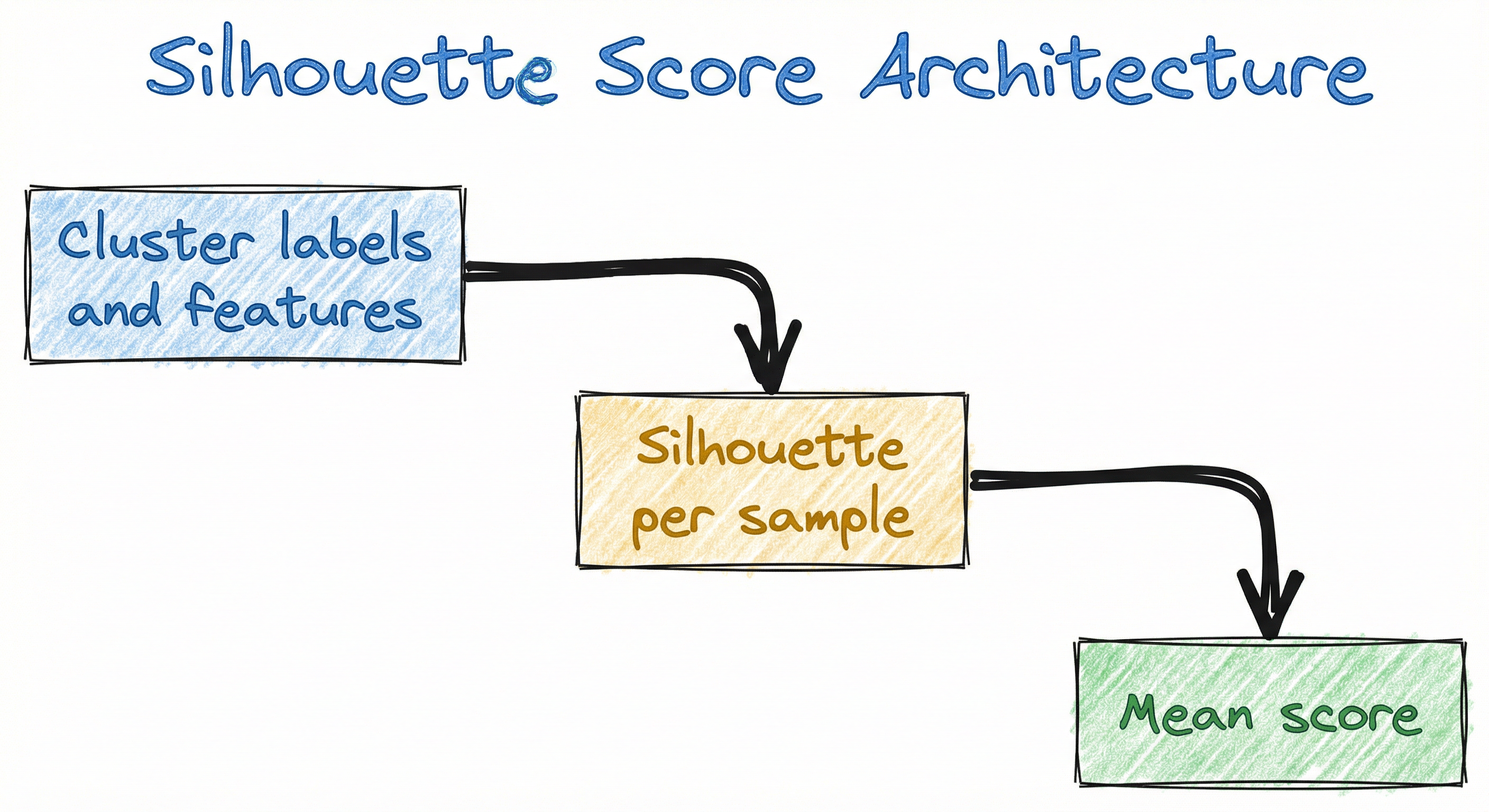
Internal Architecture

The silhouette score is computed as a post-hoc evaluation metric after clustering. The architecture involves four stages: distance computation, intra-cluster and nearest-cluster aggregation, per-sample silhouette calculation, and aggregation/visualization. Here is the data flow:

Silhouette Score in ML Systems Architecture — A directed flow from feature matrix and clustering algorithm output to pairwise distance computat...

The critical bottleneck is the pairwise distance matrix computation (Step D), which is $O(n^2)$ in both time and space. For production systems with large datasets, this is typically addressed through sampling: scikit-learn's silhouette_score accepts a sample_size parameter that randomly subsamples the data before computing distances, reducing the cost to $O(m^2)$ where $m \ll n$ .

Key Components

Distance Computer

Computes pairwise distances between all data points using the specified distance metric (Euclidean, cosine, Manhattan, etc.). This is the most expensive component at $O(n^2 \cdot d)$ . In scikit-learn, this is handled by sklearn.metrics.pairwise_distances() which supports precomputed distance matrices as input, allowing reuse across multiple K values.

Intra-Cluster Aggregator

For each sample $x_i$ in cluster $C_k$ , computes the mean distance $a(i)$ to all other members of $C_k$ . This measures cluster cohesion -- how tightly packed the cluster is around this point. Uses the precomputed distance matrix to index rows and columns belonging to the same cluster.

Nearest-Cluster Finder

For each sample $x_i$ , iterates over all other clusters $C_l$ ( $l \neq k$ ), computes the mean distance from $x_i$ to all members of $C_l$ , and selects the minimum. This identifies the nearest neighboring cluster and its distance $b(i)$ , measuring cluster separation.

Silhouette Calculator

Combines $a(i)$ and $b(i)$ via the formula $s(i) = (b(i) - a(i)) / \max(a(i), b(i))$ to produce the per-sample silhouette coefficient. Handles edge cases: singleton clusters ( $a(i) = 0, s(i) = 0$ ) and degenerate cases where $\max(a, b) = 0$ .

Aggregator & Visualizer

Aggregates per-sample silhouette values into the mean silhouette score $\bar{s}$ and per-cluster means $\bar{s}_k$ . The visualizer generates silhouette plots by sorting per-sample scores within each cluster and rendering them as horizontal bar charts with a vertical line at $\bar{s}$ for reference.

Optimal K Selector

Runs the full silhouette pipeline for multiple values of $K$ (e.g., $K = 2, 3, \ldots, 10$ ), collects mean silhouette scores, and identifies the $K$ with the highest $\bar{s}$ . Often combined with silhouette plots at each $K$ for visual validation alongside the quantitative maximum.

Data Flow

Here is the step-by-step flow for computing the silhouette score:

Step 1: Input the feature matrix $X$ of shape $(n, d)$ where $n$ is the number of samples and $d$ is the number of features.

Step 2: Run the clustering algorithm (e.g., K-Means with $K$ clusters) to produce cluster labels for each sample.

Step 3: Compute the full pairwise distance matrix $D$ of shape $(n, n)$ , where $D_{ij} = d(x_i, x_j)$ . Alternatively, if memory is constrained, compute distances on-the-fly per cluster.

Step 4: For each sample $x_i$ in cluster $C_k$ , extract the row $D[i, :]$ and partition it by cluster membership. Compute $a(i)$ as the mean of distances to same-cluster members.

Step 5: For the same sample, compute mean distances to each other cluster $C_l$ , and take the minimum to get $b(i)$ .

Step 6: Apply the silhouette formula: $s(i) = (b(i) - a(i)) / \max(a(i), b(i))$ .

Step 7: Aggregate across all samples to get the mean silhouette $\bar{s}$ .

Step 8: Repeat Steps 2-7 for multiple values of $K$ to find the optimal number of clusters.

Step 9: Generate silhouette plots for the top candidate $K$ values for visual validation.

In production, scikit-learn's silhouette_score() handles Steps 3-7 in a single call, with optional subsampling to reduce the $O(n^2)$ cost.

A directed flow from feature matrix and clustering algorithm output to pairwise distance computation, which feeds into per-sample intra-cluster distance (a) and nearest-cluster distance (b) computation, then to silhouette coefficient calculation, and finally to mean score aggregation and silhouette plot visualization for optimal K selection.

How to Implement

Computing Silhouette Score in Practice

The practical implementation of silhouette analysis revolves around two tasks: (1) computing per-sample silhouette coefficients efficiently, and (2) generating silhouette plots for visual diagnosis. The naive implementation -- computing the full $n \times n$ distance matrix and iterating over clusters -- is $O(n^2 \cdot d)$ in time and $O(n^2)$ in space. For datasets beyond ~50,000 samples, this becomes impractical without optimization.

Scikit-learn provides two key functions: silhouette_score() returns the mean silhouette, and silhouette_samples() returns per-sample values for plotting. Both accept a metric parameter supporting all scipy.spatial.distance metrics, and silhouette_score() has a sample_size parameter for subsampling large datasets.

Scaling Strategies

For production-scale datasets (100K+ samples), you have three options:

Subsampling: Use sample_size parameter in scikit-learn. A sample of 10,000-20,000 points typically gives a reliable estimate of the global mean silhouette with significantly reduced computation. Use random_state for reproducibility.
Precomputed distances: If you compute the distance matrix once, you can reuse it across multiple clustering runs with different $K$ . Pass metric='precomputed' to avoid redundant distance calculations.
Approximate methods: For truly large datasets (millions of points), use the distributed silhouette algorithm (Gaido, 2023) which achieves $O(n)$ time complexity by using cluster centroids instead of pairwise distances.

Cost Note: For a customer segmentation system at an Indian e-commerce company processing 500K customer profiles with 30 features, the full silhouette computation takes approximately 15-20 minutes on a single CPU core with 16 GB RAM. With subsampling to 10K points, this drops to under 5 seconds. On an AWS m5.4xlarge instance (INR ~30/hr or $0.36/hr), the full computation costs about INR 10 ($ 0.12). Subsampled computation is essentially free.

Basic Silhouette Score Computation with scikit-learn35 lines

from sklearn.cluster import KMeans
from sklearn.metrics import silhouette_score, silhouette_samples
from sklearn.datasets import make_blobs
import numpy as np

# Generate synthetic data with known structure
X, y_true = make_blobs(
    n_samples=500,
    n_features=2,
    centers=4,
    cluster_std=0.60,
    random_state=42
)

# Cluster with K-Means
kmeans = KMeans(n_clusters=4, random_state=42, n_init=10)
cluster_labels = kmeans.fit_predict(X)

# Compute mean silhouette score
mean_score = silhouette_score(X, cluster_labels)
print(f"Mean Silhouette Score: {mean_score:.3f}")

# Compute per-sample silhouette values
sample_scores = silhouette_samples(X, cluster_labels)

# Per-cluster analysis
for k in range(4):
    cluster_mask = cluster_labels == k
    cluster_scores = sample_scores[cluster_mask]
    print(
        f"Cluster {k}: n={cluster_mask.sum()}, "
        f"mean_silhouette={cluster_scores.mean():.3f}, "
        f"min={cluster_scores.min():.3f}, "
        f"negative_count={np.sum(cluster_scores < 0)}"
    )

This is the standard workflow for silhouette analysis. silhouette_score() returns the global mean, while silhouette_samples() gives per-sample values needed for plotting and per-cluster diagnosis. The per-cluster breakdown reveals which clusters are tight (high mean silhouette) and which have misassigned points (negative scores). Always check both the global mean and per-cluster statistics.

Optimal K Selection Using Silhouette Analysis47 lines

from sklearn.cluster import KMeans
from sklearn.metrics import silhouette_score
from sklearn.datasets import make_blobs
import matplotlib.pyplot as plt
import numpy as np

# Generate data
X, _ = make_blobs(
    n_samples=1000, n_features=5,
    centers=4, cluster_std=1.0, random_state=42
)

# Test K from 2 to 10
K_range = range(2, 11)
silhouette_scores = []
inertias = []

for k in K_range:
    kmeans = KMeans(n_clusters=k, random_state=42, n_init=10)
    labels = kmeans.fit_predict(X)
    score = silhouette_score(X, labels)
    silhouette_scores.append(score)
    inertias.append(kmeans.inertia_)
    print(f"K={k}: silhouette={score:.3f}, inertia={kmeans.inertia_:.0f}")

optimal_k = K_range[np.argmax(silhouette_scores)]
print(f"\nOptimal K by silhouette: {optimal_k}")

# Plot: Silhouette Score vs K (side-by-side with Elbow)
fig, (ax1, ax2) = plt.subplots(1, 2, figsize=(14, 5))

ax1.plot(K_range, silhouette_scores, 'bo-', linewidth=2)
ax1.axvline(x=optimal_k, color='r', linestyle='--', label=f'Optimal K={optimal_k}')
ax1.set_xlabel('Number of Clusters (K)')
ax1.set_ylabel('Mean Silhouette Score')
ax1.set_title('Silhouette Method')
ax1.legend()
ax1.grid(alpha=0.3)

ax2.plot(K_range, inertias, 'go-', linewidth=2)
ax2.set_xlabel('Number of Clusters (K)')
ax2.set_ylabel('Inertia (Within-Cluster SSE)')
ax2.set_title('Elbow Method')
ax2.grid(alpha=0.3)

plt.tight_layout()
plt.show()

This side-by-side comparison shows why the silhouette method is often preferred over the elbow method. The silhouette method has a clear maximum at the optimal K, while the elbow method requires subjective judgment about where the curve 'bends'. The silhouette method gives you a definitive answer: pick the K with the highest mean silhouette score. Note: always validate the quantitative winner with silhouette plots before committing.

Silhouette Plot Visualization for Cluster Diagnosis51 lines

from sklearn.cluster import KMeans
from sklearn.metrics import silhouette_score, silhouette_samples
from sklearn.datasets import make_blobs
import matplotlib.pyplot as plt
import matplotlib.cm as cm
import numpy as np

# Generate data
X, _ = make_blobs(n_samples=500, centers=4, cluster_std=0.6, random_state=42)

# Cluster
n_clusters = 4
kmeans = KMeans(n_clusters=n_clusters, random_state=42, n_init=10)
cluster_labels = kmeans.fit_predict(X)

# Per-sample silhouette
sample_silhouette_values = silhouette_samples(X, cluster_labels)
avg_score = silhouette_score(X, cluster_labels)

# Create silhouette plot
fig, ax = plt.subplots(1, 1, figsize=(8, 6))
y_lower = 10

for i in range(n_clusters):
    # Get silhouette values for cluster i, sorted
    ith_cluster_values = sample_silhouette_values[cluster_labels == i]
    ith_cluster_values.sort()
    size_cluster_i = ith_cluster_values.shape[0]
    y_upper = y_lower + size_cluster_i

    color = cm.nipy_spectral(float(i) / n_clusters)
    ax.fill_betweenx(
        np.arange(y_lower, y_upper),
        0, ith_cluster_values,
        facecolor=color, edgecolor=color, alpha=0.7
    )
    ax.text(-0.05, y_lower + 0.5 * size_cluster_i, str(i))
    y_lower = y_upper + 10  # padding between clusters

# Vertical line at mean silhouette score
ax.axvline(x=avg_score, color='red', linestyle='--',
           label=f'Mean silhouette = {avg_score:.3f}')

ax.set_title(f'Silhouette Plot for K={n_clusters}')
ax.set_xlabel('Silhouette Coefficient')
ax.set_ylabel('Cluster Label (sorted samples)')
ax.set_yticks([])
ax.legend(loc='best')
ax.set_xlim([-0.1, 1.0])
plt.tight_layout()
plt.show()

The silhouette plot is the most informative visualization for clustering diagnosis. Each cluster is represented by a horizontal block of sorted silhouette values. Look for: (1) roughly equal-width clusters (balanced sizes), (2) all bars extending past the red dashed mean line (all clusters above average), (3) no negative values (no misassigned points). This is adapted from scikit-learn's official silhouette analysis example and is the industry-standard approach.

Silhouette with Different Distance Metrics and Precomputed Distances38 lines

from sklearn.cluster import KMeans, AgglomerativeClustering
from sklearn.metrics import silhouette_score
from sklearn.metrics.pairwise import pairwise_distances
from sklearn.preprocessing import StandardScaler
import numpy as np

# Example: customer features (RFM-style data)
np.random.seed(42)
n_customers = 5000
X_raw = np.column_stack([
    np.random.exponential(30, n_customers),    # Recency (days)
    np.random.poisson(10, n_customers),         # Frequency
    np.random.lognormal(7, 1.5, n_customers),   # Monetary (INR)
])

# ALWAYS scale features before silhouette analysis
scaler = StandardScaler()
X = scaler.fit_transform(X_raw)

# Compare distance metrics
for metric in ['euclidean', 'cosine', 'manhattan']:
    # Precompute distance matrix (reusable across K values)
    D = pairwise_distances(X, metric=metric)

    scores = {}
    for k in [3, 4, 5, 6]:
        kmeans = KMeans(n_clusters=k, random_state=42, n_init=10)
        labels = kmeans.fit_predict(X)
        # Use precomputed distances
        score = silhouette_score(D, labels, metric='precomputed')
        scores[k] = score

    best_k = max(scores, key=scores.get)
    print(
        f"Metric: {metric:12s} | Best K={best_k} "
        f"(score={scores[best_k]:.3f}) | "
        f"All: {', '.join(f'K={k}:{v:.3f}' for k, v in scores.items())}"
    )

Two critical practices demonstrated here: (1) Feature scaling -- the silhouette score uses distances, so unscaled features with different ranges will dominate the distance calculation. Always standardize before computing silhouette. (2) Precomputed distances -- when testing multiple K values, compute the distance matrix once and reuse it via metric='precomputed'. This saves significant computation. The example also shows how the optimal K and score can vary across distance metrics, so always try multiple metrics for your data.

Subsampled Silhouette for Large Datasets42 lines

from sklearn.cluster import MiniBatchKMeans
from sklearn.metrics import silhouette_score
import numpy as np
import time

# Simulate large dataset (e.g., 500K e-commerce customers)
np.random.seed(42)
n_samples = 500_000
n_features = 30
X_large = np.random.randn(n_samples, n_features)

# Cluster with MiniBatchKMeans for speed
kmeans = MiniBatchKMeans(n_clusters=8, random_state=42, batch_size=10000)
labels = kmeans.fit_predict(X_large)

# Full silhouette (WARNING: very expensive)
# Estimated time: ~15-20 minutes, ~186 GB RAM for distance matrix
# DON'T do this: silhouette_score(X_large, labels)

# Subsampled silhouette (recommended for n > 50K)
for sample_size in [5000, 10000, 20000, 50000]:
    scores = []
    for trial in range(5):
        start = time.time()
        score = silhouette_score(
            X_large, labels,
            sample_size=sample_size,
            random_state=trial  # different seed per trial
        )
        elapsed = time.time() - start
        scores.append(score)

    mean_score = np.mean(scores)
    std_score = np.std(scores)
    print(
        f"sample_size={sample_size:6d} | "
        f"mean={mean_score:.4f} +/- {std_score:.4f} | "
        f"time={elapsed:.2f}s"
    )

# Production recommendation:
# Use sample_size=10000-20000, run 5 trials, report mean +/- std

For large datasets, the full silhouette computation is impractical ( $O(n^2)$ memory and time). The sample_size parameter in scikit-learn randomly subsamples the data before computing. With 10K-20K samples, you get a reliable estimate in seconds instead of hours. Running multiple trials with different random seeds gives you a confidence interval. This is the standard production approach at companies processing millions of data points for customer segmentation.

Configuration Example23 lines

# scikit-learn silhouette_score configuration examples

from sklearn.metrics import silhouette_score, silhouette_samples

# Basic usage (Euclidean distance, no subsampling)
score = silhouette_score(X, labels)

# Cosine distance (for text/NLP embeddings)
score = silhouette_score(X, labels, metric='cosine')

# Manhattan distance
score = silhouette_score(X, labels, metric='manhattan')

# Subsampled for large datasets
score = silhouette_score(X, labels, sample_size=10000, random_state=42)

# Precomputed distance matrix (reusable across K values)
from sklearn.metrics.pairwise import pairwise_distances
D = pairwise_distances(X, metric='euclidean')
score = silhouette_score(D, labels, metric='precomputed')

# Per-sample values for silhouette plot
per_sample = silhouette_samples(X, labels, metric='euclidean')

Common Implementation Mistakes

●
Forgetting to scale features before computing silhouette. The silhouette score relies on distances, so features with larger ranges dominate. Customer monetary value in INR (thousands) will overwhelm purchase frequency (single digits). Always use StandardScaler or MinMaxScaler before clustering and silhouette computation.
●
Using silhouette score with non-globular cluster shapes. The silhouette coefficient assumes convex, roughly spherical clusters. For crescent-shaped, ring-shaped, or elongated clusters (common in DBSCAN output), silhouette will penalize correct clusterings. Use DBCV (Density-Based Clustering Validation) instead.
●
Computing full silhouette on datasets larger than 50K samples without subsampling. The $O(n^2)$ cost means 100K samples requires ~74 GB RAM for the distance matrix (float64). Always use sample_size parameter or precompute on a subsample. A 10K subsample gives a reliable estimate in seconds.
●
Only looking at the mean silhouette score and ignoring the per-sample distribution. A mean of 0.55 could hide one excellent cluster (mean 0.85) and one terrible cluster (mean 0.25). Always generate silhouette plots to diagnose individual clusters.
●
Using silhouette to evaluate clusterings with K=1. The silhouette score is undefined for a single cluster (there is no neighboring cluster to compare against). It requires $K \geq 2$ .
●
Applying silhouette score to high-dimensional data without dimensionality reduction. In high dimensions, distances converge (curse of dimensionality), making all silhouette scores cluster near zero regardless of true cluster quality. Apply PCA, t-SNE, or UMAP before evaluating.

When Should You Use This?

Use When

You need an internal validation metric for clustering when no ground truth labels are available -- the most common real-world scenario for unsupervised learning
You want to select the optimal number of clusters K with a clear, quantitative criterion (maximum mean silhouette) rather than the subjective elbow method
You need per-sample diagnostic information to identify misassigned points, boundary cases, and problematic clusters -- not just a global quality score
Your clusters are expected to be roughly convex and globular (e.g., K-Means, Gaussian Mixture Models) where distance-based cohesion/separation measures are meaningful
You are working with moderate-sized datasets (under 50K samples) where the $O(n^2)$ cost is acceptable, or you can subsample larger datasets for an approximate score
You want a metric that works with any distance metric (Euclidean, cosine, Manhattan, etc.) and is not tied to a specific clustering algorithm

Avoid When

Your clusters have non-convex shapes (crescents, rings, nested clusters) -- silhouette penalizes correct DBSCAN-style clusterings because points near elongated cluster boundaries have high intra-cluster distances
Your dataset has millions of samples and you cannot afford even subsampled computation -- use the Davies-Bouldin Index ( $O(n \cdot K)$ ) or Calinski-Harabasz Index instead
You have ground truth labels available -- use external metrics like ARI (Adjusted Rand Index) or NMI (Normalized Mutual Information) which directly measure agreement with the known partition
Your data is very high-dimensional (hundreds or thousands of features) without dimensionality reduction -- distance metrics degenerate in high dimensions, making silhouette scores meaningless
You are evaluating density-based clustering (DBSCAN, HDBSCAN) where cluster shapes are arbitrary -- use DBCV (Density-Based Cluster Validation) instead, which respects density-connected components
Your clusters have highly unequal sizes -- silhouette tends to favor balanced cluster sizes and can give misleading scores when one cluster is 100x larger than another

Key Tradeoffs

Silhouette vs. Elbow Method

The elbow method plots within-cluster sum of squares (inertia) against K and looks for the "bend." The silhouette method plots mean silhouette score against K and picks the maximum. The key trade-off:

Aspect	Elbow Method	Silhouette Method
Criterion	Subjective (find the bend)	Objective (maximum score)
Computation	$O(n \cdot K \cdot d)$ per K	$O(n^2 \cdot d)$ per K
Per-sample insight	No	Yes (silhouette plot)
Interpretability	Moderate	High ([-1, +1] range)
Cluster shape bias	Convex only	Convex only

In practice, use both together. The elbow method is cheap and gives a rough range; the silhouette method confirms the optimal K within that range and provides diagnostic plots.

Silhouette vs. Davies-Bouldin Index

The Davies-Bouldin (DB) Index computes the maximum ratio of intra-cluster scatter to inter-cluster distance for each cluster pair, then averages. Lower is better (opposite of silhouette). The key trade-off: DB is $O(n \cdot K)$ -- orders of magnitude faster for large datasets -- but uses centroids instead of pairwise distances, losing per-sample granularity. Use DB for quick screening, silhouette for detailed analysis.

Silhouette vs. Calinski-Harabasz Index

The Calinski-Harabasz (CH) Index measures the ratio of between-cluster variance to within-cluster variance. Higher is better. Like DB, it is $O(n \cdot K)$ and uses centroids. CH tends to favor well-separated, compact clusters (like silhouette) but provides no per-sample breakdown. It is unbounded (no [-1, +1] range), making absolute values less interpretable across datasets.

The Shape Bias Problem

All three internal metrics (silhouette, DB, CH) share a fundamental bias: they assume convex, globular clusters. For non-convex structures, they will incorrectly penalize valid density-based clusterings. If your data has complex shapes, consider DBCV or visual inspection of t-SNE/UMAP embeddings.

Rule of Thumb: Use silhouette analysis as your primary internal validation tool when cluster shapes are roughly convex, dataset size is manageable (<50K or with subsampling), and you need per-sample diagnostics. Complement with the elbow method for a quick sanity check and Davies-Bouldin for large-scale screening.

Alternatives & Comparisons

Davies-Bouldin Index

The Davies-Bouldin (DB) Index uses cluster centroids to measure the ratio of intra-cluster scatter to inter-cluster separation, with lower values indicating better clustering. Its major advantage over silhouette is computational efficiency: $O(n \cdot K)$ vs. $O(n^2)$ , making it practical for large datasets where silhouette is infeasible. However, DB lacks per-sample granularity -- you get one score per cluster pair, not per data point. Choose DB for quick, large-scale screening; choose silhouette when you need detailed per-sample diagnosis and can afford the quadratic cost.

Calinski-Harabasz Index

The Calinski-Harabasz (CH) Index, also called the Variance Ratio Criterion, measures the ratio of between-cluster dispersion to within-cluster dispersion. Higher values indicate better clustering. Like Davies-Bouldin, it is $O(n \cdot K)$ and centroid-based, making it far faster than silhouette for large datasets. However, it has no bounded range (unlike silhouette's [-1, +1]), making absolute scores harder to interpret across datasets. The CH Index also lacks per-sample scores. Use CH alongside silhouette for a complementary perspective -- they sometimes disagree on optimal K.

ARI / NMI (Adjusted Rand Index / Normalized Mutual Information)

ARI and NMI are external validation metrics that require ground truth cluster labels to evaluate. They measure how well the predicted clustering agrees with the true partition. ARI is chance-adjusted (0 for random, 1 for perfect); NMI uses information-theoretic principles (0 to 1). When you have ground truth, ARI/NMI are strictly superior to silhouette because they directly measure what you care about. Use silhouette only when no ground truth exists -- which is the typical production scenario for unsupervised clustering.

Confusion Matrix (for supervised clustering evaluation)

When ground truth labels are available, you can construct a confusion matrix between predicted clusters and true classes (via optimal matching). This gives raw counts of correct and incorrect assignments. Unlike silhouette, it requires ground truth and is a supervised metric. Use it for validating clustering algorithms on labeled benchmarks; use silhouette for real-world unsupervised evaluation where no labels exist.

Pros, Cons & Tradeoffs

Advantages

No ground truth required (internal validation) -- works in the most common real-world scenario where you have no labeled clusters, making it the go-to metric for production unsupervised learning pipelines.
Per-sample granularity via silhouette plots provides far richer diagnostic information than global-only metrics. You can identify specific misassigned points, boundary cases, and problematic clusters -- not just a single quality number.
Interpretable bounded range [-1, +1] with clear semantics: +1 is perfect, 0 is boundary, -1 is misassigned. This makes it easy to communicate clustering quality to non-technical stakeholders and set quality thresholds.
Distance-metric agnostic -- works with Euclidean, cosine, Manhattan, or any custom distance function. This flexibility means it adapts to the data domain (e.g., cosine for text embeddings, Euclidean for numeric features).
Objective K selection -- unlike the subjective elbow method, the silhouette method provides a clear criterion: pick K with the highest mean silhouette score. No ambiguous "bends" to interpret.
Widely implemented in all major ML libraries (scikit-learn, R cluster package, MATLAB, Spark MLlib) with battle-tested implementations handling edge cases correctly.

Disadvantages

$O(n^2)$ computational cost is the primary limitation. For 100K samples, the distance matrix requires ~74 GB RAM. Subsampling mitigates this but introduces approximation error and requires multiple trials for stability.
Biased toward convex, globular clusters of similar size. Non-convex cluster shapes (crescents, rings), density-based clusters (DBSCAN output), and highly imbalanced cluster sizes receive artificially low silhouette scores.
Degrades in high dimensions due to the curse of dimensionality -- distances converge in high-dimensional spaces, making all silhouette scores cluster near zero regardless of actual cluster quality. Dimensionality reduction is a prerequisite.
Not defined for K=1 -- you cannot evaluate whether the data should be treated as a single cluster versus multiple clusters. You need K >= 2, so it cannot help with the fundamental question "should I cluster at all?"
Sensitive to outliers -- a single outlier far from all clusters can have a very negative silhouette score, dragging down the global mean and making a good clustering look mediocre. Outlier detection should precede silhouette analysis.
No probabilistic interpretation -- unlike BIC/AIC for mixture models, the silhouette score has no information-theoretic or Bayesian grounding. A score of 0.6 vs 0.55 is "better" but you cannot quantify statistical significance without bootstrapping.

Establish a null distribution by computing silhouette scores on permuted or random data with the same shape. If the real silhouette score is not significantly higher than the null, the clusters are meaningless. The Gap Statistic formalizes this approach by comparing the within-cluster dispersion to that expected under a null reference distribution.

Placement in an ML System

Where Does Silhouette Score Fit in the ML Pipeline?

Silhouette analysis lives in the evaluation and model selection phase of unsupervised learning pipelines. Here is the typical workflow:

During Feature Engineering: You prepare the feature matrix, apply scaling (StandardScaler), and optionally reduce dimensionality (PCA to retain 95% variance). The silhouette score will be computed on this preprocessed data -- never on raw, unscaled features.

During Clustering: Run your clustering algorithm (K-Means, agglomerative, DBSCAN) with candidate hyperparameters. For K-Means, this typically means testing $K = 2$ through $K = 10$ or more.

Evaluation Phase: For each candidate clustering, compute the silhouette score. If $n < 50K$ , use the full dataset. If $n > 50K$ , subsample to 10K-20K points. Select the configuration with the highest mean silhouette score, then validate with silhouette plots.

Post-Evaluation: Once the optimal clustering is selected, use the per-sample silhouette scores to identify boundary points (score near 0) and misassigned points (negative score). These points may need manual review or special handling in downstream tasks.

In Production: For recurring clustering tasks (e.g., monthly customer re-segmentation), establish a baseline silhouette score. Monitor it over time -- a significant drop (e.g., from 0.55 to 0.40) indicates data distribution shift or degraded cluster quality, triggering re-tuning.

Key Insight: Silhouette analysis is an offline evaluation metric, not a runtime metric. It guides cluster count selection and quality validation during model development. In production, it serves as a monitoring signal for cluster quality degradation, not a per-request computation.

Pipeline Stage

Evaluation / Model Selection

Upstream

Feature Engineering
Dimensionality Reduction (PCA/UMAP)
Clustering Algorithm (K-Means, DBSCAN, etc.)

Downstream

Optimal K Selection
Cluster Interpretation & Labeling
Downstream Task (Recommendation, Segmentation, Anomaly Detection)

Scaling Bottlenecks

Where Silhouette Score Gets Expensive

The core bottleneck is the $O(n^2 \cdot d)$ pairwise distance computation:

1. Single Evaluation: For $n = 10{,}000$ samples with $d = 50$ features, silhouette takes ~2 seconds on a modern CPU. For $n = 50{,}000$ , it takes ~1 minute. For $n = 100{,}000$ , the distance matrix alone needs ~74 GB RAM (float64), making it infeasible on most machines without subsampling.

2. K Sweep: Testing $K = 2, 3, \ldots, 10$ means 9 clustering runs plus 9 silhouette computations. If you precompute the distance matrix once and reuse it, the total is ~ $O(n^2 \cdot d) + 9 \times O(n^2)$ . Without precomputation, it is $9 \times O(n^2 \cdot d)$ .

3. Hyperparameter Tuning: Grid search over clustering parameters (K, initialization method, distance metric) with silhouette evaluation can multiply the cost by 50-100x. For $n = 50K$ , this means 50-100 minutes of pure evaluation time.

4. Distributed Systems: The distributed silhouette algorithm (Gaido, 2023) reduces to $O(n)$ time using centroid-based approximations, but requires Spark or similar distributed frameworks. Viable for $n > 1M$ on cluster infrastructure.

For most production systems, the recommendation is: cluster on the full dataset, evaluate silhouette on a 10K-20K subsample, and validate the winner with a silhouette plot. This reduces cost from hours to seconds with negligible loss of accuracy.

Production Case Studies

E-Commerce Customer Segmentation (India)Retail & E-Commerce

Customer segmentation is one of the most common applications of clustering in Indian e-commerce. Companies like Flipkart, Myntra, and BigBasket segment millions of customers using RFM (Recency, Frequency, Monetary) features. The standard workflow involves scaling RFM features with StandardScaler, running K-Means for K=2 through K=10, and selecting the optimal K using silhouette analysis. A typical Indian e-commerce dataset with 500K customers and 30 behavioral features is subsampled to 15K points for silhouette evaluation. The silhouette plot reveals whether segments like "High-Value Frequent Buyers" (high monetary, high frequency) are well-separated from "Bargain Hunters" (low monetary, high frequency) and "Dormant Users" (high recency, low frequency).

Outcome:

Using silhouette analysis, teams typically converge on K=4 to K=6 customer segments with mean silhouette scores of 0.45-0.65. This translates to actionable segments for personalized marketing campaigns. A well-segmented campaign at a mid-size Indian e-commerce company (GMV ~INR 500 Cr or ~ $60M) can improve conversion rates by 15-25% through targeted offers, translating to INR 5-10 Cr (~$ 600K-$1.2M) additional annual revenue.

Spotify / Music Content ClusteringEntertainment & Media

Music streaming platforms like Spotify use audio feature clustering to group songs by characteristics such as tempo, energy, danceability, acousticness, and valence. Clustering song catalogs with K-Means and evaluating with silhouette analysis helps build content-based recommendation systems. A clustering study on Spotify audio features found that the highest silhouette score was for K=2 (0.25), with K=3, 4, and 8 also showing strong scores (~0.238-0.241). The relatively low absolute scores reflect the inherent overlap in musical features -- songs often blend genres and moods.

Outcome:

Even with modest silhouette scores (0.20-0.25), the clusters provide meaningful groupings for recommendation engines. The silhouette analysis reveals which song features contribute most to cluster separation, guiding feature engineering for collaborative filtering models. In India, platforms like JioSaavn and Gaana use similar approaches to cluster their catalogs of 100M+ songs across Hindi, Tamil, Telugu, and other regional languages.

Medical Image & Patient ClusteringHealthcare

Hospitals and research institutions use clustering for patient stratification and medical image segmentation. At institutions like AIIMS and Apollo Hospitals, patient cohorts are clustered based on clinical features (lab values, vital signs, treatment history) to identify subgroups with different treatment responses. The silhouette score validates whether the identified subgroups are genuinely distinct. In radiology, K-Means clustering of pixel intensities for tissue segmentation uses silhouette analysis to determine the optimal number of tissue classes (e.g., white matter, gray matter, CSF in brain MRI).

Outcome:

Patient stratification studies typically achieve silhouette scores of 0.35-0.55, reflecting the inherent complexity of medical data. The per-cluster silhouette breakdown identifies which patient subgroups are well-defined (e.g., clearly distinct treatment responders) and which overlap (e.g., intermediate-risk patients). This informs clinical trial design by highlighting which cohorts can be reliably separated for targeted treatments.

Netflix / Content Recommendation ClusteringEntertainment & Streaming

Netflix's content catalog is clustered using features like genre, cast, director, description embeddings (TF-IDF), and release year to power content-based recommendations. An analysis of Netflix's 2019 catalog applied K-Means, Agglomerative Clustering, and DBSCAN, evaluating each with silhouette scores. The study used TF-IDF vectors of content descriptions (high-dimensional) combined with PCA for dimensionality reduction before silhouette computation. The silhouette analysis identified the optimal K and compared algorithm performance.

Outcome:

Agglomerative clustering with K=7 achieved the best silhouette score among the algorithms tested. The silhouette plots revealed that content clusters for niche genres (documentaries, stand-up comedy) had high cohesion, while broad genres (drama, thriller) had lower scores due to internal diversity. In India, Hotstar (Disney+) applies similar methods to cluster content across 10+ languages, where silhouette analysis helps validate that language-specific content groupings are genuinely separated.

Tooling & Ecosystem

scikit-learn (Python)

PythonOpen Source

The de facto standard for silhouette analysis in Python. Provides silhouette_score() for the global mean and silhouette_samples() for per-sample values. Supports all scipy.spatial.distance metrics, precomputed distance matrices, and subsampling via the sample_size parameter. Also includes an official tutorial on silhouette analysis for K-Means clustering with complete plotting code.

Yellowbrick (Python)

PythonOpen Source

A machine learning visualization library built on scikit-learn. The SilhouetteVisualizer generates publication-quality silhouette plots with a single API call. Automatically color-codes clusters, adds the mean silhouette line, and handles all layout details. The quickest way to generate silhouette plots: SilhouetteVisualizer(KMeans(5)).fit(X).show().

R cluster package

ROpen Source

The cluster package in R provides silhouette() for computing per-sample silhouette values and built-in plotting methods. It supports any dissimilarity matrix and integrates with R's base plotting system. The fpc package extends this with the cluster.stats() function that computes silhouette alongside 30+ other clustering validation measures.

Apache Spark MLlib

Scala / Python / JavaOpen Source

Spark's ClusteringEvaluator computes silhouette scores in a distributed setting, enabling evaluation on datasets with millions of records across a cluster. Supports the squared Euclidean and cosine distance metrics. Essential for big data clustering pipelines at companies processing petabyte-scale data on AWS EMR or Databricks (cloud cost: ~INR 500-2000/hr or ~$6-24/hr for a 10-node cluster).

MATLAB Statistics and Machine Learning Toolbox

MATLABCommercial

The evalclusters() function in MATLAB computes the silhouette criterion (among others) for optimal K selection. Also provides silhouette() for per-sample plots. Widely used in academic research, biomedical engineering, and industrial applications. Commercial license required (academic pricing: ~INR 6,000 or ~$72/year for students).

PyClustering

Python / C++Open Source

An open-source Python/C++ library for clustering algorithms and validation. Implements silhouette analysis alongside many clustering algorithms not available in scikit-learn (BIRCH, CURE, ROCK, etc.). The C++ core provides faster computation than pure Python implementations for moderate-sized datasets.

Research & References

Silhouettes: A Graphical Aid to the Interpretation and Validation of Cluster Analysis

Rousseeuw, Peter J. (1987)Journal of Computational and Applied Mathematics

The foundational paper introducing the silhouette coefficient and silhouette plot. Proposes the $(b-a)/\max(a,b)$ formula for per-sample cluster validation and demonstrates its use with several real datasets. Has over 18,000 citations and remains the canonical reference for silhouette analysis.

Scalable Distributed Approximation of Internal Measures for Clustering Evaluation

Ceccarello, Pietracaprina & Pucci (2020)arXiv preprint

Presents the first provably accurate scalable algorithm for approximating the silhouette coefficient on massive datasets. Uses a Probability Proportional to Size (PPS) sampling scheme to approximate the silhouette within additive error $O(\epsilon)$ with high probability, using a small number of distance calculations -- addressing the $O(n^2)$ bottleneck.

Distributed Silhouette Algorithm: Evaluating Clustering on Big Data

Gaido, Marco (2023)arXiv preprint

Achieves silhouette computation with linear $O(n)$ time complexity by using centroid-based approximations. Implemented for squared Euclidean and cosine distances. Enables silhouette evaluation on billion-scale datasets in distributed Spark environments, though it sacrifices per-sample exact values for scalability.

Deep Clustering Using the Soft Silhouette Score: Towards Compact and Well-Separated Clusters

Vardakas, Papakostas, et al. (2024)arXiv preprint

Introduces a differentiable soft silhouette score that can be used as a training objective for deep clustering models. Instead of hard cluster assignments, it uses soft assignments from neural networks, enabling end-to-end optimization of both feature representations and cluster quality simultaneously.

Revisiting Silhouette Aggregation

Buono & Ferraro (2024)arXiv preprint

Proposes per-cluster sampling strategies that are considerably more robust than standard uniform sampling for approximating the silhouette score. Shows that per-cluster sampling yields approximately the same score even when the subsampled space is only 2% of the original data, providing dramatic speedups with minimal accuracy loss.

When Does the Silhouette Score Work?

Various authors (2024)arXiv preprint

Provides a rigorous analysis of when the silhouette score correctly identifies the true number of clusters. Identifies conditions under which silhouette fails (non-convex clusters, high dimensionality, unequal cluster densities) and proposes practical guidelines for practitioners on when to trust silhouette analysis versus alternative metrics.

Interview & Evaluation Perspective

Common Interview Questions

●
Explain the silhouette score to a product manager. What does a score of 0.6 mean in practical terms?
●
Walk me through how you would select the optimal number of clusters K for a customer segmentation task using silhouette analysis.
●
The silhouette score for your clustering is 0.25. Is that good or bad? What would you do next?
●
Why is the silhouette score computationally expensive, and how would you handle a dataset with 1 million samples?
●
Compare silhouette score, Davies-Bouldin Index, and Calinski-Harabasz Index. When would you use each?
●
Your DBSCAN clustering looks correct visually, but the silhouette score is low. What is happening?

Key Points to Mention

●
The silhouette coefficient formula is $(b-a)/\max(a,b)$ where $a$ is mean intra-cluster distance and $b$ is mean nearest-cluster distance. Range is [-1, +1]. This captures both cluster cohesion (small $a$ ) and separation (large $b$ ) in a single metric.
●
The silhouette plot (sorted per-sample bars grouped by cluster) is more diagnostic than the mean score alone. It reveals cluster size imbalance, misassigned points (negative bars), and boundary cases (bars near zero). Always plot it before making K decisions.
●
The $O(n^2)$ computational cost is the primary practical limitation. For large datasets, use subsampling (10K-20K points) or switch to $O(n \cdot K)$ alternatives like Davies-Bouldin or Calinski-Harabasz for initial screening.
●
Silhouette assumes convex, globular clusters. It gives misleadingly low scores for non-convex shapes (DBSCAN output). For density-based clustering, use DBCV (Density-Based Cluster Validation) instead.
●
Always scale features before computing silhouette. Unscaled features with different ranges will dominate the distance calculation. StandardScaler is the standard preprocessing step.
●
Silhouette tends to favor fewer clusters (K=2 often wins). Combine with domain knowledge to constrain the K range and use silhouette plots to validate structure at higher K values.

Pitfalls to Avoid

●
Claiming silhouette is the only clustering metric you need. A senior candidate should mention it alongside Davies-Bouldin, Calinski-Harabasz, Gap Statistic, and external metrics (ARI, NMI) when ground truth exists.
●
Forgetting the $O(n^2)$ cost and proposing to compute silhouette on millions of samples without discussing subsampling or approximation strategies.
●
Using silhouette to evaluate DBSCAN or other density-based algorithms without acknowledging the convex-cluster bias. This is a common trap interviewers set.
●
Reporting only the mean silhouette score without mentioning silhouette plots and per-cluster analysis. The per-sample perspective is what distinguishes silhouette from other metrics.
●
Not mentioning feature scaling. If a candidate computes silhouette on unscaled RFM data, the result is meaningless because monetary value dominates.

Senior-Level Expectation

A senior candidate should articulate the per-sample formula and its geometric intuition (cohesion vs. separation), explain the silhouette plot as the primary diagnostic tool (not just the mean), and discuss computational scaling strategies for production datasets (subsampling, precomputed distances, distributed approximation). They should compare silhouette with Davies-Bouldin and Calinski-Harabasz, explaining the trade-off between per-sample granularity and $O(n \cdot K)$ speed. For system design, they should describe an end-to-end clustering pipeline: scale features, reduce dimensions if needed, run K-Means for K=2-10, evaluate with silhouette, validate with plots, and monitor silhouette over time for drift. The strongest candidates will mention the convex cluster bias, propose DBCV for density-based clustering, and discuss the null distribution approach (Gap Statistic) for determining whether clustering is meaningful at all. Quantifying impact is key: 'A 0.15 improvement in silhouette score from 0.40 to 0.55 in customer segmentation at a company with 10M users and INR 500 Cr GMV can mean the difference between 4 vague segments and 6 actionable ones, enabling targeted campaigns worth INR 5-8 Cr in incremental revenue.'

Summary

Let us bring everything together.

The Silhouette Score is an internal cluster validation metric that measures two essential properties of a good clustering: cohesion (how close each point is to its own cluster) and separation (how far each point is from the nearest alternative cluster). The per-sample formula $s(i) = (b(i) - a(i)) / \max(a(i), b(i))$ produces a value in $[-1, +1]$ , where +1 indicates perfect cluster assignment, 0 indicates a boundary point, and -1 indicates likely misassignment. The mean silhouette across all samples gives an overall clustering quality score, and the silhouette plot -- sorted per-sample bars grouped by cluster -- provides the richest diagnostic visualization available for unsupervised learning.

When to use it: The silhouette score excels when you need a label-free metric with per-sample granularity, when cluster shapes are roughly convex (K-Means, GMM), and when dataset size is manageable ( $n < 50K$ or with subsampling). It provides an objective criterion for optimal K selection (pick the K with the highest mean silhouette), eliminating the subjectivity of the elbow method. It is implemented in all major ML libraries and is the standard first-line metric for production clustering evaluation in customer segmentation, content grouping, and anomaly detection.

When to be cautious: The $O(n^2)$ computational cost is the primary practical limitation -- always subsample for datasets beyond 50K points. The metric is biased toward convex, globular clusters of similar size, making it inappropriate for density-based clustering output (use DBCV instead). It degrades in high dimensions due to distance convergence and is not defined for $K = 1$ . Always complement silhouette with domain knowledge, visual inspection (t-SNE/UMAP plots), and alternative metrics (Davies-Bouldin for large-scale screening, ARI/NMI when ground truth is available).

Key technical points: (1) Always scale features before computing silhouette. (2) Use silhouette plots, not just the mean score, for diagnostic insight. (3) For large datasets, subsample to 10K-20K points or use precomputed distances. (4) Combine with the elbow method: use elbow for cheap range narrowing, silhouette for final selection. (5) Watch for the "K=2 bias" -- silhouette often favors fewer clusters, so constrain the range with domain knowledge. (6) Recent advances in distributed (Gaido, 2023) and soft silhouette (Vardakas et al., 2024) are extending its applicability to big data and deep learning.

Final Insight: The silhouette score is the single most informative internal clustering metric because it provides per-sample granularity that no alternative matches. But a score is only as good as the assumptions behind it. Understand when convex-cluster assumptions hold, manage computational costs through sampling, and always pair the quantitative score with visual validation. That combination -- silhouette analysis plus domain judgment -- is what turns clustering from an art into an engineering discipline.

Concept Snapshot

Why This Concept Exists

The Fundamental Problem: No Labels, No Loss Function

Before Silhouette: The Wild West of Cluster Validation

Rousseeuw's Insight: Per-Sample Cluster Fit

Evolution and Modern Usage

Core Intuition & Mental Model

The Coffee Shop Analogy

The Silhouette Plot: An X-Ray of Your Clustering

Mental Model for Practitioners

Technical Foundations

Per-Sample Silhouette Coefficient

Properties of the Silhouette Coefficient

Mean Silhouette Score

Per-Cluster Mean Silhouette

Computational Complexity

Relationship to Other Internal Indices

Internal Architecture

Key Components

Data Flow

How to Implement

Computing Silhouette Score in Practice

Scaling Strategies

Common Implementation Mistakes

When Should You Use This?

Use When

Avoid When

Key Tradeoffs

Silhouette vs. Elbow Method

Silhouette vs. Davies-Bouldin Index

Silhouette vs. Calinski-Harabasz Index

The Shape Bias Problem

Alternatives & Comparisons

Pros, Cons & Tradeoffs

Advantages

Disadvantages

Failure Modes & Debugging

False Low Score on Non-Convex Clusters

Memory Crash on Large Datasets

Misleading High Score Due to Feature Dominance

Score Degrades to Zero in High Dimensions

Optimal K Favors Too Few Clusters

Silhouette Overestimates Quality with Balanced Random Data

Placement in an ML System

Where Does Silhouette Score Fit in the ML Pipeline?

Pipeline Stage

Upstream

Downstream

Scaling Bottlenecks

Production Case Studies

Tooling & Ecosystem

Research & References

Interview & Evaluation Perspective

Common Interview Questions

Key Points to Mention

Pitfalls to Avoid

Senior-Level Expectation

Summary

Related Blocks & Further Reading

Related ML Blocks

Further Reading