NDCG in Machine Learning
Let's start with the fundamental question: how do you know if your search engine or recommendation system is actually good?
You could count how many relevant items you returned -- but that ignores order. A search result with the perfect answer buried at position 47 is pretty much worthless, even if technically it "contains" the relevant document.
You could check if the top result is relevant -- but that ignores everything else. A recommendation list with one great item and nine terrible ones isn't much better than random.
This is exactly the problem NDCG (Normalized Discounted Cumulative Gain) solves. It's a ranking evaluation metric that answers the question: "How good is this ordered list?" by accounting for both relevance and position.
NDCG measures ranking quality using two core insights: (1) more relevant items are worth more than less relevant ones (graded relevance), and (2) relevant items at the top are worth exponentially more than relevant items lower down (position discount). It normalizes the score against an ideal ranking, giving you a number between 0 and 1 that tells you exactly how close your ranking is to perfection.
Today, NDCG is the de facto standard for evaluating search engines, recommendation systems, and any ML system that produces ranked lists. Google uses it internally to measure search quality. Amazon uses it to evaluate product ranking. Netflix uses it to assess recommendation carousels. From Flipkart's product search to Swiggy's restaurant recommendations -- if you're ranking things by relevance, you're almost certainly measuring it with NDCG.
Concept Snapshot
- What It Is
- A position-aware ranking evaluation metric that measures how well a ranked list matches an ideal ordering by assigning graded relevance scores, discounting them by logarithmic position, and normalizing against the best possible ranking.
- Category
- Evaluation
- Complexity
- Intermediate
- Inputs / Outputs
- Inputs: a ranked list of items and their ground-truth relevance scores (typically 0-4 scale). Outputs: a single score between 0 and 1, where 1 represents perfect ranking.
- System Placement
- Used offline during model evaluation and online for A/B testing of ranking algorithms in search engines, recommendation systems, and retrieval pipelines.
- Also Known As
- Normalized DCG, nDCG, NDCG@K, Normalized Discounted Cumulative Gain
- Typical Users
- ML engineers, search engineers, ranking specialists, recommendation system developers, IR researchers
- Prerequisites
- Basic ranking concepts, Ground-truth relevance labels, Logarithms, Information retrieval fundamentals
- Key Terms
- DCGIDCGposition discountgraded relevanceNDCG@Klog2 discountcumulative gainranking quality
Why This Concept Exists
The Problem with Binary Relevance Metrics
Early information retrieval metrics like precision and recall treated relevance as binary: a document is either relevant or not. But real-world relevance isn't binary. When you search for "best restaurants in Mumbai," the result might be:
- Perfectly relevant: a 2024 guide to top-rated Mumbai restaurants
- Somewhat relevant: a general India food guide that mentions Mumbai
- Barely relevant: an article about Indian cuisine with one Mumbai reference
- Irrelevant: a restaurant in Mumbai, Ohio
Binary metrics can't capture these gradations. They'd count all four as equally "relevant" or "irrelevant," losing critical information about ranking quality.
The Problem with Position-Unaware Metrics
Even graded relevance metrics like precision@K fail to account for position. Consider two search results for "Python tutorial":
Ranking A: [Perfect, Good, Good, Mediocre, Irrelevant] Ranking B: [Irrelevant, Mediocre, Good, Good, Perfect]
Both have the same precision@5 and the same distribution of relevance scores. But Ranking A is obviously superior -- users see the best content immediately. Position-unaware metrics can't distinguish them.
The User Behavior Reality
Eye-tracking studies on search behavior consistently show that users scan results from top to bottom, with attention dropping exponentially. The probability a user clicks on position 1 is roughly 10x higher than position 10. A metric that ignores position ignores how humans actually use ranked lists.
The Birth of DCG and NDCG
In 2000, Kalervo Järvelin and Jaana Kekäläinen at the University of Tampere faced exactly this problem while evaluating IR systems. They introduced Cumulated Gain-based evaluation in their seminal 2002 ACM TOIS paper "Cumulated Gain-Based Evaluation of IR Techniques."
Their insight: discount relevance scores by a logarithmic function of position, then sum them up. Documents at position 1 get full credit. Position 2 gets discounted by log₂(3) ≈ 0.63. Position 10 gets discounted by log₂(11) ≈ 0.29.
The normalization step -- dividing by the ideal DCG (IDCG) -- was equally crucial. It made scores comparable across queries with different numbers of relevant documents. A query with 100 relevant documents and one with 5 relevant documents can both achieve an NDCG of 1.0 if perfectly ranked.
Key Insight: NDCG exists because real-world relevance is graded, user attention is position-dependent, and we need a single number that captures both dimensions while being comparable across queries of varying difficulty.
Core Intuition & Mental Model
The Core Idea in Plain English
Imagine you're a teacher grading students' rankings of historical events by importance. Each event has a "true" importance score from 0 to 4.
Student A ranks: [4, 3, 3, 2, 1, 0] (most important first) Student B ranks: [2, 1, 4, 0, 3, 3] (random order)
Both lists contain the same items with the same importance scores. But Student A clearly understands importance better -- they put the most important items first.
NDCG is how you'd grade these rankings. It:
- Rewards graded relevance: An importance-4 event is worth more than importance-2
- Discounts by position: Getting importance-4 at position 1 counts much more than at position 3
- Normalizes against perfection: The ideal ranking [4, 3, 3, 2, 1, 0] gets a score of 1.0
Student A would get NDCG ≈ 1.0 (perfect). Student B would get NDCG ≈ 0.75 (decent items, terrible order).
Why Logarithmic Discount?
The discount factor is log₂(position + 1). Why logarithmic instead of linear?
Position 1 → 2: Huge drop in user attention (log₂(2) = 1.00 → log₂(3) = 1.58, discount = 1.00 → 0.63) Position 9 → 10: Small drop (log₂(10) = 3.32 → log₂(11) = 3.46, discount = 0.30 → 0.29)
This matches human behavior: the difference between positions 1 and 2 is massive; the difference between 29 and 30 is negligible. The log function captures this diminishing sensitivity.
What Makes NDCG "Normalized"?
The "N" in NDCG is critical. Without normalization, DCG values aren't comparable:
- Query with 100 relevant docs: max DCG ≈ 50
- Query with 3 relevant docs: max DCG ≈ 8
Dividing by IDCG (ideal DCG) puts both on a 0-1 scale. An NDCG of 0.85 means "85% as good as the perfect ranking" -- interpretable, comparable, actionable.
Mental Model: Think of NDCG as a percentage grade on a ranking test. 100% means perfect order. 50% means you got the right items but in a terrible order. 0% means complete randomness (or worse).
Technical Foundations
The Mathematics (We'll Build It Step by Step)
Let's formalize NDCG from the ground up. I'll explain each component with both the math and the intuition.
Step 1: Relevance Scores
For a query , we have a ranked list of documents where appears at position . Each document has a ground-truth relevance score , typically on a 0-4 scale:
- 0: Irrelevant
- 1: Marginally relevant
- 2: Somewhat relevant
- 3: Highly relevant
- 4: Perfectly relevant
These labels usually come from human annotators (more on this in the implementation section).
Step 2: DCG (Discounted Cumulative Gain)
The DCG at position is defined as:
Breaking this down:
- Numerator: : The "gain" from document . Exponential weighting means rel=4 is worth 16x more than rel=1 (15 vs 1), not just 4x. This heavily rewards highly relevant documents.
- Denominator: : The position discount. Position 1 has discount = 1.0, position 2 has discount ≈ 0.63, position 10 has discount ≈ 0.29.
- Why instead of just ?: The exponential form amplifies differences. A rel=4 document is substantially more valuable than rel=2, and the exponential reflects that. The "-1" ensures rel=0 contributes 0 gain.
Alternative formulation: Some implementations use a simpler form:
This is valid but less sensitive to high-relevance documents. Scikit-learn uses the exponential form by default.
Step 3: IDCG (Ideal DCG)
The ideal DCG is the DCG of the perfect ranking -- documents sorted by descending relevance:
where is the -th highest relevance score in the corpus.
For example, if the true relevance scores are [3, 1, 4, 2, 0], the ideal order is [4, 3, 2, 1, 0], and IDCG@5 uses these sorted scores.
Step 4: NDCG (Normalized DCG)
Finally, NDCG is the ratio:
Properties:
- NDCG = 1 when the ranking is perfect (matches ideal order)
- NDCG = 0 when all top-K documents are irrelevant
- Comparable across queries with different numbers of relevant documents
Worked Example
Suppose we retrieve 5 documents with relevance scores [3, 2, 3, 0, 1] (in the order returned by our ranker).
DCG@5 calculation:
\text{DCG@5} &= \frac{2^3-1}{\log_2(2)} + \frac{2^2-1}{\log_2(3)} + \frac{2^3-1}{\log_2(4)} + \frac{2^0-1}{\log_2(5)} + \frac{2^1-1}{\log_2(6)} \\ &= \frac{7}{1.00} + \frac{3}{1.58} + \frac{7}{2.00} + \frac{0}{2.32} + \frac{1}{2.58} \\ &= 7.00 + 1.90 + 3.50 + 0.00 + 0.39 \\ &= 12.79 \end{align*}$$ **IDCG@5 calculation** (ideal order: [3, 3, 2, 1, 0]): $$\begin{align*} \text{IDCG@5} &= \frac{7}{1.00} + \frac{7}{1.58} + \frac{3}{2.00} + \frac{1}{2.32} + \frac{0}{2.58} \\ &= 7.00 + 4.43 + 1.50 + 0.43 + 0.00 \\ &= 13.36 \end{align*}$$ **NDCG@5**: $$\text{NDCG@5} = \frac{12.79}{13.36} = 0.957$$ Interpretation: This ranking achieves 95.7% of the ideal DCG -- very good, but not perfect (we have a rel=3 at position 3 instead of position 2). > **Implementation Note**: The choice of K (cutoff) matters enormously. NDCG@5 measures top-5 quality; NDCG@20 measures top-20. Choose K based on user behavior: if users rarely scroll past 10 results, NDCG@10 is most relevant.Internal Architecture
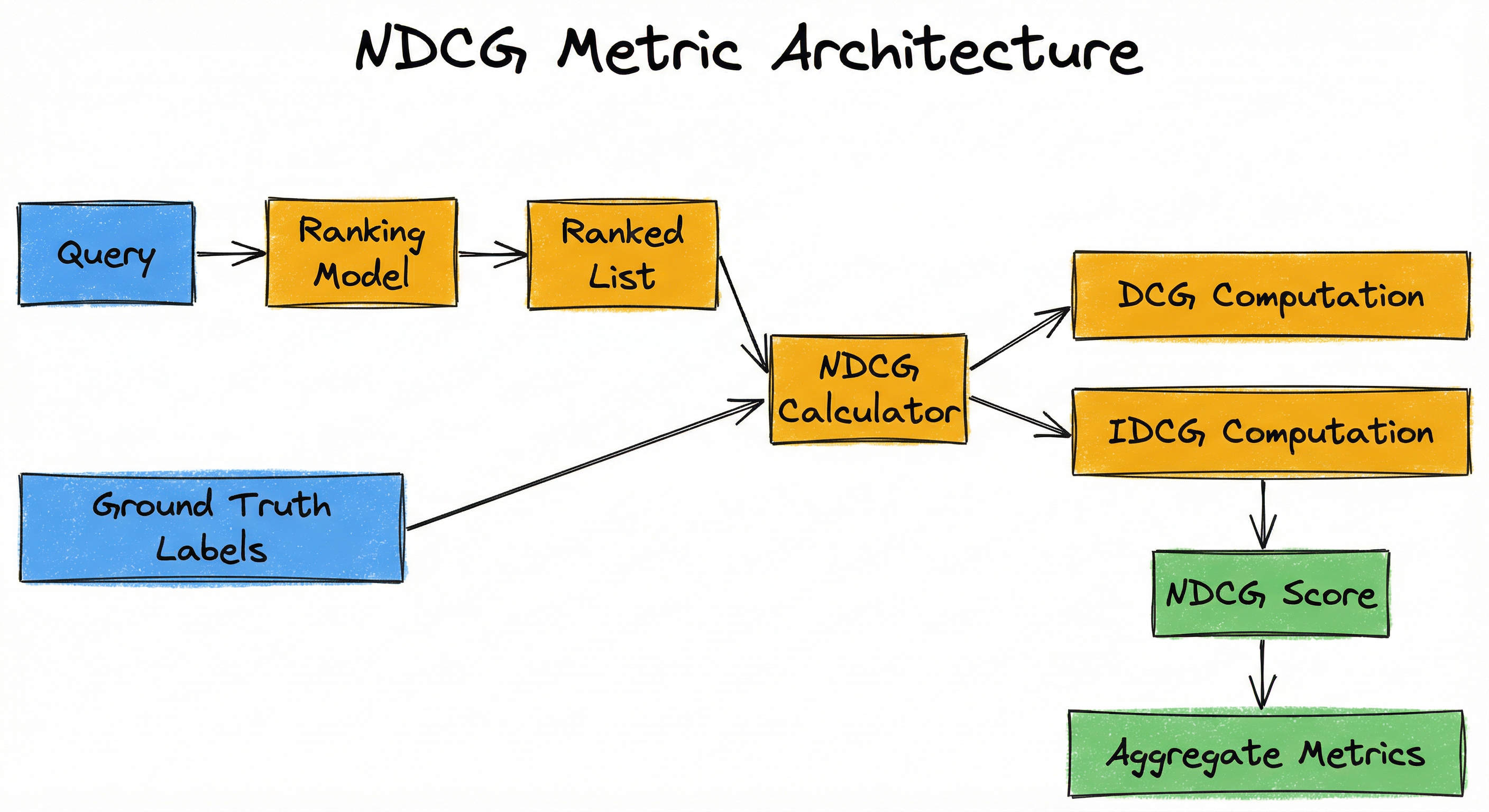
NDCG doesn't have a "system architecture" in the traditional sense -- it's a metric, not a deployable system. But there is a computational architecture for how it's calculated and integrated into ML pipelines. Let's map out the data flow from ranking model to NDCG score.
Key Components
Ranking Model
Produces a scored, ordered list of documents/items for a given query. Could be BM25, a learning-to-rank model, a neural ranker, or any ranking algorithm.
Ground Truth Labels
Human-annotated relevance judgments for query-document pairs, typically on a 0-4 graded scale. This is your gold standard for what "good" looks like.
DCG Calculator
Takes the ranked list and ground-truth labels, applies the DCG formula with position discounting. Outputs a single DCG value representing cumulative discounted gain.
IDCG Calculator
Sorts the same documents by descending relevance (creating the ideal ranking), computes DCG on this perfect order. This is the normalization denominator.
NDCG Score
Divides DCG by IDCG to produce the final normalized score between 0 and 1. This is the metric you track.
Aggregation Layer
Averages NDCG across multiple queries to get mean NDCG (the standard reporting metric). May also compute per-category NDCG for drill-down analysis.
Data Flow
Here's the data flow in a typical offline evaluation:
Input: A test set of queries with ground-truth relevance labels for candidate documents.
For each query :
- Ranking model produces a ranked list
- Retrieve ground-truth relevance scores for
- Compute using the formula
- Sort documents by descending relevance to get ideal order
- Compute using the ideal order
- Calculate
Output: Mean NDCG@K =
In online A/B testing, the flow is similar but fed by live traffic: user queries generate rankings, implicit feedback (clicks, dwell time) proxies for relevance labels, and NDCG is computed over cohorts.
A directed flow from 'Query' -> 'Ranking Model' -> 'Ranked List'. Separately, 'Ground Truth Labels' feed into an 'NDCG Calculator' that also receives the 'Ranked List', then flows through 'DCG Computation' -> 'IDCG Computation' -> 'NDCG Score' -> 'Aggregate Metrics'.
How to Implement
Three Approaches to Implementation
There are three common ways to compute NDCG in practice:
Option A: Use scikit-learn's ndcg_score -- easiest for Python users, supports both binary and graded relevance, handles the exponential gain formula by default. Great for prototyping and standard use cases.
Option B: Use LightGBM or XGBoost with ndcg evaluation metric -- essential when training learning-to-rank models. The GBDT libraries optimize directly for NDCG (or approximations like LambdaMART) during training.
Option C: Implement from scratch -- necessary when you need custom variations (different discount functions, alternative gain formulas, or integration with proprietary systems). Not hard if you understand the formula.
For production search/recommendation systems, you'll typically see Option B during training and Option A during offline evaluation. Let's walk through all three.
Cost Note: Computing NDCG itself is free (it's just math), but acquiring ground-truth labels is expensive. Budget INR 50-150 per query-document annotation if using crowdsourcing platforms like Amazon MTurk or Appen. For 1000 queries × 20 documents = 20,000 labels, expect to spend INR 10-30 lakh.
from sklearn.metrics import ndcg_score
import numpy as np

# Ground truth: rows = queries, cols = documents
# Each value is a relevance score (0-4 scale)
y_true = np.array([
    [3, 2, 3, 0, 1],  # Query 1: docs have rel [3,2,3,0,1]
    [4, 3, 2, 1, 0],  # Query 2: docs have rel [4,3,2,1,0]
])

# Model predictions: rows = queries, cols = documents
# Each value is a predicted score (higher = more relevant)
y_score = np.array([
    [0.9, 0.5, 0.8, 0.1, 0.3],  # Query 1: model scores
    [0.95, 0.85, 0.65, 0.45, 0.15],  # Query 2: model scores
])

# Compute NDCG@5 (default is exponential gain: 2^rel - 1)
ndcg_at_5 = ndcg_score(y_true, y_score, k=5)
print(f"NDCG@5: {ndcg_at_5:.4f}")
# Output: NDCG@5: 0.9623

# Compute NDCG@3 (top-3 only)
ndcg_at_3 = ndcg_score(y_true, y_score, k=3)
print(f"NDCG@3: {ndcg_at_3:.4f}")

# Per-query NDCG (useful for debugging)
for i, (true, score) in enumerate(zip(y_true, y_score)):
    ndcg = ndcg_score([true], [score], k=5)
    print(f"Query {i+1} NDCG@5: {ndcg:.4f}")
Scikit-learn's ndcg_score expects true relevance labels in y_true and model scores in y_score. It internally ranks documents by y_score (descending), maps those ranks to the relevance labels in y_true, then applies the DCG formula. The k parameter sets the cutoff -- NDCG@5 only considers the top 5 documents. By default, it uses the exponential gain formula (2^rel - 1).
import lightgbm as lgb
import numpy as np

# Features: shape (n_samples, n_features)
X = np.random.rand(1000, 20)

# Relevance labels: shape (n_samples,)
y = np.random.randint(0, 5, size=1000)

# Group sizes: number of documents per query
# Example: first 100 docs belong to query 1, next 150 to query 2, etc.
group = [100, 150, 200, 250, 300]

# Create dataset with group information
train_data = lgb.Dataset(X, label=y, group=group)

# LambdaRank parameters
params = {
    'objective': 'lambdarank',
    'metric': 'ndcg',
    'eval_at': [1, 3, 5, 10],  # Compute NDCG@1, @3, @5, @10
    'lambdarank_truncation_level': 10,
    'learning_rate': 0.05,
    'num_leaves': 31,
}

# Train the model
bst = lgb.train(
    params,
    train_data,
    num_boost_round=100,
    valid_sets=[train_data],
    callbacks=[lgb.log_evaluation(10)]
)

# The model directly optimizes NDCG during training
# Evaluation shows NDCG@1, NDCG@3, NDCG@5, NDCG@10
LightGBM's LambdaRank objective optimizes a differentiable approximation to NDCG called LambdaMART. The group parameter is crucial -- it tells LightGBM which documents belong to which query, since NDCG is a per-query metric. The eval_at parameter computes NDCG at multiple K values during training. This is the production approach for learning-to-rank models.
import numpy as np

def dcg_at_k(relevances, k):
    """Compute DCG@K for a single query."""
    relevances = np.asarray(relevances)[:k]
    if relevances.size == 0:
        return 0.0
    # DCG = sum of (2^rel - 1) / log2(position + 1)
    discounts = np.log2(np.arange(2, relevances.size + 2))
    gains = 2**relevances - 1
    return np.sum(gains / discounts)

def ndcg_at_k(true_relevances, predicted_scores, k):
    """Compute NDCG@K for a single query.

    Args:
        true_relevances: list of ground-truth relevance scores
        predicted_scores: list of model prediction scores
        k: cutoff position

    Returns:
        NDCG@K score between 0 and 1
    """
    # Sort by predicted scores (descending) and get relevances in that order
    sorted_indices = np.argsort(predicted_scores)[::-1]
    sorted_relevances = np.array(true_relevances)[sorted_indices]

    # Compute DCG for the predicted ranking
    dcg = dcg_at_k(sorted_relevances, k)

    # Compute IDCG for the ideal ranking (sorted by descending relevance)
    ideal_relevances = sorted(true_relevances, reverse=True)
    idcg = dcg_at_k(ideal_relevances, k)

    if idcg == 0:
        return 0.0

    return dcg / idcg

# Example usage
true_rel = [3, 2, 3, 0, 1, 2]
pred_scores = [0.9, 0.5, 0.8, 0.1, 0.3, 0.6]

ndcg = ndcg_at_k(true_rel, pred_scores, k=5)
print(f"NDCG@5: {ndcg:.4f}")
# Output: NDCG@5: 0.9570
This implementation follows the standard NDCG formula directly. The key steps are: (1) rank documents by predicted scores, (2) compute DCG using the actual relevance values in that ranked order, (3) compute IDCG by sorting relevances in descending order, (4) divide DCG by IDCG. The discount factor is log2(position + 1), and gain is 2^rel - 1. This gives you full control and transparency.
from redis import Redis
from redis.commands.search.query import Query
import numpy as np
from sklearn.metrics import ndcg_score

# Connect to Redis with RediSearch + vector similarity
client = Redis(host='localhost', port=6379, decode_responses=True)

# Example: evaluate NDCG@10 for semantic search
query_text = "best restaurants in Mumbai"
query_embedding = encode_query(query_text)  # Your encoder

# Search with vector similarity
q = Query("*=>[KNN 20 @embedding $vec AS score]")\
    .return_fields("id", "score")\
    .sort_by("score", asc=False)\
    .dialect(2)

results = client.ft("restaurants").search(
    q, query_params={"vec": query_embedding}
)

# Get ground truth relevance labels (from test set)
doc_ids = [doc.id for doc in results.docs]
true_relevances = get_labels(query_text, doc_ids)  # Your labeling

# Redis returns sorted by score, so predicted_scores are implicit
predicted_scores = [float(doc.score) for doc in results.docs]

# Compute NDCG@10
ndcg = ndcg_score([true_relevances], [predicted_scores], k=10)
print(f"NDCG@10 for query '{query_text}': {ndcg:.4f}")
This example shows how to evaluate NDCG for a vector similarity search system backed by Redis. The key insight: the ranking model is implicit (vector similarity), but NDCG evaluation is the same -- retrieve results, map to ground-truth labels, compute the metric. This pattern applies to any ranking system: BM25, neural rankers, collaborative filtering, etc.
# LightGBM ranking config (YAML equivalent)
objective: lambdarank
metric: ndcg
eval_at: [1, 3, 5, 10, 20]
lambdarank_truncation_level: 20
learning_rate: 0.05
num_leaves: 31
max_depth: -1
min_data_in_leaf: 20
feature_fraction: 0.8
bagging_fraction: 0.8
bagging_freq: 5
lambda_l1: 0.1
lambda_l2: 0.1
Common Implementation Mistakes
- ●
Using NDCG when you only care about the top-1 result -- in this case, MRR (Mean Reciprocal Rank) is more interpretable and aligns better with the objective. NDCG@1 reduces to a binary metric anyway.
- ●
Ignoring the K parameter and computing full-list NDCG when users never scroll past K=10 results. Always set K to match real user behavior. For mobile search, K=5 is often more realistic than K=20.
- ●
Mixing up the order of y_true and y_score in scikit-learn's ndcg_score. Remember: y_true is the ground truth relevance, y_score is what your model predicted. Swapping them gives nonsense results.
- ●
Comparing NDCG scores across datasets with different relevance scales. If dataset A uses 0-2 labels and dataset B uses 0-4, NDCG values aren't directly comparable due to the exponential gain formula. Always normalize labels first.
- ●
Forgetting that NDCG requires ground-truth labels for every ranked document. If you only have labels for a subset, you'll get partial NDCG (which is valid but requires careful interpretation). Missing labels for highly-ranked documents severely distort the metric.
- ●
Using online metrics (clicks, conversions) as a direct proxy for NDCG labels without calibration. Click position bias is real -- position 1 gets clicks even for mediocre results. De-bias clicks using inverse propensity scoring before treating them as relevance labels.
When Should You Use This?
Use When
Your application produces ranked lists where both relevance and position matter (search engines, recommendation feeds, document retrieval)
You have graded relevance labels (0-4 scale) rather than just binary relevant/not-relevant -- NDCG's strength is capturing gradations
You need a single metric that's comparable across queries of varying difficulty (different numbers of relevant docs)
Users exhibit position bias -- they scan from top to bottom and rarely scroll past K results
You're optimizing a learning-to-rank model and want the training objective to align with the evaluation metric (LambdaMART optimizes NDCG directly)
You need to compare multiple ranking algorithms on the same dataset -- NDCG provides a normalized, interpretable score
Avoid When
You only care about the top-1 result (use MRR or Success@1 instead -- simpler and more interpretable)
Relevance is strictly binary (relevant/not relevant) and you care about all relevant items equally, not position (use MAP or recall@K instead)
You don't have ground-truth relevance labels and can't afford to collect them (NDCG requires labels; consider implicit metrics like click-through rate)
Your ranking task has exactly one correct answer per query (use reciprocal rank instead -- NDCG is overkill)
You need a metric that penalizes bad recommendations more heavily -- NDCG doesn't penalize irrelevant items as strongly as some alternatives
Key Tradeoffs
The Core Tradeoff: Complexity vs. Informativeness
NDCG is more complex than simpler metrics like precision@K or recall@K, but it captures information they can't: the interaction between relevance and position. The question is whether that complexity pays for itself.
When the complexity is worth it: If you're building Google Search or Amazon product ranking, NDCG is non-negotiable. The difference between a good ranking and a great ranking directly impacts revenue and user satisfaction. The metric needs to distinguish those gradations.
When simpler metrics suffice: If you're building a yes/no classifier with a short ranked list (like "top 3 related articles"), precision@3 might be enough. Don't over-engineer the metric if the task is simple.
Graded Relevance vs. Binary Labels
NDCG's advantage is graded relevance (0-4 scale), but that comes at a cost: annotation difficulty. Getting consistent 5-level judgments from crowdworkers is hard and expensive. Binary labels (relevant/not) are faster and cheaper.
Rule of thumb: use graded labels when relevance differences are meaningful and observable. For product search, the difference between "perfect match" and "close match" matters. For duplicate detection, it's usually binary (duplicate or not).
NDCG@K: Picking the Right K
Smaller K (like NDCG@5) focuses on top results and is more sensitive to swaps among top positions. Larger K (like NDCG@100) captures overall ranking quality but is less sensitive to top-position changes.
For user-facing search, choose K based on viewport size and user behavior:
- Mobile search: K=5 (users rarely scroll)
- Desktop search: K=10 to 20
- Recommendation carousels: K = number of visible items (usually 6-12)
- Document retrieval for RAG: K = number of docs fed to LLM (often 3-10)
Key Insight: There's no universal K. Match it to your UI and user behavior. Track multiple K values (NDCG@1, @3, @5, @10) to understand the full quality curve.
Alternatives & Comparisons
MAP is the average of precision values computed at each relevant document position. It's position-aware (like NDCG) but assumes binary relevance. Use MAP when you only have binary labels and care about all relevant items, not just top-K. NDCG is more flexible (supports graded relevance) and more commonly used in modern ranking systems. MAP is still popular in academic IR benchmarks.
MRR measures the average inverse rank of the first relevant result (1/rank). It's perfect for tasks with one correct answer ("Where is the capital of France?") but ignores all results after the first relevant one. Use MRR for navigational search or QA systems; use NDCG for exploratory search where multiple results are useful. MRR is simpler and more interpretable but captures less information.
Precision@K is the fraction of top-K results that are relevant. It's position-unaware: swapping items within the top-K doesn't change the score. Use Precision@K when you only care about the count of relevant items, not their order. NDCG is strictly more informative (it subsumes position information) but harder to interpret. For simple cases, Precision@K is often enough.
Recall@K measures what fraction of all relevant documents appear in the top-K. It's position-unaware and focuses on coverage rather than ranking quality. Use Recall@K when retrieving a candidate set for re-ranking (you want to maximize relevant items, order doesn't matter yet). NDCG is better for evaluating the final ranked list shown to users.
Pros, Cons & Tradeoffs
Advantages
Position-aware: heavily rewards placing relevant items at the top, aligning with how users actually consume ranked lists. A result at position 1 is worth exponentially more than at position 10.
Graded relevance: supports multi-level relevance scales (0-4), capturing nuances that binary metrics miss. A perfect match is worth more than a good match, as it should be.
Normalized across queries: NDCG scores from 0 to 1 are comparable regardless of how many relevant documents exist. You can meaningfully average NDCG across queries with different difficulty.
Widely adopted in industry: Google, Amazon, Netflix, and most major tech companies use NDCG as a primary ranking metric. This means extensive tooling support (scikit-learn, LightGBM, TensorFlow Ranking).
Aligns with learning-to-rank objectives: LambdaMART and other gradient-boosted rankers can optimize NDCG directly, so your training objective matches your evaluation metric.
Handles tied relevance scores gracefully: documents with the same relevance contribute proportionally to DCG based on their position.
Supports multiple K values: you can compute NDCG@5, @10, @20 simultaneously to understand ranking quality at different depths.
Disadvantages
Requires ground-truth labels: you need human-annotated relevance judgments for every query-document pair you want to evaluate. This is expensive (INR 50-150 per label) and time-consuming.
Doesn't penalize missing documents: if your ranker returns fewer than K documents, NDCG doesn't penalize that. A query returning 5 results can score the same as one returning 10, even if more relevant docs exist.
Doesn't penalize bad recommendations as heavily: adding an irrelevant document at position 10 barely affects NDCG, even though it might harm user experience. The log discount makes low positions almost free.
Low interpretability: what does NDCG=0.76 mean in absolute terms? It's relative to the ideal ranking, but not as intuitive as "3 out of 5 results were relevant" (Precision@5).
Sensitive to relevance scale: if annotators use only the top 2 levels of a 0-4 scale, NDCG behaves differently than if they use all levels. You need annotation guidelines and quality control.
Assumes logarithmic position discount: the log2 formula is empirically validated but not universal. Some user populations might exhibit different attention curves (power-law, linear).
Computationally heavier than simpler metrics: DCG requires sorting and iterating over top-K results for each query. For millions of queries, this adds up (though it's still fast in practice).
Failure Modes & Debugging
Incomplete relevance labels
Cause
Ground-truth labels exist for only a subset of retrieved documents (e.g., labels for top-10, but the model returns top-20). Unlabeled documents are typically treated as irrelevant (rel=0), distorting NDCG.
Symptoms
NDCG scores drop unexpectedly when the model retrieves documents outside the labeled set. A model that returns 20 documents (10 labeled, 10 unlabeled) scores lower than one returning only the labeled 10, even if the extra 10 are relevant.
Mitigation
Use pooling strategies during annotation: collect top-K results from multiple baseline models and label the union. Alternatively, compute NDCG only on the labeled subset and report it as partial NDCG with a caveat. For production systems, continuously collect labels for new documents as they appear.
Position bias in implicit labels
Cause
Using click-through data as a proxy for relevance without correcting for position bias. Users click on position 1 at much higher rates than position 5, even when both are equally relevant.
Symptoms
Models optimized for click-based NDCG over-rank documents at top positions because the training signal is biased. The model learns to exploit position bias rather than true relevance.
Mitigation
Apply inverse propensity scoring (IPS) to de-bias clicks: weight each click by 1/P(click | position). Use randomized experiments to estimate position-dependent click probabilities. Alternatively, use explicit human judgments for evaluation, even if training uses implicit signals.
Mismatched K between training and evaluation
Cause
Training a model to optimize NDCG@100 but evaluating on NDCG@10 (or vice versa). The model learns to optimize for the wrong depth.
Symptoms
Model performs well on NDCG@100 but poorly on NDCG@10. The ranker spreads relevant documents across positions 1-100 instead of concentrating them in the top 10.
Mitigation
Always match the K used during training and evaluation. If multiple K values matter (e.g., NDCG@5 and @10), train the model with the smallest K you care about -- optimization for NDCG@5 usually improves NDCG@10 as a side effect.
Annotation quality drift
Cause
Relevance labels collected at different times or by different annotator pools exhibit inconsistent standards. What counts as "highly relevant" shifts over time.
Symptoms
NDCG scores fluctuate when re-evaluating the same model on new annotation batches. Models trained on old labels underperform on new labels, even though the data distribution hasn't changed.
Mitigation
Establish and enforce annotation guidelines with concrete examples ("4 = perfect answer to the query, 3 = good but not perfect, etc."). Include gold-standard queries with known labels in every annotation batch to monitor annotator agreement. Retrain annotators periodically and measure inter-annotator agreement (Krippendorff's alpha or Fleiss' kappa).
Zero IDCG edge case
Cause
All documents for a query have relevance 0 (no relevant results exist). IDCG = 0, so NDCG = 0/0 is undefined.
Symptoms
Code crashes with division-by-zero error, or NDCG is returned as NaN or 0, both of which skew aggregate metrics.
Mitigation
Handle the zero-IDCG case explicitly: return NDCG = 0 (convention) or exclude the query from mean NDCG calculation (depends on your goal). Scikit-learn returns 0 by default. Document this behavior in your evaluation code.
Overfitting to NDCG on small test sets
Cause
Tuning hyperparameters or model architecture to maximize NDCG on a small validation set (e.g., 50 queries). The model overfits to the specific queries in the set.
Symptoms
NDCG improves on the validation set but degrades on a held-out test set or in A/B testing. The model memorizes quirks of the validation queries rather than learning generalizable patterns.
Mitigation
Use larger validation sets (minimum 500-1000 queries for stable NDCG estimates). Use cross-validation if labels are limited. Reserve a separate test set for final evaluation and never tune on it. Track the variance of NDCG (compute confidence intervals via bootstrapping) to avoid overfitting to noise.
Placement in an ML System
Where Does NDCG Sit in the Pipeline?
NDCG is a metric, not a component of the inference pipeline. It lives in the evaluation and monitoring layer, not the serving path. Here's the conceptual architecture:
Training time: A learning-to-rank model (LightGBM LambdaRank, neural ranker) optimizes NDCG (or a differentiable proxy) as its objective function. NDCG guides what the model learns.
Offline evaluation: After training, you evaluate the model on a held-out test set by computing mean NDCG@K across all test queries. This is your primary quality metric.
A/B testing: When deploying a new ranking model, you serve it to a small percentage of users and compute NDCG on their queries (using post-hoc labels from clicks or explicit feedback). Compare to the baseline model's NDCG.
Monitoring: In production, continuously track NDCG on a fixed set of "canary queries" with known labels. If NDCG drops below a threshold, trigger an alert -- the model may have degraded.
NDCG never touches the user-facing serving path. It's strictly a measurement tool for offline and online evaluation.
Key Insight: NDCG is to ranking what accuracy is to classification -- the primary offline metric for model quality. But unlike accuracy, NDCG can also be estimated online using implicit feedback, making it a bridge between offline evaluation and live A/B testing.
Pipeline Stage
Evaluation / Metrics
Upstream
- Ranking Model
- Search Engine
- Recommendation System
- Document Retriever
- Ground Truth Annotation Pipeline
Downstream
- Model Selection
- Hyperparameter Tuning
- A/B Testing Framework
- Monitoring Dashboard
Scaling Bottlenecks
NDCG computation itself is fast -- per query (dominated by sorting documents by predicted scores). For 1 million queries with K=20, this takes a few seconds on a single CPU core. This is not a bottleneck.
The real bottleneck is label acquisition. Collecting ground-truth labels for 1000 queries × 20 documents = 20,000 labels at INR 100 per label costs INR 20 lakh and requires weeks of annotation time. Annotation quality control (verifying inter-annotator agreement, filtering low-quality workers) adds another 20-30% overhead.
For production systems with millions of queries, you can't label everything. Strategies:
- Sample queries strategically: Focus on high-traffic queries (power law: top 1% of queries account for 50% of traffic) and edge cases (tail queries, new query types).
- Use active learning: Train an initial model, identify queries where the model is most uncertain, label those preferentially.
- Leverage implicit feedback: Use clicks, dwell time, and conversions as noisy proxies for relevance. De-bias with inverse propensity scoring. This scales to billions of queries.
- Continuous annotation: Budget a fixed annotation spend per month (e.g., INR 2 lakh/month) and continuously label new queries as the system evolves.
If you're running NDCG evaluation in a CI/CD pipeline or A/B testing framework, optimize by:
- Pre-sorting documents by predicted scores once, reusing for all K values (NDCG@5, @10, @20 from a single sort)
- Vectorizing DCG computation (NumPy/PyTorch over loops)
- Parallelizing across queries (embarrassingly parallel -- each query is independent)
Production Case Studies
Google uses NDCG internally to evaluate search quality across billions of queries. In their 2013 paper "Measuring Search Engine Quality using Random Walks on the Click Graph," they discuss how NDCG correlates with user satisfaction metrics. Google's human raters provide graded relevance judgments (Perfect, Excellent, Good, Fair, Bad) for query-document pairs, which map directly to NDCG's 0-4 scale. The company runs thousands of ranking experiments annually, using NDCG as a primary metric to compare variants.
NDCG enables rigorous, repeatable evaluation of ranking changes at scale. Improvements of 0.01-0.02 in mean NDCG translate to measurable gains in user engagement and satisfaction, guiding search quality roadmaps.
Airbnb uses NDCG to evaluate its search ranking for Experiences (activities and tours). They collect ground-truth labels by analyzing booking behavior: experiences that users book are labeled as highly relevant (rel=4), those clicked but not booked as moderately relevant (rel=2), and those not interacted with as irrelevant (rel=0). They train a gradient-boosted decision tree model (LightGBM) to optimize NDCG@10, since users rarely scroll past the first 10 results on mobile.
Optimizing for NDCG@10 (rather than simpler metrics like click-through rate) improved booking conversion rate by 13% and increased overall bookings of Experiences. NDCG's position awareness ensured that high-conversion experiences appeared at the top, maximizing user satisfaction and revenue.
Spotify uses Normalized Discounted Cumulative Gain (NDCG@k) as a key metric for evaluating recommendation models that personalize content on the Home screen. The metric helps correlate offline model performance with online engagement metrics.
Through A/B testing, Spotify correlated NDCG scores with online metrics like the amount of listens coming from recommended sections. NDCG serves as a common metric across many of Spotify's recommendation systems for ranking quality evaluation.
Flipkart uses NDCG to evaluate product search relevance. Human annotators (based in India) label query-product pairs on a 0-4 scale: 4 = perfect match (e.g., query "iPhone 15 Pro" returns the exact product), 3 = good match (same brand/model but different variant), 2 = somewhat relevant (same category), 1 = marginally relevant, 0 = irrelevant. They compute NDCG@20 for desktop and NDCG@10 for mobile (reflecting viewport sizes). Ranking models are trained using XGBoost with NDCG as the objective.
A 2% improvement in NDCG@10 (from 0.78 to 0.80) correlated with a 5% increase in search-to-cart conversion rate in A/B tests. The graded relevance scale helped distinguish between "close enough" and "perfect match," which matters in e-commerce where users have specific intent.
Netflix uses NDCG to evaluate its recommendation carousels ("Top Picks for You," "Trending Now," etc.). Relevance is inferred from user behavior: titles the user watches to completion are labeled as highly relevant, those partially watched as moderately relevant, and those not clicked as irrelevant. They compute NDCG@K where K is the number of visible items in the carousel (typically 6-12 on different devices). Position matters enormously: items on the left of the carousel get 10x more attention than items on the right.
Optimizing for NDCG (rather than just click-through rate) increased hours watched per user by 4% in A/B tests. NDCG's position discount aligned with the reality of carousel UX -- users scan left to right and rarely scroll -- making it a better proxy for user satisfaction than position-unaware metrics.
Tooling & Ecosystem
Python library providing ndcg_score function for computing NDCG@K. Supports both binary and graded relevance, exponential gain formula (2^rel - 1) by default. Best for offline evaluation and prototyping.
Gradient boosting framework with built-in LambdaRank objective that optimizes NDCG directly. Supports eval_at parameter to compute NDCG@1, @3, @5, @10 during training. Industry standard for learning-to-rank.
Gradient boosting library with rank:ndcg objective based on LambdaMART. Similar to LightGBM but with different implementation. Supports multi-GPU training for large-scale ranking.
TensorFlow library for learning-to-rank with neural networks. Provides differentiable approximations to NDCG (ApproxNDCG, NeuralNDCG) for gradient-based optimization. Best for deep learning ranking models.
Java library implementing LambdaMART, AdaRank, and other learning-to-rank algorithms with NDCG evaluation. Popular in academic IR research. Slower than LightGBM but more algorithms.
Python toolkit for reproducible IR research built on Apache Lucene. Includes utilities for computing NDCG and other ranking metrics on standard IR benchmarks (MS MARCO, TREC).
Python library providing a unified interface to compute 20+ IR metrics including NDCG, MAP, MRR, and more. Useful for benchmarking across multiple metrics simultaneously.
Research & References
Järvelin, K. & Kekäläinen, J. (2002)ACM Transactions on Information Systems (TOIS), Vol. 20, No. 4
The original NDCG paper. Introduced discounted cumulative gain (DCG) and normalized DCG (NDCG) as position-aware, graded-relevance metrics for IR evaluation. Showed that NDCG correlates better with user satisfaction than binary metrics. This is the foundational reference -- cite this if you use NDCG.
Wang, Y., Wang, L. & Li, Y. (2013)COLT 2013 (Conference on Learning Theory)
Provides theoretical analysis of NDCG's properties: decomposition into position-dependent sub-metrics, axiomatic justification for the log discount, and analysis of NDCG's consistency as a ranking measure. Shows NDCG satisfies desirable properties like permutation invariance and monotonicity.
Xu, J. & Li, H. (2007)NeurIPS 2007
Introduced AdaRank, an algorithm that directly optimizes NDCG during training (rather than a surrogate loss). Showed that optimizing NDCG directly outperforms pointwise and pairwise methods on LETOR benchmark datasets. Foundational work for listwise learning-to-rank.
Burges, C. J. (2010)Microsoft Research Technical Report MSR-TR-2010-82
Describes the evolution of gradient-based ranking models: RankNet (pairwise), LambdaRank (NDCG-aware gradients), and LambdaMART (LambdaRank + MART gradient boosting). LambdaMART became the industry standard for NDCG optimization and is implemented in LightGBM and XGBoost.
Pobrotyn, P., Bartczak, T., Synowiec, M. et al. (2021)AAAI 2021
Introduced a fully differentiable approximation to NDCG using NeuralSort, enabling end-to-end gradient-based optimization of NDCG in neural ranking models. Showed that direct NDCG optimization outperforms cross-entropy and pairwise losses on several benchmarks.
Yang, Y., Wang, Y. & Zhang, Y. (2024)arXiv preprint
Recent work (2024) applying differentiable NDCG to LLM preference alignment and RLHF. Shows that optimizing NDCG over ranked preferences improves LLM output quality compared to Bradley-Terry pairwise models. Extends NDCG to the LLM era.
Zhan, Y., Wan, M. & Wang, J. (2023)arXiv preprint
Analyzes NDCG's suitability for off-policy evaluation in recommender systems. Shows that NDCG can be biased when using logged data (due to position bias and incomplete feedback) and proposes inverse propensity scoring corrections.
Zuo, Y., Zeng, J., Gong, M. & Jiao, L. (2019)Industry blog / technical exposition
Clear, detailed explanation of how LambdaMART combines gradient boosting (MART) with NDCG-aware lambda gradients from LambdaRank. Includes implementation details, hyperparameter tuning tips, and comparisons to other learning-to-rank methods. Excellent practical resource.
Interview & Evaluation Perspective
Common Interview Questions
- ●
Explain NDCG in simple terms. Why is it better than precision or recall?
- ●
How would you collect ground-truth labels for NDCG evaluation?
- ●
What's the difference between DCG and IDCG? Why do we normalize?
- ●
When would you use NDCG vs. MRR vs. MAP?
- ●
How does LambdaMART optimize NDCG during training?
- ●
Your NDCG@10 is 0.75. Is that good or bad? How would you improve it?
- ●
How do you handle position bias when using click data to compute NDCG?
Key Points to Mention
- ●
NDCG is position-aware (discounts by log2(position+1)) and supports graded relevance (0-4 scale), making it ideal for ranking evaluation where both relevance and order matter.
- ●
The normalization step (dividing by IDCG) makes NDCG comparable across queries with different numbers of relevant documents -- critical for aggregating across a test set.
- ●
NDCG@K (e.g., @5, @10) lets you focus on top-K results. Choose K based on user behavior: mobile users rarely scroll past 5 results, desktop users might see 10-20.
- ●
Ground-truth labels are expensive -- budget INR 50-150 per annotation. For production systems, use pooling (label the union of top-K from multiple models) to maximize coverage.
- ●
LambdaMART (in LightGBM/XGBoost) optimizes a differentiable approximation to NDCG by computing lambda gradients -- gradients based on how swapping document pairs affects NDCG.
- ●
NDCG doesn't penalize missing documents or heavily penalize low-position irrelevant items -- be aware of these limitations when choosing it as your metric.
Pitfalls to Avoid
- ●
Confusing NDCG with accuracy or F1 -- NDCG is for ranking (ordered lists), not classification (binary/multiclass predictions). Don't say "we can use NDCG to evaluate a classifier."
- ●
Claiming NDCG works without ground-truth labels -- it requires human judgments or high-quality implicit feedback. You can't compute NDCG from model scores alone.
- ●
Ignoring position bias when using clicks as labels -- raw click data is biased toward top positions. Always mention de-biasing (inverse propensity scoring) if you propose using clicks.
- ●
Treating NDCG as a black box without explaining the DCG formula or normalization -- in a senior interview, you should be able to walk through the math.
- ●
Not discussing the choice of K -- saying "we'll use NDCG" without specifying K shows you haven't thought about the application. Always justify your K choice based on UI/UX.
Senior-Level Expectation
A senior candidate should discuss the full evaluation pipeline: annotation strategy (how to collect labels cost-effectively), choice of K and relevance scale, handling edge cases (zero IDCG, incomplete labels), position bias in implicit feedback, alignment between training objective (LambdaMART) and evaluation metric (NDCG), A/B testing with online NDCG, and tradeoffs vs. alternative metrics (MAP, MRR). They should also justify why NDCG is appropriate for the specific ranking task at hand -- not all ranking problems need NDCG. For example, if the task has a single correct answer, MRR is simpler and more interpretable. Senior engineers reason about metric choice based on user behavior, data availability, and business objectives, not just "industry best practices."
Summary
Let's recap the key points:
-
NDCG (Normalized Discounted Cumulative Gain) is a ranking evaluation metric that measures how well a ranked list matches an ideal ordering by accounting for both graded relevance (0-4 scale) and position (with logarithmic discounting).
-
The formula is where DCG sums discounted relevance scores and IDCG is the DCG of the perfect ranking. Scores range from 0 to 1.
-
Position matters enormously: NDCG discounts by , meaning position 1 is worth ~3x more than position 10. This aligns with user behavior -- people scan from top to bottom.
-
Normalization enables comparison: Dividing by IDCG makes NDCG comparable across queries with different numbers of relevant documents. You can meaningfully average NDCG across a test set.
-
NDCG@K is task-specific: Choose K based on user behavior. Mobile search: K=5. Desktop search: K=10-20. Recommendation carousels: K = number of visible items. Don't use a generic K.
-
Label acquisition is the bottleneck: Computing NDCG is fast, but collecting ground-truth labels costs INR 50-150 per annotation. Use pooling strategies and implicit feedback to scale.
-
LambdaMART (LightGBM/XGBoost) optimizes NDCG directly using lambda gradients, making it the industry standard for learning-to-rank. Training objective aligns with evaluation metric.
-
Tradeoffs: NDCG is more informative than precision/recall (captures position and graded relevance) but less interpretable ("0.76" is harder to explain than "3 out of 5 relevant"). It requires labels and doesn't penalize missing documents.
NDCG is the gold standard for ranking evaluation when both relevance and position matter. It's the bridge between offline evaluation (human labels) and online metrics (user engagement). If you're building search, recommendations, or any system that produces ordered lists, NDCG is likely the metric you should optimize for.