Precision@K in Machine Learning
You've built a search engine, a recommendation feed, or a RAG pipeline. Users type a query, your system returns a ranked list of results. The fundamental question is: how many of those results are actually relevant?
That's exactly what Precision@K answers. It counts how many of the top K results your system returned are relevant, and divides by K. If you retrieve 10 documents and 7 are relevant, your P@10 is 0.7. Simple, interpretable, actionable.
Precision@K is arguably the most intuitive ranking metric in information retrieval. Unlike NDCG, which requires graded relevance scores and logarithmic discount factors, P@K works with binary labels: each result is either relevant or not. Unlike MAP, which averages precision across all recall levels, P@K gives you a single number that directly corresponds to user experience -- "out of the K items I showed the user, what fraction were useful?"
This metric has been a cornerstone of IR evaluation since the early TREC experiments in the 1990s, and it remains widely used today in production search engines, recommendation systems, and increasingly in RAG pipeline evaluation. From Google's search quality assessments to Flipkart's product ranking to evaluating whether your vector database retrieves the right context chunks for an LLM -- P@K is the metric you reach for when you want a quick, honest answer about retrieval quality.
In this guide, we'll cover the P@K formula in depth, explore when it's the right metric (and when it's not), walk through production implementations, and discuss the critical relationship between P@K and its sibling metrics: Recall@K, MAP, NDCG, and MRR.
Concept Snapshot
- What It Is
- A ranking evaluation metric that measures the fraction of retrieved items in the top K positions that are relevant, using binary relevance judgments (relevant or not relevant).
- Category
- Evaluation
- Complexity
- Beginner
- Inputs / Outputs
- Inputs: a ranked list of K retrieved items and binary relevance labels (relevant/not-relevant) for each item. Output: a single score between 0 and 1, where 1 means all top-K items are relevant.
- System Placement
- Used in offline evaluation of search engines, recommendation systems, retrieval components of RAG pipelines, and as an online metric in A/B testing for ranking quality.
- Also Known As
- P@K, Precision at K, Precision at top K, Precision at cutoff K, P@n
- Typical Users
- ML engineers, Search engineers, Recommendation system developers, RAG pipeline engineers, IR researchers, Data scientists
- Prerequisites
- Binary relevance concept, Ranked list basics, Precision and recall fundamentals, Information retrieval basics
- Key Terms
- binary relevancetop-K cutoffprecisionretrieval qualityranking evaluationrelevant itemsset-based metricmicro-averagingmacro-averaging
Why This Concept Exists
The Fundamental Problem: "Are My Results Any Good?"
Imagine you're running a product search on an e-commerce platform. A user searches for "wireless earbuds under 2000," and your system returns 10 results. How do you measure whether those results were good? You could measure recall -- but recall alone doesn't tell you about noise. If 8 out of 10 results are irrelevant, the user experience is terrible regardless of recall.
Precision@K solves this directly. It asks: "of the K items you showed me, how many were relevant?" If P@10 = 0.7, that means 7 out of 10 results were relevant. Simple, direct, actionable.
The TREC Legacy
Precision@K has deep roots in the TREC (Text REtrieval Conference) evaluations, organized by NIST starting in 1992. TREC established the standard methodology for evaluating IR systems: create a test collection with relevance judgments, run each system, and compare using metrics.
In the early TREC experiments, the primary metrics were precision at various cutoff depths: P@5, P@10, P@20. These cutoffs mapped to user behavior -- P@10 corresponds to the first page of search results. Ellen Voorhees and Chris Buckley's work at NIST showed that P@K was stable, interpretable, and correlated with user satisfaction.
From TREC to Production Systems
P@K transitioned from academic benchmarks to production systems because it maps directly to business outcomes:
- E-commerce search: P@10 directly impacts conversion rate
- Recommendation feeds: P@5 tells you how many recommendations are useful
- RAG pipelines: P@3 tells you how many context chunks passed to the LLM are relevant
- Content moderation: P@K tells you the fraction of flagged items that actually violate policies
Key Insight: P@K exists because it directly answers the question end-users implicitly ask: "Is this result page useful?" Its simplicity -- binary relevance, single cutoff, no position weighting -- is a feature, not a limitation.
Core Intuition & Mental Model
The Restaurant Analogy
Imagine you ask a friend to recommend 5 restaurants in Bangalore for dinner tonight. They suggest:
- A highly-rated biryani place (you love biryani) -- Relevant
- A new Italian restaurant with great reviews -- Relevant
- A bar that closed last month -- Not relevant
- A South Indian breakfast place (you want dinner) -- Not relevant
- A trending Korean BBQ spot -- Relevant
Your friend's Precision@5 = 3/5 = 0.6. Three out of five suggestions were useful. That's a decent score, but not great -- you had to mentally filter out 2 bad suggestions.
Now imagine a second friend gives you 5 recommendations and all 5 are excellent dinner options: P@5 = 1.0. That's the friend you trust more for restaurant advice.
That's P@K in a nutshell: out of K things you recommended, what fraction were actually relevant?
Why "At K" Matters
The "@K" part is crucial. Consider two search engines:
- Engine A: Returns 100 results. 50 are relevant. Precision = 0.5. But the first 10 results are all relevant (P@10 = 1.0).
- Engine B: Returns 100 results. 50 are relevant. Precision = 0.5. But the relevant results are scattered randomly (P@10 = 0.5).
Overall precision is identical, but Engine A is clearly superior for users who only look at the first page. P@10 captures this distinction -- it evaluates what users actually see.
The choice of K should match your UI and user behavior:
- Mobile search results page: K = 5 (users see ~5 results without scrolling)
- Desktop search results page: K = 10 (standard Google SERP)
- Recommendation carousel: K = number of visible items (often 6-8)
- RAG context window: K = number of chunks retrieved (often 3-5)
The Position Blindness Property
Here's the critical thing to understand about P@K: it doesn't care about order within the top K. These two result lists have the same P@5:
- List A: [Relevant, Relevant, Relevant, Irrelevant, Irrelevant] -- P@5 = 0.6
- List B: [Irrelevant, Irrelevant, Relevant, Relevant, Relevant] -- P@5 = 0.6
But List A is obviously better -- the relevant results are at the top, where users look first. P@K treats them as equally good. This is P@K's biggest limitation and the reason metrics like MAP and NDCG exist (they are position-aware).
Mental Model: Think of P@K as checking a box: "out of the K items in this box, how many are good?" It doesn't care how the items are arranged inside the box. If arrangement matters to you (it usually does in search), you need a position-aware metric like NDCG or MAP on top of P@K.
Technical Foundations
The Formula
For a query with a ranked list of retrieved items , Precision@K is defined as:
Equivalently, using an indicator function where 1 means relevant:
Properties
- Range:
- P@K = 1 when all top-K items are relevant
- P@K = 0 when no top-K items are relevant
- Position-invariant: The score is the same regardless of the ordering of relevant/irrelevant items within the top K
- K-dependent: Different K values yield different scores for the same ranked list
Worked Example
Suppose we retrieve 10 documents with the following relevance labels (1 = relevant, 0 = not relevant):
| Position | 1 | 2 | 3 | 4 | 5 | 6 | 7 | 8 | 9 | 10 |
|---|---|---|---|---|---|---|---|---|---|---|
| Relevant | 1 | 1 | 0 | 1 | 0 | 1 | 0 | 0 | 1 | 0 |
Precision at various cutoffs:
Notice how P@K generally decreases as K increases (unless you keep finding relevant documents). This makes intuitive sense: the further down you go, the more likely you are to encounter irrelevant items.
Relationship to Standard Precision
Standard precision in classification is:
P@K is exactly this, applied to the top-K cutoff:
- True Positives (TP): Relevant items in the top K
- False Positives (FP): Irrelevant items in the top K
- TP + FP = K (by construction, since we always return exactly K items)
So .
The Upper Bound Problem
A subtle but important issue: if there are only relevant documents in the entire corpus and , then even a perfect system cannot achieve P@K = 1. The maximum achievable precision is:
For example, if only 3 documents are relevant and K = 10, the best possible P@10 = 3/10 = 0.3. This is sometimes called the saturation problem and is why comparing P@K across queries with different numbers of relevant documents can be misleading.
Micro-Averaging vs. Macro-Averaging
When aggregating P@K across multiple queries:
Macro-averaged P@K (most common): Average P@K across all queries equally.
This gives equal weight to every query, regardless of how many relevant documents it has.
Micro-averaged P@K: Pool all top-K results across queries and compute a single precision.
This gives more weight to queries with more relevant documents. Macro-averaging is standard in most IR benchmarks (TREC, MS MARCO).
Implementation Note: Always report which averaging scheme you use. Macro-averaging is the default in academic papers and most libraries. Micro-averaging may be preferred in production when high-traffic queries are more important (since they naturally contribute more to the micro-average).
Internal Architecture
Precision@K is a metric computation, not a deployable service. But it has a well-defined computational architecture when integrated into an ML evaluation pipeline. Here's how P@K fits into a typical search or recommendation evaluation workflow.
The key architectural decision is where the relevance labels come from. In offline evaluation, they come from human annotations or gold-standard test sets. In online evaluation (A/B testing), they come from implicit feedback signals (clicks, purchases, dwell time) that proxy for relevance.
Key Components
Query Set
A collection of test queries with known relevance judgments. For offline evaluation, this comes from TREC-style test collections or in-house annotation projects. For online evaluation, queries are sampled from live traffic.
Retrieval System
The system under evaluation: a search engine, recommendation algorithm, vector similarity search, or RAG retriever. It takes a query and produces a ranked list of results.
Top-K Truncation
Truncates the ranked list to the first K positions. Only these K items are evaluated. Items beyond position K are ignored entirely, regardless of their relevance.
Relevance Labels
Binary labels (relevant=1, not-relevant=0) for each query-document pair. These are the ground truth against which the retrieval system is evaluated. Sources include human annotators, LLM-based labeling, or implicit feedback signals.
P@K Calculator
For each query, counts the number of relevant items in the top K and divides by K. Produces a per-query P@K score.
Aggregation Layer
Computes mean P@K (macro-averaged) across all queries. May also compute P@K per category, per query difficulty level, or per user segment for drill-down analysis.
Data Flow
The data flow for P@K evaluation follows these steps:
Step 1: Query Execution -- For each query in the test set , the retrieval system produces a ranked list .
Step 2: Top-K Truncation -- The ranked list is truncated to the first K positions: .
Step 3: Relevance Lookup -- For each document in , look up its binary relevance label from the ground-truth set.
Step 4: Per-Query P@K -- Compute .
Step 5: Aggregation -- Compute mean P@K: .
Step 6: Reporting -- Report mean P@K along with standard deviation, confidence intervals, and per-category breakdowns.
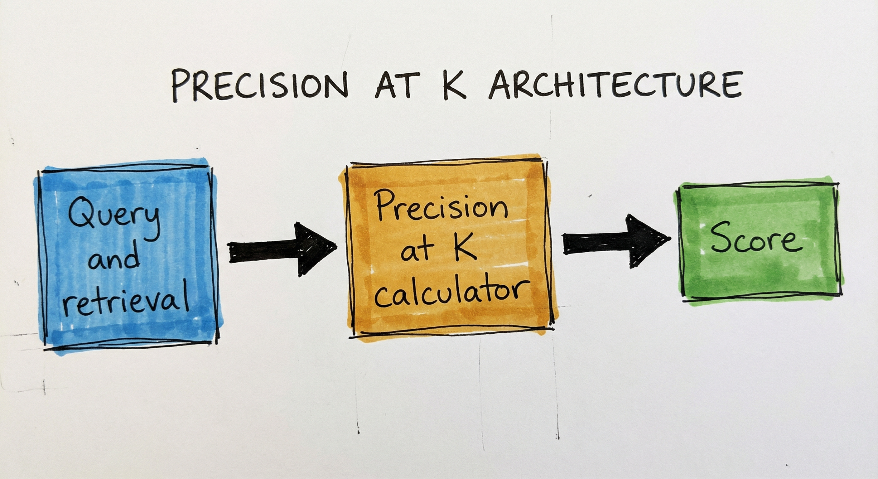
A directed flow diagram showing: 'Query Set' feeds into 'Retrieval System', which produces 'Top-K Results'. Separately, 'Relevance Labels' feed into a 'P@K Calculator' along with the Top-K Results. The calculator outputs 'Per-Query P@K' scores, which flow to 'Aggregation', then to 'Mean P@K', and finally to 'Dashboard / CI Pipeline'.
How to Implement
Three Ways to Implement P@K
Precision@K is one of the simplest metrics to implement. You have three options:
Option A: From scratch -- It's literally counting relevant items and dividing by K. A 5-line function. This is the recommended starting point because you'll understand exactly what's happening.
Option B: Use a retrieval evaluation library -- Libraries like ranx, ir_measures, or trec_eval provide P@K alongside dozens of other IR metrics. Best when you need to compute multiple metrics simultaneously.
Option C: Use a RAG evaluation framework -- Tools like RAGAS, LlamaIndex, or DeepEval compute P@K as part of a broader RAG evaluation suite. Best when evaluating retrieval quality in LLM pipelines.
Scikit-learn does not include a native precision_at_k function (only average_precision_score for classification). There is a long-standing feature request (GitHub issue #7343) but it remains unmerged. So you'll either implement it yourself or use an IR-specific library.
Cost Note: Computing P@K is free -- it's basic arithmetic. The cost is in acquiring relevance labels. For crowdsourced binary annotation in India, budget INR 25-75 per query-document pair (cheaper than graded relevance labels for NDCG, which cost INR 50-150). For 1000 queries x 10 documents = 10,000 labels, expect to spend INR 2.5-7.5 lakh (~9,000).
import numpy as np
from typing import List

def precision_at_k(relevance_labels: List[int], k: int) -> float:
    """Compute Precision@K for a single query.

    Args:
        relevance_labels: Binary relevance labels [1, 0, 1, ...]
                          in ranked order (position 1 first).
        k: Cutoff position.

    Returns:
        Precision@K score between 0.0 and 1.0.
    """
    if k <= 0:
        raise ValueError("k must be positive")
    # Truncate to top-K
    top_k = relevance_labels[:k]
    if len(top_k) == 0:
        return 0.0
    return sum(top_k) / k


def precision_at_k_from_scores(
    true_relevance: List[int],
    predicted_scores: List[float],
    k: int
) -> float:
    """Compute P@K when you have model scores instead of
    a pre-sorted ranked list.

    Args:
        true_relevance: Ground-truth binary labels for each item.
        predicted_scores: Model's predicted scores (higher = ranked higher).
        k: Cutoff position.

    Returns:
        Precision@K score.
    """
    # Sort by predicted scores (descending) and get relevance in that order
    sorted_indices = np.argsort(predicted_scores)[::-1]
    sorted_relevance = [true_relevance[i] for i in sorted_indices]
    return precision_at_k(sorted_relevance, k)


def mean_precision_at_k(
    all_relevance_labels: List[List[int]], k: int
) -> float:
    """Compute macro-averaged P@K across multiple queries."""
    scores = [precision_at_k(rl, k) for rl in all_relevance_labels]
    return np.mean(scores)


# Example usage
if __name__ == "__main__":
    # Single query: positions 1-10, binary relevance
    relevance = [1, 1, 0, 1, 0, 1, 0, 0, 1, 0]

    print(f"P@1  = {precision_at_k(relevance, 1):.3f}")   # 1.000
    print(f"P@3  = {precision_at_k(relevance, 3):.3f}")   # 0.667
    print(f"P@5  = {precision_at_k(relevance, 5):.3f}")   # 0.600
    print(f"P@10 = {precision_at_k(relevance, 10):.3f}")  # 0.500

    # Batch evaluation: 3 queries
    all_queries = [
        [1, 1, 0, 1, 0],   # P@5 = 0.6
        [1, 0, 0, 0, 1],   # P@5 = 0.4
        [1, 1, 1, 1, 0],   # P@5 = 0.8
    ]
    mean_p5 = mean_precision_at_k(all_queries, k=5)
    print(f"\nMean P@5 = {mean_p5:.3f}")  # 0.600
This implementation is deliberately simple -- P@K is just counting and dividing. The precision_at_k function takes a pre-sorted relevance list (position 1 first) and a cutoff K. The precision_at_k_from_scores variant handles the common case where you have model scores instead of a pre-sorted list -- it sorts by predicted scores first, then computes P@K. The mean_precision_at_k function computes the standard macro-averaged P@K across multiple queries.
from ranx import Qrels, Run, evaluate

# Define ground-truth relevance (qrels)
# Format: {query_id: {doc_id: relevance_score}}
qrels_dict = {
    "q1": {"doc_a": 1, "doc_b": 1, "doc_c": 0, "doc_d": 1, "doc_e": 0},
    "q2": {"doc_f": 1, "doc_g": 0, "doc_h": 1, "doc_i": 0, "doc_j": 1},
    "q3": {"doc_k": 0, "doc_l": 1, "doc_m": 1, "doc_n": 0, "doc_o": 0},
}
qrels = Qrels(qrels_dict)

# Define system results (run)
# Format: {query_id: {doc_id: score}} (higher score = ranked higher)
run_dict = {
    "q1": {"doc_a": 0.9, "doc_b": 0.8, "doc_c": 0.7, "doc_d": 0.6, "doc_e": 0.5},
    "q2": {"doc_f": 0.95, "doc_h": 0.85, "doc_g": 0.75, "doc_j": 0.65, "doc_i": 0.55},
    "q3": {"doc_l": 0.88, "doc_m": 0.78, "doc_k": 0.68, "doc_n": 0.58, "doc_o": 0.48},
}
run = Run(run_dict)

# Compute P@K at multiple cutoffs
results = evaluate(
    qrels, run,
    metrics=["precision@1", "precision@3", "precision@5",
             "recall@5", "map@5", "ndcg@5", "mrr"]
)

print("Evaluation Results:")
for metric, score in results.items():
    print(f"  {metric}: {score:.4f}")

# Per-query breakdown
for metric_name in ["precision@3", "precision@5"]:
    per_query = evaluate(qrels, run, metrics=[metric_name], return_mean=False)
    print(f"\nPer-query {metric_name}:")
    for qid, score in per_query[metric_name].items():
        print(f"  {qid}: {score:.4f}")
The ranx library is purpose-built for IR evaluation and supports TREC-format qrels (query relevance judgments). It computes P@K alongside MAP, NDCG, MRR, and 20+ other metrics in a single call. The Qrels object holds ground-truth labels; the Run object holds system outputs. This is the recommended approach for serious IR evaluation because it handles edge cases (missing labels, ties) correctly and supports statistical significance testing between systems.
import numpy as np
from typing import List, Dict, Set

def evaluate_rag_retrieval(
    queries: List[str],
    retrieved_chunks: List[List[str]],
    relevant_chunks: List[Set[str]],
    k_values: List[int] = [1, 3, 5]
) -> Dict[str, float]:
    """Evaluate retrieval quality in a RAG pipeline using P@K.

    Args:
        queries: List of user queries.
        retrieved_chunks: For each query, the ordered list of
                          retrieved chunk IDs.
        relevant_chunks: For each query, the set of truly
                         relevant chunk IDs.
        k_values: List of K cutoffs to evaluate.

    Returns:
        Dictionary of metric_name -> score.
    """
    results = {}

    for k in k_values:
        precisions = []
        for i, query in enumerate(queries):
            top_k = retrieved_chunks[i][:k]
            relevant_in_top_k = sum(
                1 for chunk in top_k
                if chunk in relevant_chunks[i]
            )
            p_at_k = relevant_in_top_k / k if k > 0 else 0.0
            precisions.append(p_at_k)

        results[f"P@{k}"] = np.mean(precisions)

    return results


# Example: Evaluating a vector search retriever
queries = [
    "What is the capital of France?",
    "How does photosynthesis work?",
    "Explain gradient descent",
]

# Chunks retrieved by vector search (ordered by similarity)
retrieved = [
    ["chunk_france_1", "chunk_europe_3", "chunk_france_2",
     "chunk_paris_1", "chunk_random_5"],
    ["chunk_photo_1", "chunk_biology_2", "chunk_photo_3",
     "chunk_chemistry_1", "chunk_photo_2"],
    ["chunk_ml_1", "chunk_optim_2", "chunk_random_7",
     "chunk_gradient_1", "chunk_nn_3"],
]

# Ground truth: which chunks are actually relevant
relevant = [
    {"chunk_france_1", "chunk_france_2", "chunk_paris_1"},
    {"chunk_photo_1", "chunk_photo_2", "chunk_photo_3"},
    {"chunk_ml_1", "chunk_gradient_1", "chunk_optim_2"},
]

metrics = evaluate_rag_retrieval(queries, retrieved, relevant)
for metric, score in metrics.items():
    print(f"{metric}: {score:.3f}")
# P@1: 1.000  (all top-1 results are relevant)
# P@3: 0.667  (2/3 relevant on average in top 3)
# P@5: 0.600  (3/5 relevant on average in top 5)
This example shows how to evaluate retrieval quality in a RAG pipeline using P@K. In RAG systems, the retriever fetches K context chunks from a vector database, and these chunks are passed to the LLM for answer generation. P@K directly measures how many of those K chunks are relevant to the query -- if P@3 is low, the LLM is receiving mostly irrelevant context, which degrades answer quality. This is the most common use of P@K in modern LLM applications.
import numpy as np
from typing import List, Tuple

def precision_at_k_with_ci(
    all_relevance_labels: List[List[int]],
    k: int,
    n_bootstrap: int = 10000,
    confidence: float = 0.95
) -> Tuple[float, float, float]:
    """Compute P@K with bootstrap confidence intervals.

    Args:
        all_relevance_labels: Per-query relevance labels.
        k: Cutoff position.
        n_bootstrap: Number of bootstrap samples.
        confidence: Confidence level (e.g., 0.95 for 95% CI).

    Returns:
        (mean_p_at_k, ci_lower, ci_upper)
    """
    n_queries = len(all_relevance_labels)

    # Compute per-query P@K
    per_query_scores = [
        sum(rl[:k]) / k for rl in all_relevance_labels
    ]
    mean_score = np.mean(per_query_scores)

    # Bootstrap
    rng = np.random.default_rng(42)
    bootstrap_means = []
    for _ in range(n_bootstrap):
        sample_indices = rng.choice(n_queries, size=n_queries, replace=True)
        sample_scores = [per_query_scores[i] for i in sample_indices]
        bootstrap_means.append(np.mean(sample_scores))

    alpha = 1 - confidence
    ci_lower = np.percentile(bootstrap_means, 100 * alpha / 2)
    ci_upper = np.percentile(bootstrap_means, 100 * (1 - alpha / 2))

    return mean_score, ci_lower, ci_upper


# Example: 50 queries with random relevance
np.random.seed(42)
test_queries = [
    list(np.random.binomial(1, 0.6, size=10))
    for _ in range(50)
]

mean_p, ci_lo, ci_hi = precision_at_k_with_ci(test_queries, k=5)
print(f"Mean P@5 = {mean_p:.3f}")
print(f"95% CI:    [{ci_lo:.3f}, {ci_hi:.3f}]")
# Example output: Mean P@5 = 0.592 [0.528, 0.652]
Reporting P@K without confidence intervals is incomplete -- you need to know how stable the estimate is. This implementation uses bootstrap resampling: sample queries with replacement, compute mean P@K on each sample, and take percentiles for the confidence interval. If your 95% CI is [0.52, 0.65], a change from P@5 = 0.58 to 0.60 might not be statistically significant. Use at least 500 queries for stable P@K estimates and report CIs in all evaluation reports.
import numpy as np
from scipy import stats
from typing import List, Tuple

def compare_systems_p_at_k(
    system_a_relevance: List[List[int]],
    system_b_relevance: List[List[int]],
    k: int,
    alpha: float = 0.05
) -> Tuple[float, float, bool]:
    """Compare two retrieval systems using paired t-test on P@K.

    Both systems must be evaluated on the same set of queries.

    Args:
        system_a_relevance: Per-query relevance labels for system A.
        system_b_relevance: Per-query relevance labels for system B.
        k: Cutoff position.
        alpha: Significance level.

    Returns:
        (delta_mean, p_value, is_significant)
    """
    scores_a = [sum(rl[:k]) / k for rl in system_a_relevance]
    scores_b = [sum(rl[:k]) / k for rl in system_b_relevance]

    # Paired differences
    deltas = [a - b for a, b in zip(scores_a, scores_b)]
    mean_delta = np.mean(deltas)

    # Paired t-test
    t_stat, p_value = stats.ttest_rel(scores_a, scores_b)
    is_significant = p_value < alpha

    return mean_delta, p_value, is_significant


# Example: BM25 vs. dense retriever on 30 queries
np.random.seed(123)
bm25_results = [list(np.random.binomial(1, 0.55, size=10)) for _ in range(30)]
dense_results = [list(np.random.binomial(1, 0.65, size=10)) for _ in range(30)]

delta, p_val, significant = compare_systems_p_at_k(
    bm25_results, dense_results, k=5
)
print(f"Mean P@5 difference: {delta:+.3f}")
print(f"p-value: {p_val:.4f}")
print(f"Significant at alpha=0.05: {significant}")
When comparing two retrieval systems (e.g., BM25 baseline vs. a new dense retriever), you need statistical significance testing, not just raw P@K differences. This implementation uses a paired t-test: for each query, compute P@K for both systems and test whether the differences are statistically significant. The paired design is critical -- both systems are evaluated on the same queries, so per-query differences control for query difficulty. In TREC evaluations, a p-value < 0.05 is standard for declaring a significant improvement.
# Evaluation configuration for P@K (YAML)
metrics:
  - precision@1
  - precision@3
  - precision@5
  - precision@10
  - recall@5
  - recall@10
  - map@10
  - ndcg@10
  - mrr

evaluation:
  relevance_threshold: 1      # Binary: >= 1 is relevant
  averaging: macro             # Macro-average across queries
  min_queries: 500             # Minimum queries for stable estimate
  bootstrap_samples: 10000    # For confidence intervals
  significance_level: 0.05    # For paired t-tests

data:
  qrels_path: data/qrels.tsv  # TREC-format relevance judgments
  run_path: data/run.tsv      # System output in TREC format
  k_values: [1, 3, 5, 10, 20]
Common Implementation Mistakes
- ●
Using P@K when relevance is graded: P@K uses binary relevance (0 or 1). If you have graded relevance labels (0-4 scale, e.g., from human annotators rating search quality), you're throwing away information by binarizing. Use NDCG instead, which leverages the full relevance scale. Only binarize if there's a natural threshold (e.g., 3+ = relevant).
- ●
Comparing P@K across queries with different numbers of relevant documents: A query with 3 relevant documents in the corpus can never achieve P@10 > 0.3, while a query with 50 relevant documents can easily achieve P@10 = 1.0. Averaging P@K across these queries without context is misleading. Consider also reporting Recall@K or using R-Precision to normalize.
- ●
Setting K without considering user behavior: Choosing K=20 when mobile users never scroll past 5 results means you're evaluating results nobody sees. Always match K to the actual viewport or usage pattern. Common values: K=3 for RAG, K=5 for mobile, K=10 for desktop search.
- ●
Assuming P@K captures ranking quality: P@K is position-unaware within the top K. Two systems with the same P@5 can have wildly different user experience if one puts relevant items at positions 1-3 and the other at positions 3-5. Always pair P@K with a position-aware metric (MAP or NDCG) for a complete picture.
- ●
Not handling missing relevance labels: If your ground-truth set doesn't have labels for a document in the top K, most implementations treat it as irrelevant (rel=0). This penalizes systems that retrieve novel or unjudged documents. Use pooling strategies (label the union of top-K from multiple systems) to mitigate this.
- ●
Reporting P@K without confidence intervals: A single P@K number without variance estimates is incomplete. P@5 = 0.72 could have a 95% CI of [0.68, 0.76] (trustworthy) or [0.55, 0.89] (noisy). Always bootstrap or use paired tests when comparing systems.
When Should You Use This?
Use When
You need a simple, interpretable metric that anyone can understand: product managers, executives, and non-ML stakeholders all understand 'X out of K results were relevant'
Relevance is naturally binary: documents are either relevant or not (e.g., product matches a search query, a retrieval chunk answers the question, a flagged item violates policy)
You want to evaluate what users actually see: P@K directly measures the quality of the top-K results shown in the UI, making it a natural proxy for user experience
You're evaluating a RAG retrieval pipeline where you need to know how many of the K retrieved context chunks are relevant to the query before passing them to the LLM
You need a quick sanity check on retrieval quality during prototyping or debugging, before investing in more complex metrics like NDCG or MAP
You're running A/B tests and need a metric that's easy to compute online from implicit feedback (click = relevant, no click = irrelevant at its simplest)
Avoid When
You care about the order of results within the top K: P@K treats [R, R, I, R, I] the same as [I, I, R, R, R]. Use NDCG or MAP for position-aware evaluation
Relevance is graded (not binary): if the difference between a 'perfect' and 'good' result matters, P@K can't distinguish them. Use NDCG with graded relevance labels
You need to evaluate the full ranking beyond position K: P@K ignores everything after position K. Use MAP or Recall@K if full coverage matters
The number of relevant documents varies wildly across queries: P@K's upper bound depends on the number of relevant docs (saturation problem). Consider R-Precision or normalized metrics
You have a single-answer task (e.g., 'find the one correct document'): MRR (Mean Reciprocal Rank) is more natural and interpretable for single-answer tasks
You need to optimize a learning-to-rank model: P@K is not differentiable and can't be used as a training objective. Use NDCG with LambdaMART or a surrogate loss
Key Tradeoffs
Simplicity vs. Informativeness
P@K's greatest strength is its greatest weakness: simplicity. Everyone understands "7 out of 10 results were relevant." But this simplicity means P@K ignores position information, graded relevance, and the distribution of relevant items beyond position K.
Rule of thumb: Use P@K as your primary reporting metric for stakeholder communication, but pair it with NDCG or MAP as your primary optimization metric for model development.
Choosing K
The choice of K fundamentally shapes what P@K measures:
| Context | Recommended K | Rationale |
|---|---|---|
| Mobile search | 3-5 | Users see 3-5 results without scrolling |
| Desktop search | 10 | Standard first page of results |
| Recommendation carousel | 6-12 | Number of visible items in the carousel |
| RAG retrieval | 3-5 | Typical number of context chunks for LLM |
| Document re-ranking | 20-50 | Candidate set for second-stage ranker |
| Email recommendations | 3-5 | Users scan a few items in an email |
Smaller K focuses on the most critical positions (higher stakes, more volatile). Larger K gives a broader view of retrieval quality (lower stakes, more stable). Track multiple K values to understand the full picture.
P@K vs. Recall@K: The Classic Tradeoff
P@K and Recall@K are complementary:
- P@K answers: "Of what I showed the user, how much was useful?" (quality of results)
- Recall@K answers: "Of all useful items, how many did I find?" (coverage of results)
A system optimized for P@K might return few but highly precise results. A system optimized for Recall@K might return many results, most irrelevant, but catching all the relevant ones. In practice, you need both: high P@K for user satisfaction, high Recall@K for not missing important items.
Key Insight: In a two-stage retrieval system (common in production), optimize the first stage (candidate retrieval) for Recall@K (don't miss relevant items) and the second stage (re-ranking) for P@K and NDCG (show the best items first).
Alternatives & Comparisons
Recall@K measures what fraction of ALL relevant items appear in the top K, while P@K measures what fraction of the top K are relevant. Recall@K is better for evaluating retrieval coverage (did you find everything relevant?), while P@K is better for evaluating result quality (is the result page clean?). Use Recall@K for candidate generation stages; P@K for final ranking stages.
MAP averages precision values computed at each position where a relevant document is found. Unlike P@K, MAP is position-aware: relevant items at the top contribute more than those lower down. MAP also considers all recall levels, not just a single cutoff K. Use MAP when you need position sensitivity with binary relevance. P@K is simpler and more interpretable but less informative.
NDCG supports graded relevance (0-4 scale) and applies logarithmic position discount. P@K uses binary relevance and ignores position within top K. NDCG is strictly more informative but harder to interpret (what does NDCG=0.76 mean?). Use P@K for simple binary evaluation and stakeholder reporting; NDCG for nuanced ranking optimization with graded labels.
MRR measures the average inverse rank of the first relevant result (1/rank). It focuses entirely on the top-1 relevant result and ignores all others. Use MRR for single-answer tasks (navigational search, QA). Use P@K when multiple relevant results matter (exploratory search, recommendations, RAG retrieval).
Hit Rate (also called Success@K) is binary: 1 if at least one relevant item is in the top K, 0 otherwise. P@K is more granular: it tells you HOW MANY relevant items are in the top K. Use Hit Rate when you only care about whether retrieval succeeded at all; use P@K when the count of relevant items matters.
Pros, Cons & Tradeoffs
Advantages
Extremely intuitive and interpretable: 'P@10 = 0.7' means '7 out of 10 results were relevant.' Anyone -- engineers, product managers, executives -- understands this immediately. No log discounts, no normalization factors, no graded scales to explain.
Simple to implement: It's literally counting and dividing. A correct P@K implementation is 3-5 lines of code. No sorting of ideal rankings, no logarithmic computations, no edge cases with IDCG=0.
Works with binary relevance labels: Binary labels (relevant/not) are cheaper and faster to collect than graded labels (0-4 scale). Inter-annotator agreement is typically higher for binary judgments, making the metric more reliable.
Directly maps to user experience: P@K evaluates exactly what the user sees. If your mobile app shows 5 recommendations, P@5 tells you the fraction that are useful. This makes it a natural proxy for user satisfaction.
Efficient to compute: O(K) per query -- just count relevant items in the top K. For millions of queries, P@K evaluation takes seconds. No sorting needed if results are already ranked.
Natural metric for A/B testing: In online experiments, you can estimate P@K from implicit feedback (clicks as relevance proxies) without expensive human annotation. Easy to dashboard and alert on.
Universally adopted: Used in TREC, MS MARCO, BEIR, and virtually every IR benchmark. Every retrieval evaluation tool supports P@K, making comparisons straightforward.
Disadvantages
Position-blind within top K: P@K treats all positions within the top K equally. [Relevant, Irrelevant, Relevant] and [Irrelevant, Relevant, Relevant] have the same P@3, but users strongly prefer the first arrangement. This is the fundamental limitation.
Sensitive to K choice: P@5 and P@10 can tell very different stories about the same system. A system might have P@5 = 0.8 but P@10 = 0.4 (sharp quality drop after position 5). You must choose K carefully and report multiple cutoffs.
Saturation problem: If a query has only R < K relevant documents in the corpus, even a perfect system scores P@K = R/K < 1. This makes P@K unfair for queries with few relevant items and renders cross-query comparisons unreliable.
Ignores ranking beyond position K: Everything after position K is invisible to P@K. A system that puts all relevant items at positions K+1 through K+5 scores P@K = 0. Recall@K or MAP captures this missed relevance.
Cannot capture graded relevance: A perfectly relevant result and a barely relevant result both count as 1. In domains where relevance gradations matter (e.g., a perfect product match vs. a similar-category product), P@K loses critical information.
Not differentiable: P@K is a discrete, non-differentiable metric. You cannot use it as a training objective for learning-to-rank models. You need surrogate losses (LambdaMART for NDCG, or cross-entropy) for optimization.
Failure Modes & Debugging
Saturation bias across queries
Cause
Queries have different numbers of relevant documents in the corpus. A query with R=2 relevant documents can only achieve P@10 = 0.2 at best, while a query with R=50 can easily achieve P@10 = 1.0. Averaging P@K across these queries penalizes the system on queries with few relevant documents, even if retrieval is perfect.
Symptoms
Mean P@K appears low despite the system retrieving all available relevant documents for many queries. Per-query analysis shows a bimodal distribution: high P@K for popular queries (many relevant docs) and low P@K for niche queries (few relevant docs). The metric doesn't distinguish between 'no relevant docs exist' and 'system failed to find them.'
Mitigation
Report P@K alongside Recall@K (which normalizes by the number of relevant documents). Consider using R-Precision instead, which sets K equal to the number of relevant documents per query, giving a fair upper bound of 1.0 for all queries. Alternatively, segment P@K reporting by the number of relevant documents to surface the saturation effect.
Missing relevance judgments (unjudged documents)
Cause
The ground-truth set only contains relevance labels for a subset of documents (common in TREC-style pooled judgments). When the retrieval system returns a document not in the judgment pool, it's treated as irrelevant by default. Novel or tail documents are systematically penalized.
Symptoms
Systems that retrieve diverse or novel documents score lower than systems that stick to well-known documents. A new model that surfaces genuinely relevant but unjudged documents appears to regress on P@K. The metric punishes exploration and innovation.
Mitigation
Use pooling when creating relevance judgments: collect top-K results from multiple baseline systems and label the union. This ensures most documents any reasonable system might retrieve are judged. Alternatively, use bpref (binary preference) which only evaluates judged documents, or report the fraction of unjudged documents alongside P@K.
Click-position bias in online P@K
Cause
When using clicks as a proxy for relevance in online evaluation, users are more likely to click on higher-positioned results regardless of relevance. Position 1 gets 3-10x more clicks than position 5. This inflates the apparent relevance of top-positioned items and deflates lower-positioned ones.
Symptoms
Online P@K consistently overestimates performance compared to offline P@K with human labels. Moving an irrelevant item to position 1 increases its click rate (and apparent relevance), artificially inflating P@K. Models trained on click-biased P@K learn to exploit position bias rather than true relevance.
Mitigation
Apply inverse propensity scoring (IPS) to de-bias clicks: weight each click by 1/P(click | position). Estimate click probabilities from randomized experiments or position-swap experiments. Alternatively, use interleaving experiments (interleave results from two systems) which are inherently less susceptible to position bias.
K-choice instability
Cause
P@K values can change dramatically with small changes in K, especially when relevant and irrelevant documents are clustered. A system might have P@5 = 1.0 (all top 5 relevant) but P@6 = 0.83 (position 6 is irrelevant). Choosing K=5 vs K=6 paints very different pictures.
Symptoms
Stakeholders draw different conclusions depending on which K is reported. Cherry-picking K to show the best P@K becomes tempting. Different team members report different K values, leading to confusion about actual system quality.
Mitigation
Always report P@K at multiple cutoffs (e.g., P@1, P@3, P@5, P@10). Plot the precision-recall curve or precision@K curve (P@K vs K for K=1 to 20) to show the full quality profile. Agree on a primary K that matches the actual user interface (e.g., P@10 for desktop search) and use it consistently.
Ignoring position leads to false equivalence
Cause
P@K cannot distinguish between two systems that have the same number of relevant items in the top K but in different positions. System A places all relevant items at positions 1-3 (best positions); System B places them at positions 3-5 (user scrolls more). Both have P@5 = 0.6, but System A provides a much better user experience.
Symptoms
A/B test results contradict P@K measurements: users prefer System A over System B despite identical P@K scores. Click-through rates and engagement metrics diverge from P@K, causing confusion about which system is actually better.
Mitigation
Always pair P@K with a position-aware metric: NDCG@K (for graded relevance) or MAP (for binary relevance). Use P@K for simple reporting and stakeholder communication, but rely on NDCG or MAP for model selection and optimization decisions.
Threshold sensitivity for binarized relevance
Cause
When converting graded relevance labels (0-4) to binary for P@K computation, the choice of threshold significantly affects the score. Using threshold >= 1 (anything marginally relevant counts) gives higher P@K than threshold >= 3 (only highly relevant counts). Results are not comparable across different thresholds.
Symptoms
P@K values vary by 20-40% depending on the binarization threshold. Two teams reporting P@K on the same dataset get different numbers because they used different thresholds. 'Improvements' in P@K disappear when the threshold is changed.
Mitigation
Document and standardize the relevance threshold. Report P@K at multiple thresholds (e.g., strict: rel >= 3, lenient: rel >= 1) to show sensitivity. Alternatively, skip binarization and use NDCG, which directly handles graded relevance.
Placement in an ML System
Where Does P@K Fit in the ML System?
P@K sits in the evaluation and monitoring layer, not in the inference path. It never touches the user-facing serving pipeline directly. Here's how it integrates:
Offline Evaluation: After training or fine-tuning a retrieval model (BM25, dense retriever, re-ranker), you evaluate it on a held-out test set using P@K (plus Recall@K, MAP, NDCG). P@K is your primary interpretability metric -- the one you show in slide decks and status reports.
Model Selection: When comparing multiple candidate models (e.g., BM25 baseline vs. BERT cross-encoder vs. ColBERT), P@K provides a quick comparison. But use NDCG or MAP for final model selection since they're more discriminative.
A/B Testing: In live experiments, estimate P@K from user interaction data. Click = relevant, no click = irrelevant (with de-biasing). Track P@K per experiment variant to measure impact.
Monitoring: Continuously compute P@K on a fixed set of canary queries with known labels. If P@K drops below a threshold (e.g., P@10 drops from 0.75 to 0.60), trigger an alert -- your retrieval quality may be degrading due to data drift, index corruption, or model staleness.
RAG Pipeline Quality Gate: In LLM applications, P@K on the retrieval step serves as a quality gate. If P@3 < 0.5, the LLM is receiving mostly irrelevant context, and answer quality will suffer regardless of the LLM's capability. Fix retrieval before scaling the LLM.
Key Insight: P@K is the retrieval metric that bridges the gap between ML engineering and product management. Engineers use NDCG for model optimization; product managers understand P@K for feature decisions. Having both in your evaluation toolkit is essential.
Pipeline Stage
Evaluation / Metrics
Upstream
- search-engine
- recommendation-system
- vector-store
- reranker
- bm25-retriever
Downstream
- model-registry
- ab-testing
- monitoring-dashboard
- alerting-system
Scaling Bottlenecks
P@K computation is O(K) per query -- counting relevant items in a list of K. For 10 million queries with K=10, that's 100 million comparisons, finishing in well under a second on modern hardware. P@K computation is never a bottleneck.
The expensive part is acquiring ground-truth relevance labels. Binary labels are cheaper than graded labels, but still require human effort:
| Scale | Labels Needed | Cost (India, INR) | Cost (USD) | Time |
|---|---|---|---|---|
| Small (prototype) | 500 queries x 10 docs = 5,000 | INR 1.25-3.75 lakh | 4,500 | 1-2 weeks |
| Medium (production) | 5,000 queries x 10 docs = 50,000 | INR 12.5-37.5 lakh | 45,000 | 4-8 weeks |
| Large (enterprise) | 50,000 queries x 20 docs = 1M | INR 2.5-7.5 crore | 900,000 | 3-6 months |
Strategies for managing annotation cost at scale:
- LLM-based labeling: Use GPT-4 or Claude to generate binary relevance labels. Pinterest demonstrated 73.7% exact match with human labels -- good enough for continuous monitoring, not for final benchmarks. Cost: ~INR 0.5-2 per label via API.
- Implicit feedback: Use clicks, purchases, or dwell time as relevance proxies. Free and scales to billions, but requires de-biasing.
- Active sampling: Label the queries where the model is most uncertain, maximizing label efficiency.
- Pooling: For a new test set, run multiple baseline systems and label the union of their top-K results. This ensures coverage without labeling the entire corpus.
For continuous evaluation in a CI/CD pipeline:
- Pre-compute retrieval results once per model version
- Vectorize P@K computation across queries (NumPy operations)
- Cache relevance labels in memory (a 50K-label qrel file is < 1MB)
- Parallelize across K values (K=1, 3, 5, 10 from a single retrieval)
- Total evaluation time for 5,000 queries: < 1 second
Production Case Studies
The TREC (Text REtrieval Conference) evaluations, co-organized by NIST and with heavy Google involvement, have used Precision@K as a primary evaluation metric since 1992. In TREC news track and deep learning track, P@10 is reported alongside MAP and NDCG for every participating system. The TREC Deep Learning Track (2019-present) evaluates neural retrieval models on the MS MARCO dataset, reporting P@10 as one of the core metrics to measure whether neural models actually improve over BM25 baselines.
TREC evaluations demonstrated that neural retrieval models (like BERT-based re-rankers) improved P@10 from ~0.45 (BM25 baseline) to ~0.65-0.70 on MS MARCO passage ranking. P@10 was instrumental in showing that while neural models improved top-result quality dramatically, the gains were most visible at small K values (P@1, P@5) where precision differences directly mapped to user experience improvements.
Pinterest uses precision-based metrics to evaluate their visual search and recommendation systems. Their engineering team built an LLM-powered relevance assessment pipeline that generates relevance labels at scale, which are then used to compute P@K and sDCG@K across thousands of search queries. They evaluated their search ranking pipeline at K=25, measuring how many of the top 25 results for each query are relevant to the user's intent.
Pinterest's LLM-based relevance labeling achieved 73.7% exact match with human labels and 91.7% within 1 point. Their relevance modeling pipeline led to +2.18% improvement in search feed relevance as measured by nDCG@20, with corresponding P@K improvements validating that more relevant items appeared in the top positions of search results.
Flipkart, India's leading e-commerce platform, uses P@K as a core metric for evaluating product search relevance. When a user searches for 'wireless earbuds under 2000,' Flipkart's ranking model must return relevant products in the top positions. They compute P@10 for desktop and P@5 for mobile search, reflecting the different viewport sizes. Human annotators in India label query-product pairs as relevant or irrelevant based on matching criteria (category, brand, price range, availability).
Improving P@10 by 3-5% points (e.g., from 0.72 to 0.77) correlated with a measurable increase in search-to-cart conversion rate. For high-intent queries (specific product names), P@5 > 0.9 was achieved. For broad queries ('gifts for men'), P@5 was lower (~0.6) due to subjective relevance. P@K's simplicity made it the primary metric in stakeholder reviews and product roadmap discussions.
Zomato uses precision metrics to evaluate restaurant and dish search quality across Indian cities. When a user searches for 'butter chicken near me,' the system must return restaurants that serve butter chicken and deliver to the user's location. P@5 is the primary metric for their mobile app, where users see approximately 5 restaurant cards without scrolling. Relevance is defined by a combination of dish availability, delivery radius, restaurant open status, and minimum order matching.
Zomato reported that improving P@5 for food search from 0.65 to 0.80 led to a significant reduction in search abandonment rate. The metric helped identify systematic issues: for example, closed restaurants appearing in search results dragged P@5 down across late-night queries, leading to a real-time availability filter that improved late-night P@5 by 25%.
Tooling & Ecosystem
Python library for ranking evaluation supporting P@K, MAP, NDCG, MRR, and 20+ other IR metrics. Handles TREC-format qrels and runs, supports statistical significance testing between systems, and provides per-query metric breakdowns. The recommended choice for serious IR evaluation.
Unified Python interface for computing IR metrics, built by the Terrier team at University of Glasgow. Wraps multiple evaluation backends (pytrec_eval, cwl_eval) and provides a consistent API for P@K, MAP, NDCG, and dozens more. Excellent for reproducible IR research.
Python wrapper around NIST's official trec_eval tool, the gold standard for IR evaluation. Computes P@K, MAP, NDCG, and all TREC-standard metrics. Used in hundreds of IR research papers for reproducible evaluation. Handles TREC-format files natively.
RAG evaluation framework that computes retrieval metrics (P@K, Recall@K, MRR) alongside generation metrics (faithfulness, answer relevance). Purpose-built for evaluating RAG pipelines end-to-end. Integrates with LangChain and LlamaIndex.
LLM evaluation framework that includes retrieval metrics (P@K, Recall@K) as part of its RAG evaluation suite. Provides a pytest-like interface for writing evaluation tests. Good for CI/CD integration of retrieval quality checks.
Open-source framework for building search and RAG pipelines. Includes built-in evaluation modules that compute P@K, Recall@K, MAP, and NDCG for retrieval components. Useful when evaluation is tightly coupled with the retrieval pipeline itself.
Research & References
Buckley, C. & Voorhees, E. M. (2004)SIGIR 2004
Foundational paper on evaluating retrieval systems when relevance judgments are incomplete. Showed that P@K is robust to missing judgments up to a point, but proposed bpref as an alternative for highly incomplete judgment sets. Essential reading for understanding P@K's limitations in real evaluation scenarios.
Järvelin, K. & Kekäläinen, J. (2002)ACM Transactions on Information Systems (TOIS), Vol. 20, No. 4
The seminal NDCG paper that motivated position-aware ranking metrics as improvements over P@K. Showed that P@K's position-blindness loses critical information about ranking quality and proposed DCG/NDCG as a more informative alternative. Essential context for understanding where P@K falls short.
Moffat, A. & Zobel, J. (2008)ACM Transactions on Information Systems (TOIS), Vol. 27, No. 1
Proposed Rank-Biased Precision (RBP) as an alternative to P@K that addresses the fixed-depth cutoff problem. RBP models user persistence as a geometric distribution rather than a hard cutoff at K. Shows how P@K's arbitrary K cutoff can be replaced with a probabilistic user model.
Craswell, N., Mitra, B., Yilmaz, E. et al. (2021)TREC 2020
Reports P@10 alongside MAP and NDCG for the TREC Deep Learning Track, evaluating neural retrieval models on the MS MARCO dataset. Shows the gap between BM25 (P@10 ≈ 0.45) and neural re-rankers (P@10 ≈ 0.70) on passage retrieval. Demonstrates P@K's role as a standard reporting metric in modern IR evaluation.
Thakur, N., Reimers, N., Rücklé, A. et al. (2021)NeurIPS 2021 Datasets and Benchmarks
Introduced the BEIR benchmark for zero-shot IR evaluation across 18 diverse retrieval datasets. Reports P@K, NDCG@10, and Recall@100 as primary metrics. Showed that dense retrievers trained on MS MARCO don't generalize well (low P@K on out-of-domain datasets), while BM25 is surprisingly robust across domains.
Various Authors (2025)American Journal of Computer Science and Technology
Recent work analyzing the role of P@K and Recall@K in RAG pipeline evaluation. Shows that retrieval precision (P@K) directly affects generation quality: low P@K means the LLM receives irrelevant context, increasing hallucination rates. Recommends P@3 or P@5 as the primary retrieval metric for RAG systems.
Interview & Evaluation Perspective
Common Interview Questions
- ●
What is Precision@K and how do you compute it?
- ●
What's the difference between P@K and Recall@K? When would you use each?
- ●
Why is P@K not position-aware, and why does that matter?
- ●
When would you choose P@K over NDCG or MAP?
- ●
How do you choose the right value of K?
- ●
Your P@10 is 0.6 -- is that good? How would you improve it?
- ●
How does P@K relate to the precision in a confusion matrix?
- ●
How would you evaluate a RAG pipeline's retrieval quality using P@K?
Key Points to Mention
- ●
P@K counts the fraction of relevant items in the top K results. It uses binary relevance (relevant or not) and is position-blind within the top K.
- ●
P@K's strength is interpretability: '7 out of 10 results were relevant' is universally understood. This makes it ideal for stakeholder communication.
- ●
P@K's main weakness is position-blindness: [R, R, I] and [I, R, R] both score P@3 = 0.67. Pair with NDCG or MAP for position-aware evaluation.
- ●
Choose K based on user behavior: K=5 for mobile, K=10 for desktop, K=3-5 for RAG retrieval. Always justify your K choice.
- ●
P@K has a saturation problem: if only R relevant docs exist and R < K, P@K is capped at R/K. This makes cross-query comparisons unfair.
- ●
In production, pair P@K with Recall@K: optimize first-stage retrieval for Recall@K (coverage) and re-ranking for P@K and NDCG (quality).
- ●
For A/B testing, estimate P@K from clicks (with position de-biasing) rather than requiring human annotations.
Pitfalls to Avoid
- ●
Claiming P@K captures ranking quality -- it doesn't. It's a set-based metric that ignores ordering within the top K. Always clarify this distinction.
- ●
Using P@K with graded relevance labels without mentioning the information loss. If you have 0-4 labels, explain why you're binarizing (or just use NDCG).
- ●
Forgetting the saturation problem when comparing P@K across queries. Mentioning this edge case shows depth of understanding.
- ●
Saying 'P@K is better than NDCG' or vice versa -- they answer different questions. P@K measures set quality; NDCG measures ranking quality. Both have their place.
- ●
Not discussing how to handle unjudged documents in the top K. This is a real production problem and shows practical experience.
Senior-Level Expectation
A senior candidate should discuss P@K in the context of a full evaluation strategy: use P@K for interpretability and stakeholder reporting, NDCG for model optimization, Recall@K for retrieval coverage. They should know the saturation problem and how R-Precision addresses it. They should discuss how to collect relevance labels cost-effectively (crowdsourcing at INR 25-75 per label, LLM-based labeling, implicit feedback with IPS de-biasing). They should explain the two-stage retrieval paradigm: optimize the first stage for Recall@K and the second stage for P@K/NDCG. For RAG systems, they should connect P@K to downstream generation quality: if retrieval P@3 is low, the LLM gets bad context and hallucinates. Finally, they should be able to design an end-to-end evaluation pipeline: annotation guidelines, inter-annotator agreement, statistical significance testing (paired t-test), confidence intervals via bootstrapping, and continuous monitoring with canary queries.
Summary
Recap
Precision@K (P@K) is the most intuitive ranking evaluation metric in information retrieval. It measures the fraction of top-K retrieved items that are relevant, using binary relevance labels. The formula is straightforward: . A P@10 of 0.7 means 7 out of 10 results were relevant -- universally understandable by engineers, product managers, and executives.
Strengths: P@K is simple to implement (5 lines of code), cheap to annotate (binary labels at INR 25-75 per pair), directly maps to user experience (evaluates what users see), and is universally adopted (TREC, MS MARCO, BEIR, every IR benchmark). It's the go-to metric for stakeholder communication and quick sanity checks on retrieval quality.
Limitations: P@K is position-blind within the top K (treats [R, R, I] and [I, R, R] identically), suffers from the saturation problem (queries with few relevant docs are capped at P@K < 1), ignores everything beyond position K, and cannot handle graded relevance. It is not differentiable and cannot be used as a training objective.
When to use it: P@K shines for binary-relevance evaluation, RAG pipeline quality assessment (P@3 or P@5 on retrieval), A/B testing with implicit feedback, and any context where interpretability matters most. Pair it with NDCG for position-aware optimization and Recall@K for retrieval coverage.
In production ML systems: P@K sits in the evaluation and monitoring layer. Use it for offline evaluation, A/B testing, quality gates in RAG pipelines, and continuous monitoring with canary queries. The two-stage retrieval paradigm recommends optimizing first-stage retrieval for Recall@K (catch everything relevant) and second-stage re-ranking for P@K and NDCG (show the best items first).
P@K is the retrieval metric that everyone understands. It's not the most sophisticated metric -- NDCG captures more information and MAP is position-aware -- but its simplicity and interpretability make it indispensable. Every retrieval evaluation should report P@K alongside more nuanced metrics, because at the end of the day, users care about one thing: 'Were the results I saw actually useful?'