R² Score in Machine Learning
The R² score (pronounced "R-squared"), formally known as the coefficient of determination, is one of the most widely used metrics for evaluating regression models. It quantifies the proportion of variance in the dependent variable that is explained by the independent variables in your model.
But here's where it gets interesting — and where many practitioners get it wrong. Unlike error metrics such as MAE or RMSE that always range from 0 to infinity, R² can be negative. Yes, negative. This happens when your model performs worse than a horizontal line that simply predicts the mean of the target variable. That counterintuitive behavior is your first clue that R² is measuring something fundamentally different from raw prediction error.
In production ML systems — from Flipkart's demand forecasting to Zomato's delivery time prediction — R² serves as a sanity check metric. An R² of 0.85 tells you that 85% of the variance in delivery times can be explained by features like distance, traffic, and restaurant preparation time. The remaining 15% is either noise or signal you haven't captured yet. Understanding what that number actually means, and more importantly, what it doesn't mean, is critical to building reliable regression systems.
Concept Snapshot
- What It Is
- A regression evaluation metric that measures the proportion of variance in the dependent variable that is predictable from the independent variables, ranging from negative infinity to 1.0.
- Category
- Evaluation
- Complexity
- Intermediate
- Inputs / Outputs
- Inputs: predicted values and ground truth labels. Outputs: R² score (–∞ to 1.0, where 1.0 is perfect, 0.0 is baseline, negative is worse than baseline).
- System Placement
- Applied during model evaluation and validation phases to assess how well regression predictions explain the variance in the target variable.
- Also Known As
- coefficient of determination, R-squared, R², goodness of fit, explained variance ratio
- Typical Users
- ML engineers, data scientists, quantitative analysts, research scientists, statisticians
- Prerequisites
- Linear regression fundamentals, Variance and standard deviation, Mean squared error (MSE), Residual analysis
- Key Terms
- SS_res (residual sum of squares)SS_tot (total sum of squares)variance explainedadjusted R²negative R²baseline modeloverfitting
Why This Concept Exists
The Problem with Absolute Error Metrics
Imagine you've built two regression models. Model A predicts house prices with an MAE of ₹5 lakh ($6,000). Model B predicts student test scores with an MAE of 5 points. Which model is better?
You can't tell. The MAE of ₹5 lakh might be excellent if you're predicting luxury apartments in Mumbai (where prices range from ₹2 crore to ₹50 crore), but terrible if you're predicting studio apartments in tier-2 cities (₹20 lakh to ₹60 lakh). The 5-point MAE could be great for a 100-point test or awful for a 20-point quiz.
Absolute error metrics lack context. They don't tell you how much of the variation in your data you've successfully modeled. That's the fundamental problem R² was designed to solve.
From Statistics to Machine Learning
The coefficient of determination has its roots in early 20th-century statistics, where it emerged as a way to assess the goodness of fit in linear regression. Statisticians needed a scale-invariant metric that could compare models across different domains and units of measurement.
The breakthrough insight was this: instead of measuring absolute error, measure error relative to a naive baseline — a model that always predicts the mean. If your model's predictions have less error than that baseline, you've explained some of the variance. If they have more error, you've actually made things worse.
The Modern ML Context
As machine learning moved from academic statistics departments to production systems at companies like Google, Netflix, and Indian unicorns like Razorpay and PhonePe, R² became a standard diagnostic tool. It answers a question that product managers and stakeholders can understand: "What percentage of the variation in the outcome can your model explain?"
For a financial fraud detection system predicting transaction amounts, an R² of 0.92 means you can explain 92% of the variance in fraudulent transaction sizes based on features like account history, transaction patterns, and merchant categories. The remaining 8% is either genuine randomness or signal you haven't captured with your current feature set.
Historical Note: The notation R² comes from the fact that in simple linear regression (one predictor), it equals the square of the Pearson correlation coefficient (r) between predictions and actual values. For multiple regression, that equivalence breaks down, but the notation stuck.
Core Intuition & Mental Model
The Mental Model: Variance Explained
Here's the simplest way to think about R²: it measures how much better your model is than the dumbest possible baseline.
The dumbest baseline is a horizontal line at the mean of your target variable. If you're predicting house prices and the average house costs ₹50 lakh, the baseline "model" just says "₹50 lakh" for every prediction, ignoring all features.
Your actual model presumably does better — it uses square footage, location, number of bedrooms, etc. R² quantifies that improvement:
- R² = 1.0: Your model perfectly explains all variance. Every prediction is exactly correct. (In practice, this usually means you've leaked the target into your features.)
- R² = 0.75: Your model explains 75% of the variance. It's 75% of the way from the baseline to perfection.
- R² = 0.0: Your model is no better than predicting the mean every time. You've learned nothing.
- R² = –0.5: Your model is actually worse than predicting the mean. You've actively destroyed information. This is a red flag that something is deeply wrong.
Why Negative R² Happens (And What It Means)
Negative R² is jarring at first, but it makes mathematical sense. The formula is:
If your residual sum of squares (SS_res) is larger than the total sum of squares (SS_tot), the fraction exceeds 1, and R² goes negative. This typically happens when:
- Your model was trained on different data than it's being evaluated on, and it learned patterns that don't generalize.
- You're using a non-linear model on held-out test data, and it's overfitting.
- You forced the regression line through the origin (no intercept) when the data doesn't support that constraint.
Negative R² on test data is not necessarily a bug — it's a feature. It's telling you: "This model is worse than useless. It would be better to ignore all your features and just predict the mean."
The Intuition Behind the Formula
Let me unpack the formula piece by piece:
- SS_tot = Σ(y_i – ȳ)²: Total variance in the data. How spread out are the actual values from their mean?
- SS_res = Σ(y_i – ŷ_i)²: Residual variance after your model's predictions. How spread out are the errors?
- R² = 1 – (residual variance / total variance): The proportion of variance not left as residuals.
If your model is perfect (SS_res = 0), then R² = 1 – 0 = 1. If your model is no better than the mean (SS_res = SS_tot), then R² = 1 – 1 = 0.
Key Insight: R² is fundamentally a variance decomposition metric. It doesn't directly measure prediction accuracy — it measures how much of the variability you've accounted for. Those are related but distinct concepts.
Technical Foundations
Mathematical Foundation
Given observations with true values and predicted values for , the coefficient of determination is defined as:
where:
Alternative Formulation: Explained Variance
The coefficient can also be expressed in terms of explained sum of squares:
where is the explained sum of squares.
For linear regression with an intercept term, we have the identity:
This decomposition is what makes R² interpretable as "variance explained." However, this identity does NOT hold for non-linear models or linear models without intercepts, which is why R² can behave unexpectedly in those cases.
Range and Properties
Theoretical Range:
Practical Interpretation:
- : Perfect fit, all predictions exactly match observations
- : Model explains of variance
- : Model equivalent to predicting mean
- : Model worse than predicting mean (common on test sets for overfit models)
Adjusted R² for Multiple Regression
The standard R² has a critical flaw: it never decreases when you add more features, even if those features are pure noise. Adjusted R² penalizes model complexity:
where is the number of observations and is the number of predictors.
Adjusted R² can decrease when you add unhelpful features, making it a better metric for feature selection and model comparison. The penalty term increases as you add more predictors relative to your sample size.
Relationship to Correlation Coefficient
For simple linear regression (one predictor) with an intercept, R² equals the square of the Pearson correlation coefficient:
However, this equality does not hold for:
- Multiple regression (more than one predictor)
- Non-linear models
- Linear models without intercepts
This is a common source of confusion. Correlation measures linear association between two variables; R² measures how much variance a potentially complex model explains.
Computational Complexity
Calculating R² is in the number of samples — you compute two sums of squares in a single pass through the data. This makes it extremely cheap to compute, which is why it's ubiquitous in ML pipelines.
Technical Note: Some implementations (including scikit-learn) return
force_finite=Trueby default, which replaces NaN (when y is constant and predictions are perfect) with 1.0, and replaces -Inf (when y is constant and predictions are imperfect) with 0.0. This prevents downstream errors in hyperparameter tuning pipelines.
Internal Architecture
The R² score is typically computed as a post-processing metric after predictions are generated. It does not have complex internal architecture — it's a statistical calculation applied to two arrays: true values and predicted values. However, in production ML systems, R² is part of a broader evaluation pipeline that includes data validation, score calculation, and comparison logic.
Key Components
Input Validation
Ensures that predictions and ground truth arrays have the same shape, contain no NaNs (unless explicitly handled), and meet minimum length requirements (typically n ≥ 2).
Mean Calculation
Computes , the baseline prediction. This can be cached if evaluating multiple models on the same test set.
SS_tot Computation
Calculates total sum of squares: . Measures total variance in the target variable.
SS_res Computation
Calculates residual sum of squares: . Measures unexplained variance after model predictions.
Score Calculation
Computes and applies optional transformations (e.g., force_finite to replace NaNs or -Inf with valid values).
Multi-output Handling
For multi-target regression, computes R² per target and aggregates using strategies like 'uniform_average' (mean across targets) or 'variance_weighted' (weight by target variance).
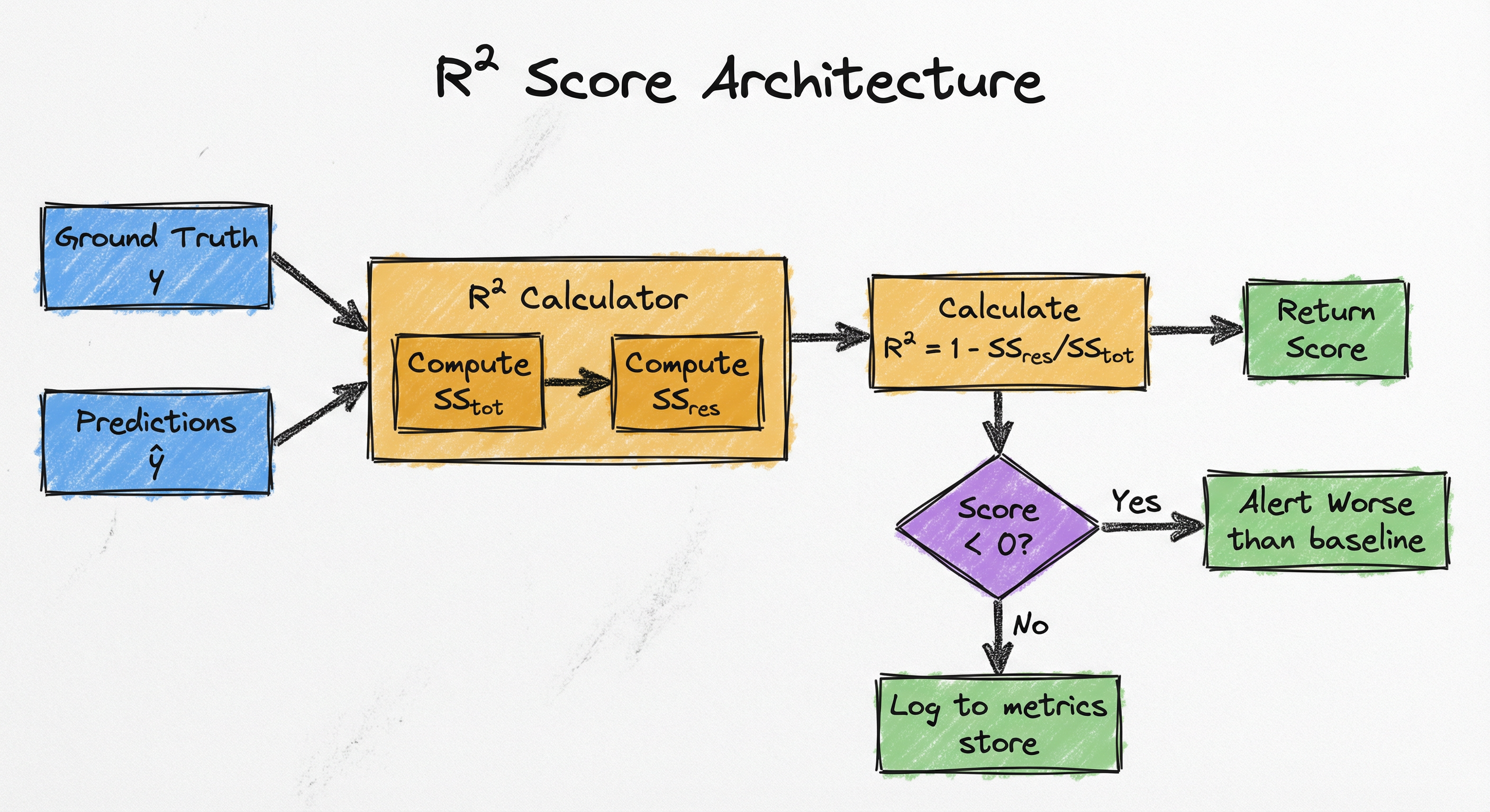
Data Flow
Step 1: Predictions (ŷ) and ground truth (y) arrays enter the scorer. Step 2: Input validation checks for shape compatibility and data quality. Step 3: Mean of y is computed. Step 4: SS_tot is computed from (y - mean) squared deviations. Step 5: SS_res is computed from (y - ŷ) squared deviations. Step 6: R² is calculated as 1 - (SS_res / SS_tot). Step 7: Optional post-processing (e.g., replacing special values if force_finite=True). Step 8: Score is returned, logged to experiment tracking, or triggers alerts if below threshold.
A linear flow showing ground truth and predictions feeding into an R² calculator, which computes SS_tot and SS_res in parallel, then combines them to produce the final R² score. A conditional branch checks if the score is negative and routes to an alert system if so.
How to Implement
Standard Libraries and Tools
Implementing R² score is straightforward in any language with basic array operations. In the Python ML ecosystem, scikit-learn provides the canonical implementation via sklearn.metrics.r2_score(). For statistical analysis with hypothesis testing and detailed model summaries, statsmodels includes R² (and adjusted R²) as part of its regression output.
Key Implementation Considerations
1. Handling edge cases: What happens when y is constant (zero variance)? SS_tot becomes zero, causing division by zero. Scikit-learn's force_finite=True (default) maps this to 1.0 if predictions are perfect, 0.0 otherwise.
2. Multi-output regression: When predicting multiple targets simultaneously (e.g., predicting both [latitude, longitude] for location estimation), you need to decide how to aggregate per-target R² scores. Options include uniform averaging (mean of all R² values) or variance-weighted averaging (weight each R² by that target's variance).
3. Sample weights: If some samples are more important than others (e.g., recent data in time series), you can compute weighted R² by passing sample_weight to the scorer.
4. Adjusted R² computation: Scikit-learn does not provide adjusted R² directly. You must compute it manually using the formula that incorporates the number of features.
Cost Note: For a real-time prediction API serving 10,000 requests per second (like a Razorpay fraud scoring endpoint), computing R² on every request is wasteful. Instead, log predictions and ground truth to a data warehouse, and compute R² in batch (hourly or daily) as part of your model monitoring pipeline.
from sklearn.metrics import r2_score
import numpy as np

# Ground truth and predictions
y_true = np.array([3.5, 2.1, 7.8, 4.2, 5.9])
y_pred = np.array([3.2, 2.4, 7.5, 4.0, 6.1])

# Compute R² score
r2 = r2_score(y_true, y_pred)
print(f"R² Score: {r2:.4f}")  # Output: R² Score: 0.9821

# Interpretation: 98.21% of variance is explained by the model
This is the simplest use case: two 1D arrays of equal length. The function returns a single float representing the coefficient of determination. An R² of 0.9821 indicates excellent fit — nearly all variance is explained.
from sklearn.metrics import r2_score
import numpy as np

def adjusted_r2(y_true, y_pred, n_features):
    """
    Calculate adjusted R² to account for model complexity.

    Args:
        y_true: Ground truth values
        y_pred: Predicted values
        n_features: Number of predictor variables (excluding intercept)

    Returns:
        Adjusted R² score
    """
    n = len(y_true)
    r2 = r2_score(y_true, y_pred)
    adj_r2 = 1 - (1 - r2) * (n - 1) / (n - n_features - 1)
    return adj_r2

# Example: comparing two models
y_true = np.random.randn(100) + 5
y_pred_simple = y_true + np.random.randn(100) * 0.5  # 1 feature
y_pred_complex = y_true + np.random.randn(100) * 0.6  # 10 features

print(f"Simple model R²: {r2_score(y_true, y_pred_simple):.4f}")
print(f"Simple model Adj R²: {adjusted_r2(y_true, y_pred_simple, 1):.4f}")

print(f"Complex model R²: {r2_score(y_true, y_pred_complex):.4f}")
print(f"Complex model Adj R²: {adjusted_r2(y_true, y_pred_complex, 10):.4f}")

# The complex model may have similar R² but lower adjusted R²
# due to the penalty for additional features
Adjusted R² penalizes models for adding features that don't meaningfully improve fit. This is critical during feature selection — if adding a feature increases R² slightly but decreases adjusted R², that feature is likely noise. The penalty factor (n-1)/(n-p-1) grows as p (number of features) approaches n (number of samples), preventing overfitting on small datasets.
from sklearn.metrics import r2_score
import numpy as np

# Multi-target regression: predicting [price, quantity] for inventory
y_true = np.array([
    [100, 50],   # item 1: ₹100, 50 units
    [200, 30],   # item 2: ₹200, 30 units
    [150, 45],   # item 3: ₹150, 45 units
    [180, 35],   # item 4: ₹180, 35 units
])

y_pred = np.array([
    [105, 48],
    [195, 32],
    [148, 46],
    [182, 34],
])

# Uniform average: mean of per-target R²
r2_uniform = r2_score(y_true, y_pred, multioutput='uniform_average')
print(f"R² (uniform avg): {r2_uniform:.4f}")

# Per-target R² scores
r2_per_target = r2_score(y_true, y_pred, multioutput='raw_values')
print(f"R² per target: {r2_per_target}")
print(f"  Price R²: {r2_per_target[0]:.4f}")
print(f"  Quantity R²: {r2_per_target[1]:.4f}")

# Variance-weighted: weight each target by its variance
r2_weighted = r2_score(y_true, y_pred, multioutput='variance_weighted')
print(f"R² (variance weighted): {r2_weighted:.4f}")
For multi-output regression, you need to decide how to aggregate per-target scores. uniform_average treats all targets equally (simple mean). variance_weighted gives more weight to targets with higher variance — useful when some targets vary more than others (e.g., price varies more than quantity in the above example). raw_values returns individual scores for diagnostic purposes.
from sklearn.linear_model import LinearRegression
from sklearn.metrics import r2_score
from sklearn.model_selection import train_test_split
import numpy as np

# Simulate a dataset with many noise features
np.random.seed(42)
X = np.random.randn(100, 50)  # 50 features, 100 samples
y = X[:, 0] * 2 + X[:, 1] * 3 + np.random.randn(100) * 0.5  # Only 2 features matter

# Split data
X_train, X_test, y_train, y_test = train_test_split(X, y, test_size=0.3, random_state=42)

# Train model
model = LinearRegression()
model.fit(X_train, y_train)

# Evaluate
train_r2 = r2_score(y_train, model.predict(X_train))
test_r2 = r2_score(y_test, model.predict(X_test))

print(f"Train R²: {train_r2:.4f}")
print(f"Test R²: {test_r2:.4f}")

if test_r2 < 0:
    print("⚠️  WARNING: Negative test R² indicates severe overfitting!")
    print("   The model performs worse than predicting the mean.")
    print("   Consider: regularization, feature selection, or more data.")
elif train_r2 - test_r2 > 0.1:
    print("⚠️  WARNING: Large train-test R² gap suggests overfitting.")
    print(f"   Gap: {train_r2 - test_r2:.4f}")
This example demonstrates a critical production pattern: always check test R². A high training R² with low or negative test R² is a classic overfitting signature. With 50 features and only 100 samples, the model memorizes training noise. In production, set up alerts when test R² drops below a threshold or when the train-test gap exceeds an acceptable margin (e.g., 0.1).
# Example configuration for R² monitoring in a production pipeline
# (YAML format for ML observability platform)

model_monitoring:
  metrics:
    - name: r2_score
      type: regression
      threshold: 0.75  # Alert if R² drops below 0.75
      compute_frequency: hourly
      sample_size: 10000  # Use 10K recent predictions

    - name: adjusted_r2
      type: regression
      n_features: 42
      threshold: 0.70
      compute_frequency: hourly

  alerts:
    - condition: "r2_score < 0"
      severity: critical
      message: "Negative R² detected - model worse than baseline"

    - condition: "train_r2 - test_r2 > 0.15"
      severity: warning
      message: "Large train-test R² gap - possible overfitting"

    - condition: "r2_score < 0.60 and previous_r2 > 0.75"
      severity: high
      message: "R² dropped significantly - model degradation detected"
Common Implementation Mistakes
- ●
Using R² as the sole evaluation metric for non-linear models: R² is mathematically valid for any regression model, but it's most interpretable for linear regression where the variance decomposition SS_tot = SS_reg + SS_res holds. For deep neural networks or gradient boosting models, R² can be misleading. Prefer MAE, RMSE, or domain-specific metrics alongside R².
- ●
Ignoring negative R² on test data: Negative test R² is not a bug — it's a critical signal that your model is worse than a constant baseline. This often indicates overfitting, feature leakage that doesn't generalize, or train-test distribution shift. Never ignore it.
- ●
Comparing R² across datasets with different variance: An R² of 0.80 on a high-variance dataset (where predictions are inherently difficult) may represent better modeling skill than an R² of 0.95 on a low-variance dataset. R² is scale-invariant but variance-dependent.
- ●
Adding features to maximize R² without checking adjusted R²: Standard R² never decreases when you add features, even if they're random noise. This makes it unsuitable for feature selection. Always use adjusted R² or cross-validated performance when comparing models with different numbers of features.
- ●
Assuming R² = r² for multiple regression: In simple linear regression (one predictor), R² equals the square of the correlation coefficient. This does NOT generalize to multiple regression. For multiple predictors, R² can be much higher than the squared correlation between any single predictor and the target.
When Should You Use This?
Use When
You need a scale-invariant metric that allows comparison across different datasets or domains (e.g., comparing a house price model to a temperature prediction model)
Stakeholders require an intuitive explanation of model quality — "explains 85% of variance" is easier to communicate than "MAE of 2.3 units"
You're performing feature selection or model comparison and want to know if added complexity (more features, deeper models) improves explanatory power beyond what you'd expect by chance (use adjusted R² in this case)
Your modeling objective is variance explanation rather than absolute error minimization — common in scientific research where understanding relationships matters more than prediction accuracy
You're working with linear or near-linear relationships where the variance decomposition SS_tot = SS_reg + SS_res is meaningful and interpretable
Avoid When
You're dealing with highly non-linear models (deep neural networks, complex ensembles) where the variance decomposition breaks down and R² loses its intuitive "variance explained" interpretation
Your application requires interpretability of errors in the original units — stakeholders care more about "predictions are off by ₹5,000 on average" (MAE) than "model explains 85% of variance"
The target variable has low inherent variance (e.g., binary outcomes like click/no-click, or nearly constant values) — R² becomes unstable or uninformative in these cases
You need to directly optimize a business metric — for example, in A/B testing conversion rate prediction, MAE on conversion rate may be more actionable than R²
You're comparing models trained on different subsets of data where the variance of y differs — R² comparisons become invalid because the denominators (SS_tot) are different
Key Tradeoffs
The Core Tradeoff: Intuition vs. Actionability
R²'s greatest strength is also its limitation: it's scale-invariant. You can compare an R² of 0.85 for predicting house prices to an R² of 0.85 for predicting delivery times — the metric is comparable across domains. But this abstraction comes at a cost: you lose information about the magnitude of errors.
A model with R² = 0.90 predicting house prices could have an MAE of ₹10 lakh (unacceptable for budget buyers) or ₹50,000 (excellent). The R² alone doesn't tell you which. In production, you almost always need R² alongside an absolute error metric like MAE or RMSE.
R² vs. Adjusted R²: The Feature Selection Dilemma
Standard R² suffers from a fatal flaw in feature selection: it never decreases when you add features, even if those features are pure noise. Add 100 random columns to your dataset, and R² will stay the same or (likely) increase slightly just by chance.
Adjusted R² fixes this by penalizing model complexity. The penalty grows as the ratio of features to samples increases. But adjusted R² introduces a new tradeoff: it's dataset-size dependent. With 10,000 samples, the penalty for 50 features is negligible. With 100 samples and 50 features, the penalty is severe. This makes adjusted R² hard to compare across datasets of different sizes.
Recommendation: Use adjusted R² for within-dataset feature selection. Use cross-validated MAE or RMSE for comparing models across datasets.
When Negative R² is Actually Informative
Negative test R² is often treated as a failure, but it's actually providing valuable information: your model has overfit so badly that it's worse than predicting the mean. This is a stronger signal than a mediocre positive R² like 0.2, which might just indicate a hard problem. Negative R² is an actionable alert: regularize, simplify, or collect more data.
| Metric | Strength | Weakness |
|---|---|---|
| R² | Scale-invariant, intuitive "variance explained" interpretation | Insensitive to error magnitude, always increases with features |
| Adjusted R² | Penalizes complexity, suitable for feature selection | Dataset-size dependent, requires knowing number of features |
| MAE | Interpretable in original units, robust to outliers | Not scale-invariant, can't compare across domains |
| RMSE | Penalizes large errors more than MAE | Sensitive to outliers, less interpretable than MAE |
Alternatives & Comparisons
MAE measures average absolute prediction error in the original units of the target variable. Use MAE when stakeholders need errors in interpretable units ("off by ₹5,000 on average") rather than variance explained. MAE is also more robust to outliers than R², which heavily penalizes large errors through the squared residuals.
RMSE is the square root of MSE and shares the same units as the target variable, making it interpretable like MAE but with heavier penalties for large errors. Use RMSE when large errors are disproportionately costly (e.g., wildly wrong delivery time predictions that cause customer churn). R² can be derived from MSE: R² = 1 - (MSE / Var(y)).
MAPE expresses error as a percentage of actual values, making it scale-invariant like R² but in a different way. Use MAPE when relative error matters more than absolute error (e.g., predicting sales where a ₹1 lakh error on a ₹10 lakh product is worse than a ₹1 lakh error on a ₹1 crore product). However, MAPE breaks down when actual values are near zero.
Residual plots visualize the distribution of errors, revealing patterns that scalar metrics like R² miss (e.g., heteroscedasticity, non-linearity, outliers). Use residual plots for diagnostic analysis alongside R² — a high R² with patterned residuals indicates model misspecification (e.g., fitting a linear model to non-linear data).
Pros, Cons & Tradeoffs
Advantages
Scale-invariant and domain-agnostic: Allows meaningful comparison of model quality across different prediction tasks and units of measurement — an R² of 0.85 has the same interpretation whether predicting temperature in Celsius or house prices in INR.
Intuitive interpretation for stakeholders: "The model explains 85% of the variance" is much easier for non-technical audiences to understand than "MAE is 2.3 units" or "RMSE is 5.1 units."
Detects overfitting through negative values: Negative R² on test data is an unambiguous signal that the model is worse than a constant baseline — a critical diagnostic that error metrics like MAE cannot provide.
Computationally trivial: complexity makes it suitable for real-time monitoring dashboards, A/B testing platforms, and high-frequency model evaluation pipelines.
Adjusted R² enables principled feature selection: Unlike standard R², adjusted R² penalizes unnecessary features, making it a valid metric for comparing models with different levels of complexity on the same dataset.
Connects to statistical theory: For linear models, R² is tied to F-statistics, ANOVA, and hypothesis testing frameworks, making it essential for statistical inference and model diagnostics in scientific research.
Disadvantages
Loses magnitude information: An R² of 0.90 could correspond to an MAE of ₹1,000 or ₹10 lakh depending on the scale of the target variable — the metric alone doesn't tell you if errors are acceptable for your use case.
Always increases (or stays constant) with added features: Standard R² cannot detect when you've added useless features — it will never decrease, even if you add 100 random noise columns. This makes it unsuitable for feature selection without using the adjusted variant.
Misleading for non-linear models: The variance decomposition (SS_tot = SS_reg + SS_res) only holds for linear models with intercepts. For non-linear models, R² can be computed but loses its "variance explained" interpretation and can behave unexpectedly.
Sensitive to outliers: Because R² uses squared residuals (inherited from SS_res), a few large outliers can dramatically lower the score, even if the model performs well on the majority of samples. MAE is more robust in this regard.
Not comparable across datasets with different variance: An R² of 0.60 on a high-variance dataset may represent better modeling than an R² of 0.85 on a low-variance dataset. The metric is only meaningful when the inherent predictability of the target is considered.
Can be negative on test data, confusing stakeholders: While negative R² is informative to ML practitioners, explaining to a product manager that "negative is possible and means worse than baseline" can be confusing compared to always-positive metrics like MAE.
Failure Modes & Debugging
Negative R² on test data due to overfitting
Cause
Model learns noise patterns in training data that don't generalize to test data. With many features relative to samples (high p/n ratio), the model fits training residuals perfectly but makes predictions worse than the mean on unseen data.
Symptoms
High R² on training set (e.g., 0.95) but negative or very low R² on validation/test set (e.g., -0.3 or 0.1). Large gap between train and test performance. Predictions on test data have higher MSE than simply predicting the mean.
Mitigation
Apply regularization (Ridge, Lasso, or Elastic Net) to penalize large coefficients. Perform feature selection to remove low-importance features. Use cross-validation during training to detect overfitting earlier. Increase training data if possible. Monitor adjusted R² during feature engineering to catch complexity inflation.
Misleading high R² on low-variance targets
Cause
When the target variable has very low variance (e.g., predicting nearly constant values, or binary outcomes), even a naive model can achieve high R² because SS_tot is small. A model predicting constant values near the mean gets high R² by default.
Symptoms
R² above 0.90 but predictions cluster tightly around the mean. Low absolute MAE or RMSE relative to the scale, but predictions lack variation. The model has learned to predict nearly constant values.
Mitigation
Always examine the distribution of predictions alongside R². Check if predictions have similar variance to the target variable. Use residual plots to detect constant or near-constant predictions. Consider alternative metrics like MAE in absolute units, or domain-specific metrics that penalize lack of prediction diversity.
Incorrect interpretation for non-linear models
Cause
For non-linear models (or linear models without intercepts), the variance decomposition SS_tot = SS_reg + SS_res does not hold. R² can still be computed, but it no longer represents "proportion of variance explained" in the strict statistical sense.
Symptoms
R² behaves unexpectedly — for example, values exceeding 1.0 (impossible for linear regression with intercept) or wildly oscillating values across similar test sets. Adjusted R² calculated using the standard formula gives nonsensical results.
Mitigation
For non-linear models (random forests, neural networks, gradient boosting), treat R² as a benchmark comparison metric rather than "variance explained." Prefer MAE, RMSE, or MAPE for primary evaluation. When reporting R², add a disclaimer that the "variance explained" interpretation is approximate for non-linear models.
Feature proliferation inflating R² without improving generalization
Cause
Standard R² never decreases when features are added, even if the new features are pure noise. Engineers add features to maximize R², unknowingly overfitting to training data noise.
Symptoms
R² steadily increases as features are added during feature engineering. Training R² reaches very high values (>0.95) but test R² plateaus or decreases. Model becomes complex and slow to train without meaningful performance gains.
Mitigation
Use adjusted R² instead of standard R² for feature selection — it penalizes added features unless they improve fit beyond chance. Perform forward/backward stepwise selection or L1 regularization (Lasso) to automate feature pruning. Track both train and test R² in parallel, and stop adding features when test R² stops improving.
Comparing R² across datasets with different inherent variance
Cause
R² is calculated relative to the variance in the target variable (SS_tot). A dataset with high inherent variance (hard to predict) and R² = 0.70 may represent better modeling skill than a low-variance dataset (easy to predict) with R² = 0.90.
Symptoms
Model A has R² = 0.65 on a complex, noisy dataset (e.g., stock price prediction). Model B has R² = 0.92 on a simple, stable dataset (e.g., predicting daylight hours from date). Stakeholders incorrectly conclude Model B is "better."
Mitigation
Never compare R² across datasets with different targets or variance structures. When comparing models, use the same test set. Report R² alongside the variance of the target variable (Var(y)) to provide context. Consider using standardized metrics like MAE/mean(y) or RMSE/std(y) for cross-dataset comparisons.
Outliers disproportionately impacting R² due to squared residuals
Cause
R² uses squared residuals (SS_res = Σ(y - ŷ)²), which heavily penalizes large errors. A few extreme outliers can dominate the residual sum of squares, causing R² to drop dramatically even if the model performs well on the majority of samples.
Symptoms
R² is much lower than expected based on visual inspection of predictions vs. actuals. Removing a small number of extreme data points causes R² to jump significantly (e.g., from 0.60 to 0.85). MAE (which uses absolute errors) is reasonably good, but R² is poor.
Mitigation
Examine residual distributions and identify outliers using plots or statistical tests (e.g., points with |residual| > 3σ). Decide whether outliers are genuine data (requiring robust models) or errors (requiring cleaning). Use robust regression techniques (Huber loss, quantile regression) if outliers are inherent to the domain. Report MAE alongside R² for a more complete picture.
Placement in an ML System
Where R² Fits in the ML Pipeline
R² score is primarily used during the model evaluation and selection phase, but its role extends across the ML lifecycle:
1. Training Phase: Computed on validation sets during hyperparameter tuning (e.g., grid search with cross-validation). Helps select the best model configuration before test set evaluation.
2. Model Selection Phase: Used to compare multiple model families (linear regression vs. random forest vs. gradient boosting) on the held-out test set. Often reported alongside MAE and RMSE for a complete picture.
3. Production Monitoring Phase: Logged periodically (hourly/daily) to detect model degradation. A sudden drop in R² can indicate data drift, training-serving skew, or changing user behavior.
4. A/B Testing Phase: When deploying a new model variant, R² on live traffic helps quantify whether the new model explains more variance in real-world outcomes. This is distinct from business metrics (revenue, engagement) but provides early technical signals.
Upstream Dependencies
R² requires ground truth labels, which can introduce latency in production systems. For example, in a delivery time prediction model (Swiggy/Zomato), you predict delivery time at order placement, but the true delivery time is only known 30-60 minutes later. This means R² can only be computed with a delay, requiring asynchronous pipelines that join predictions with delayed ground truth.
Downstream Impact
R² often gates deployment decisions: "Only deploy if test R² > 0.80" or "Retrain weekly and deploy only if new R² exceeds old R² by 0.03." These thresholds should be set based on business impact analysis, not arbitrary statistical benchmarks.
Production Pattern: For regression APIs at scale, compute R² in batch (hourly/daily) on sampled predictions rather than per-request. Store predictions + ground truth in a data warehouse, then run a scheduled job to compute metrics and alert on degradation.
Pipeline Stage
Evaluation / Validation
Upstream
- Model Training
- Hyperparameter Tuning
- Cross-Validation
Downstream
- Model Selection
- Production Deployment
- A/B Testing Framework
Scaling Bottlenecks
R² computation is and extremely lightweight — even for millions of predictions, it takes milliseconds. The bottleneck is not computation but data collection and logging. In a high-throughput prediction API (e.g., Razorpay's fraud scoring serving 10K QPS), logging every prediction and ground truth to compute R² hourly can generate terabytes of data monthly. Use sampling (e.g., log 1% of predictions) or streaming aggregation (update running sums without storing raw data) to manage scale. For real-time dashboards, compute R² on recent windows (last hour, last day) using reservoir sampling or time-decay weighting.
Production Case Studies
Airbnb built a regression model to predict the market value of homes listed on their platform. They used R² (alongside MAE and RMSE) to evaluate model fit across different geographic markets. The team found that R² varied significantly by region — dense urban markets with diverse housing stock had lower R² (~0.65) compared to suburban markets with more uniform properties (~0.85). This geographic variance in R² informed how they set price suggestion confidence intervals.
The model achieved an overall R² of 0.72 across all markets. More importantly, the variance in R² across regions helped Airbnb identify where their feature set was incomplete (urban markets needed additional features like proximity to transit, walkability scores) and where simpler models sufficed.
Zillow's Zestimate model predicts home values using regression on hundreds of features (property characteristics, location, market trends). They report median absolute error publicly, but internally use R² to assess model quality across different housing markets. In markets with high volatility (e.g., tech hubs during boom/bust cycles), R² tends to be lower (~0.60-0.70) compared to stable markets (~0.80-0.90). Zillow uses adjusted R² to prevent feature engineering teams from adding low-value features just to inflate standard R².
Zillow's median absolute error is approximately 2% for on-market homes and 7% for off-market homes. The R² varies by market type but averaging around 0.70-0.80 for on-market properties, indicating strong explanatory power despite inherent market unpredictability.
Uber uses regression models to forecast demand (number of ride requests) at different times and locations. They evaluate models using R² to understand how much of the demand variance can be explained by features like time of day, day of week, weather, events, and historical trends. During model development, they discovered that R² for short-term forecasts (next 15 minutes) was much higher (~0.90) than long-term forecasts (next 4 hours, R² ~0.60), which informed their decision to use different model architectures for different forecast horizons.
Short-term demand forecasts achieved R² > 0.85, enabling efficient driver allocation and surge pricing. The R² metric helped the team identify when they'd hit the ceiling of what their feature set could explain, prompting investment in external data sources (traffic, public transit schedules) to capture additional variance.
PhonePe built a real-time transaction model for fraud prevention, processing over 2.5 billion transactions monthly. The ML-based system uses regression models and classification techniques to detect fraudulent patterns while maintaining millisecond-level response times.
PhonePe's ML fraud detection system segments transactions using customer demography, behavioral variables, and historical patterns to reduce false positives. The system leverages real-time variables through their Yoda knowledge store and employs graph-based detection for coordinated fraud clusters.
Tooling & Ecosystem
The canonical Python implementation of R² score via sklearn.metrics.r2_score(). Supports multi-output regression, sample weighting, and the force_finite parameter to handle edge cases (constant y values). Integrates seamlessly with scikit-learn's cross-validation and model selection utilities.
Statistical modeling library that reports both R² and adjusted R² in regression summaries. Includes hypothesis testing, confidence intervals, and diagnostic plots alongside coefficient of determination. Best for statistical inference rather than pure prediction.
Provides tf.keras.metrics.R2Score as a built-in metric for regression models. Can be used during training as a monitored metric or computed post-hoc on predictions. Supports streaming computation for large datasets that don't fit in memory.
Part of the TorchMetrics library. Offers R2Score as a differentiable metric that can be computed during training or validation. Handles batched computation and multi-device aggregation in distributed training setups.
Distributed implementation via RegressionEvaluator with metric='r2'. Designed for large-scale regression evaluation on datasets that don't fit on a single machine. Computes R² across partitions using distributed aggregation.
The summary.lm() function in base R reports both R² and adjusted R² for linear models. R's statistical heritage makes it the gold standard for detailed model diagnostics, ANOVA decomposition, and hypothesis testing around coefficient of determination.
Experiment tracking platform that automatically logs R² (and adjusted R²) when using scikit-learn models. Provides visualization dashboards to compare R² across runs, hyperparameter settings, and model versions. Integrates with production deployment pipelines.
Research & References
Chicco, D., Warrens, M. J., & Jurman, G. (2021)PeerJ Computer Science
Empirical study demonstrating that R² provides more informative model comparisons than absolute error metrics across diverse regression tasks, though it should be used alongside domain-specific metrics.
Spiess, A. N., & Neumeyer, N. (2010)BMC Pharmacology
Monte Carlo simulation study showing that R² can be misleading for non-linear regression models because the variance decomposition SS_tot = SS_reg + SS_res no longer holds, recommending AIC/BIC for non-linear model comparison.
Nakagawa, S., Johnson, P. C., & Schielzeth, H. (2017)Journal of The Royal Society Interface
Extends the concept of R² to generalized linear mixed models (GLMMs), proposing marginal R² (variance explained by fixed effects) and conditional R² (variance explained by fixed and random effects).
Zhang, Y., Chen, H., & Wang, L. (2024)arXiv preprint
Identifies inconsistencies in R² implementations across Python (scikit-learn), R, and Julia, particularly in handling edge cases like constant targets and multi-output regression, emphasizing the need for standardization.
Renaud, O., & Victoria-Feser, M. P. (2010)Journal of the American Statistical Association
Proposes a robust version of R² that is less sensitive to outliers by replacing squared residuals with a bounded loss function, improving reliability in the presence of contaminated data.
Interview & Evaluation Perspective
Common Interview Questions
- ●
What does an R² of 0.85 mean in practical terms?
- ●
Can R² be negative? If so, what does that indicate?
- ●
How does R² differ from the correlation coefficient (r)?
- ●
When should you use adjusted R² instead of standard R²?
- ●
Why is R² not suitable as the sole metric for evaluating non-linear models?
- ●
How would you interpret an R² of 0.40 — is that good or bad?
Key Points to Mention
- ●
R² measures proportion of variance explained, not absolute error — it's a relative metric benchmarked against predicting the mean.
- ●
R² can be negative on test data, which indicates the model performs worse than a naive baseline that always predicts the mean. This is a critical overfitting signal.
- ●
For simple linear regression, R² equals r² (square of correlation), but this equivalence does NOT hold for multiple regression or non-linear models.
- ●
Adjusted R² penalizes added features and should be used for feature selection or model comparison when models have different numbers of parameters.
- ●
R² is scale-invariant but variance-dependent — you can compare R² across different units (₹ vs. kg) but not across datasets with different inherent variance.
- ●
Always use R² alongside MAE or RMSE in production — R² tells you percentage of variance explained, but absolute error metrics tell you if errors are acceptable in real-world units.
Pitfalls to Avoid
- ●
Claiming R² "measures accuracy" — it measures variance explained, which is conceptually different from prediction accuracy (measured by MAE/RMSE).
- ●
Assuming higher R² always means a better model — an R² of 0.90 on a low-variance dataset may be less impressive than 0.70 on a high-variance dataset.
- ●
Using standard R² for feature selection without considering adjusted R² — standard R² never decreases when you add features, even if they're noise.
- ●
Comparing R² across different test sets or datasets — the metric is only meaningful when evaluated on the same data because the denominator (SS_tot) depends on the variance of y.
- ●
Ignoring negative R² as a "bug" — it's actually valuable diagnostic information indicating your model has overfit or learned non-generalizable patterns.
Senior-Level Expectation
A senior candidate should be able to articulate when R² is appropriate and when it's misleading. They should explain the mathematical relationship to variance decomposition (SS_tot = SS_reg + SS_res for linear models), discuss why this breaks down for non-linear models, and propose complementary metrics (MAE, RMSE, residual analysis) for a complete evaluation. They should also discuss production considerations: how to compute R² efficiently on streaming data, when to use adjusted R² vs. cross-validation for model selection, and how to set meaningful R² thresholds based on business impact rather than arbitrary statistical benchmarks. Finally, they should recognize that R² is a diagnostic tool, not an optimization target — directly optimizing for R² can lead to overfitting, and the real objective is often minimizing business cost (e.g., cost of prediction errors in revenue terms).
Summary
Let's bring it all together.
R² score (coefficient of determination) is a regression evaluation metric that quantifies the proportion of variance in the target variable that your model can explain. It's calculated as , where SS_res is the residual sum of squares (your model's errors) and SS_tot is the total variance (errors if you just predicted the mean).
The metric ranges from negative infinity to 1.0. A score of 1.0 is perfect, 0.0 means you're no better than predicting the mean, and negative values mean you're worse than that naive baseline — a critical overfitting signal that should trigger immediate investigation.
R² is scale-invariant, making it useful for comparing model quality across different domains and units. An R² of 0.85 for predicting house prices in INR has the same interpretation as 0.85 for predicting delivery times in minutes: the model explains 85% of the variance. But this abstraction comes at a cost — R² doesn't tell you the magnitude of errors in real-world units. You must pair it with MAE or RMSE for actionable insights.
For linear regression, R² has a clean "variance explained" interpretation because the decomposition SS_tot = SS_reg + SS_res holds exactly. For non-linear models, you can still compute R², but it loses this strict interpretation and can behave unexpectedly. In those cases, treat it as a benchmark metric rather than a fundamental measure of fit.
Adjusted R² solves a critical flaw: standard R² never decreases when you add features, even if they're noise. Adjusted R² penalizes complexity, making it essential for feature selection and model comparison when architectures differ in the number of parameters. The penalty grows as the ratio of features to samples increases, preventing overfitting on small datasets.
In production ML systems — from Airbnb's home value predictions to Uber's demand forecasts — R² serves multiple roles: model selection (choose the architecture with highest test R²), monitoring (alert when R² drops below threshold, signaling model degradation), and stakeholder communication ("the model explains 78% of variance" is more intuitive than "MAE is 2.3 units").
The key is knowing its limitations. Don't use R² as your sole metric. Don't compare it across different test sets. Don't ignore negative values — they're red flags, not bugs. And always ask: does this R² translate to acceptable prediction errors for my use case?
Final takeaway: R² measures how much of the variation in your outcome you've successfully modeled. It's a powerful diagnostic and communication tool, but it's fundamentally a variance metric, not an accuracy metric. Use it to understand how well you're capturing signal, but always validate that captured signal translates to real-world performance using absolute error metrics.