Hit Rate in Machine Learning
Here is the simplest question you can ask about a retrieval system: did it find anything useful?
Not how many useful things it found. Not where the useful thing appeared in the list. Just: yes or no, was there at least one relevant result in the top K?
That is exactly what Hit Rate (also called Hit Rate@K or HR@K) measures. For each query, it checks whether at least one relevant item appears in the retrieved top-K results. If yes, score = 1. If no, score = 0. Average across all queries, and you have the system-level Hit Rate.
This deceptive simplicity is precisely what makes Hit Rate so useful. It is the most intuitive retrieval metric: even a product manager who has never heard of NDCG or MAP can understand "78% of queries returned at least one good result." It strips away nuances about ranking position and relevance gradation, cutting straight to the core question of whether the system works at all.
Hit Rate dominates evaluation in two specific areas: candidate retrieval (the first stage of a multi-stage ranking pipeline, where you just need the right items in the pool) and recommendation systems (where a user seeing at least one relevant recommendation counts as a success). It is also increasingly used in RAG pipelines to evaluate whether the retrieval step surfaces at least one document that contains the answer. If you are building any system that retrieves items from a large corpus and feeds them into a downstream ranker or LLM, Hit Rate is probably the first metric you should track.
Concept Snapshot
- What It Is
- A binary retrieval metric that measures the fraction of queries for which at least one relevant item appears in the top-K retrieved results.
- Category
- Evaluation
- Complexity
- Beginner
- Inputs / Outputs
- Inputs: a set of queries, each with a top-K retrieved result list and a set of known relevant items. Output: a single score between 0 and 1 representing the fraction of queries with at least one hit.
- System Placement
- Used to evaluate the first-stage retrieval (candidate generation) in recommendation and search pipelines, and increasingly for RAG retrieval evaluation. Typically computed offline during model evaluation and online in A/B tests.
- Also Known As
- HR@K, Hit Rate at K, Hit Ratio, Success Rate, Success@K, Recall@1 (when K=1 and one relevant item)
- Typical Users
- ML engineers, recommendation system developers, search engineers, RAG pipeline builders, data scientists
- Prerequisites
- Basic set operations (intersection), Understanding of retrieval systems, Concept of relevance labels, Top-K retrieval
- Key Terms
- HR@Ktop-K retrievalbinary successcandidate retrievalrelevant itemhitmissretrieval recall
Why This Concept Exists
The Problem: Evaluating Whether Retrieval Works at All
In a multi-stage retrieval and ranking pipeline -- the architecture used by virtually every production search and recommendation system -- the first stage (candidate generation) has a very specific job: cast a wide net and make sure the relevant items are in the candidate pool. If a relevant item never enters the candidate pool, no amount of sophisticated re-ranking downstream can save it.
Consider how a recommendation system like Flipkart's product feed works. You have 500 million products. The user opens the app. The first-stage retriever (often an approximate nearest-neighbor search) narrows this down to maybe 1000 candidates. Then a second-stage ranker (a LightGBM or neural model) re-ranks those 1000 into a final list of 20 items shown to the user.
The critical question for the first stage is not "did you rank the best item at position 1?" -- that's the re-ranker's job. The question is: "Is the best item somewhere in your 1000 candidates?" Hit Rate answers exactly this question.
Why Not Just Use Recall@K?
Recall@K measures what fraction of all relevant items appear in the top-K. If there are 50 relevant items and your top-K contains 10 of them, Recall@K = 10/50 = 0.20. This is useful, but it conflates two different problems:
- Queries where the system found some but not all relevant items (partial success)
- Queries where the system found nothing relevant (complete failure)
Hit Rate separates these cleanly. A query with 10 out of 50 relevant items in the top-K is a hit (score = 1). A query with 0 out of 50 is a miss (score = 0). This binary framing answers the most fundamental question: does the retrieval stage work for this query, yes or no?
The Rise of RAG and Hit Rate's Renewed Importance
With the explosion of Retrieval-Augmented Generation (RAG) systems since 2023, Hit Rate has found a new and critical use case. In a RAG pipeline, you retrieve K documents and feed them to an LLM. The LLM can only answer correctly if at least one retrieved document contains the relevant information. It doesn't matter if you retrieved 3 relevant documents or 1 -- the LLM only needs one good document to generate a correct answer.
This makes Hit Rate a near-perfect proxy for RAG retrieval quality. If Hit Rate@5 is 0.90, that means 90% of queries will have at least one relevant document in the LLM's context window. The remaining 10% are queries where the retrieval stage failed entirely, and no prompt engineering can compensate.
Key Insight: Hit Rate exists because the most fundamental question about any retrieval system is binary: did it work or didn't it? Before worrying about ranking quality (NDCG) or coverage (Recall@K), you need to know what fraction of queries have any chance of success at all.
Core Intuition & Mental Model
The Cache Hit Analogy
The best way to understand Hit Rate is through the analogy of a cache hit rate in computer systems. When your application requests data from a cache:
- Cache hit: The data is in the cache. Success.
- Cache miss: The data is not in the cache. Failure. Must go to the slow database.
- Cache hit rate: The fraction of requests that resulted in a hit.
Hit Rate@K in retrieval is the exact same concept. For each query:
- Hit: At least one relevant item is in the top-K results. The downstream system (ranker, LLM) has something to work with.
- Miss: No relevant item is in the top-K. The downstream system is doomed to fail, no matter how good it is.
- Hit Rate@K: The fraction of queries that resulted in a hit.
Just as a cache hit rate of 95% means 5% of requests take the slow path, a Hit Rate@K of 0.95 means 5% of queries have no relevant results in their candidate pool -- and those queries are unsalvageable downstream.
Why Binary Is Powerful
You might think a binary metric is too crude. But consider this: in many real-world systems, the difference between "one relevant item in top-K" and "zero relevant items in top-K" is the single largest quality cliff. Going from 0 to 1 relevant item is transformative (the system goes from broken to functional). Going from 1 to 5 relevant items is incremental improvement.
This is especially true in:
- RAG pipelines: The LLM needs at least one good document. Having three instead of one might marginally improve answer quality, but having zero is catastrophic.
- Candidate retrieval: If the right product is not in the candidate pool, it will never be shown to the user. Whether the pool has 1 or 10 copies of "right" products matters much less than whether it has any.
- Navigational queries: When a user searches for "Zerodha Kite login," there is exactly one right answer. Either you have it or you don't.
The Threshold Perspective
Another way to think about Hit Rate: it is Recall@K with a threshold of 1. Instead of measuring the fraction of relevant items retrieved, you're just asking "is the fraction greater than zero?" This threshold transforms a continuous metric into a binary one, which is often exactly what you need for operational decisions: is the retrieval pipeline meeting the minimum bar, or is it completely failing for some queries?
Technical Foundations
Mathematical Definition
Let be a set of queries. For each query , let:
- = the set of top-K items retrieved by the system
- = the set of ground-truth relevant items for query
The Hit Rate at K (HR@K) for a single query is a binary indicator:
In plain language: if there is at least one item in both the retrieved set and the relevant set, it's a hit.
The system-level Hit Rate@K is the average over all queries:
Properties
- Range:
- Monotonicity in K: for all . Retrieving more items can only increase (or maintain) the hit rate -- you can never lose a hit by adding more results.
- Relation to Recall@K: For a single query with (one relevant item), is equivalent to .
- Relation to Precision@K: For a single query, iff .
- Position-unaware: Unlike NDCG or MRR, Hit Rate does not care where the relevant item appears within the top-K. Position 1 and position K contribute equally.
Worked Example
Consider 5 queries, each with a top-5 retrieved list. Relevant items are marked with a checkmark:
| Query | Position 1 | Position 2 | Position 3 | Position 4 | Position 5 | Hit? |
|---|---|---|---|---|---|---|
| irrelevant | relevant | irrelevant | irrelevant | relevant | 1 | |
| relevant | irrelevant | irrelevant | irrelevant | irrelevant | 1 | |
| irrelevant | irrelevant | irrelevant | irrelevant | irrelevant | 0 | |
| irrelevant | irrelevant | relevant | relevant | irrelevant | 1 | |
| irrelevant | irrelevant | irrelevant | irrelevant | irrelevant | 0 |
Interpretation: 60% of queries returned at least one relevant result in the top 5. Two queries ( and ) are complete misses.
HR@K at Different K Values
Notice how HR@K changes with K for the same example:
- HR@1 = 1/5 = 0.20 (only has a hit at position 1)
- HR@2 = 2/5 = 0.40 ( gets a hit at position 2)
- HR@3 = 3/5 = 0.60 ( gets a hit at position 3)
- HR@5 = 3/5 = 0.60 (no new hits at positions 4-5)
- HR@10 0.60 (could increase if relevant items exist at positions 6-10)
The curve of HR@K vs. K is non-decreasing and tells you how many results you need to retrieve to achieve a given hit rate. If HR@5 and HR@10 are very close, deeper retrieval isn't finding new relevant items.
Practical Note: The gap between HR@1 and HR@10 tells you about the distribution of relevant items across rank positions. A large gap means relevant items are scattered deep in the list -- your ranker might be struggling.
Internal Architecture
Hit Rate is a metric, not an infrastructure component, so its "architecture" describes how it's computed and integrated into ML evaluation pipelines. The computation is trivially simple; the interesting part is where Hit Rate fits into the broader system.
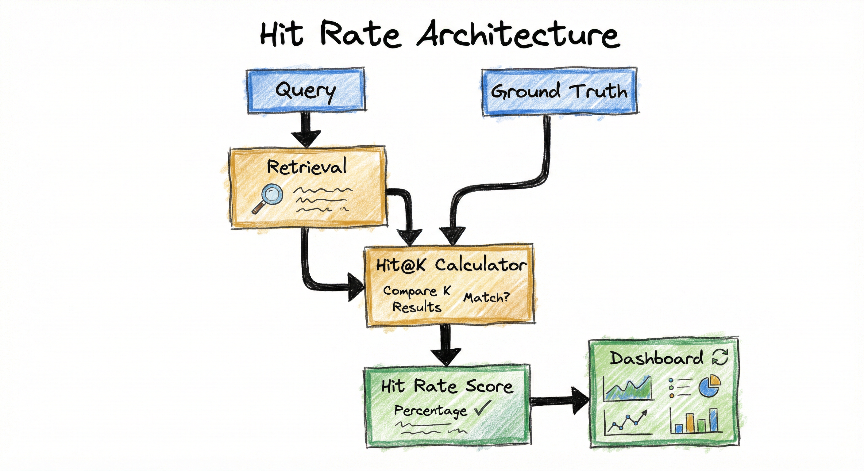
In a typical production pipeline, Hit Rate is computed in two contexts:
Offline evaluation: After training a new retrieval model (embedding model, ANN index, BM25 tuning), you run it on a test set of queries with known relevant items. HR@K is computed at various K values (10, 50, 100, 500) to determine whether the retrieval stage is surfacing candidates effectively. This runs in batch, often in a CI/CD pipeline.
Online A/B testing: When deploying a new retrieval model, you track HR@K on live traffic. For recommendation systems, "relevant" is defined post-hoc as items the user engaged with (clicked, purchased, watched). For search, it may be based on click-through or dwell time. Online HR@K tells you whether the new model is finding relevant items as well as the baseline.
Key Components
Retrieval System
The system under evaluation. Produces a ranked list of top-K items for each query. Could be an ANN index (FAISS, ScaNN), a BM25 search engine (Elasticsearch), a dense retriever (DPR, ColBERT), or a collaborative filtering model.
Ground Truth Labels
A mapping from queries to their known relevant items. Sources include human annotations, historical user interactions (purchases, clicks, bookmarks), or synthetic labels (for RAG, the documents known to contain the answer).
Hit Rate Calculator
For each query, checks whether the intersection of retrieved items and relevant items is non-empty. Returns 1 (hit) or 0 (miss). The simplest component -- just a set intersection and a boolean check.
Aggregation Layer
Averages hit/miss scores across all queries to produce the system-level HR@K. May also segment by query type (head vs. tail), category, or user cohort for deeper analysis.
Reporting & Alerting
Displays HR@K on dashboards, compares across model versions, and triggers alerts if HR@K drops below a threshold. In CI/CD, blocks deployment if HR@K regresses.
Data Flow
The data flow for Hit Rate computation is straightforward:
Step 1: For each query in the evaluation set, the retrieval system returns the top-K items: .
Step 2: Look up the ground-truth relevant items for this query.
Step 3: Compute the set intersection . If this is non-empty, record a hit (1); otherwise, a miss (0).
Step 4: Average across all queries to get .
Step 5: Report HR@K at multiple K values (e.g., K=1, 5, 10, 50, 100) to understand retrieval depth. Segment by query category if needed.
For online evaluation, Steps 1-4 happen on live traffic, with relevance determined by user actions (clicks, purchases) within a time window.
A directed flow from 'Query Set' to 'Retrieval System' to 'Top-K Results per Query'. Separately, 'Ground Truth Relevant Items' feeds into a 'Hit Rate Calculator' that also receives the 'Top-K Results'. The calculator outputs 'Hit or Miss per Query', which is aggregated into 'HR@K', feeding both a 'Dashboard / CI Pipeline' and an 'A/B Test Comparison'.
How to Implement
Implementation Is Almost Trivially Simple
Hit Rate is one of the easiest metrics to implement. The core computation is a set intersection followed by a boolean check. You can implement it in 5 lines of Python.
However, there are practical considerations that make real-world implementation more nuanced:
Choosing K: The right K depends on your pipeline. For candidate retrieval feeding a re-ranker, K might be 100-1000. For a RAG pipeline, K is typically 3-10 (the number of documents fed to the LLM). For a recommendation carousel, K is the number of visible items (6-20).
Defining relevance: This is the hard part. Binary relevance labels must come from somewhere -- human annotations, user interaction logs, or synthetic ground truth. The quality of your Hit Rate metric is only as good as your relevance labels.
Handling multiple relevant items: If a query has 50 relevant items and your top-K contains 3 of them, Hit Rate counts this as a perfect hit (1.0). If you care about how many relevant items you found, use Recall@K instead. Hit Rate is deliberately coarse-grained.
Cost Note: Computing Hit Rate is essentially free (set intersection on small sets). The expensive part is labeling relevance. For recommendation systems, you can use implicit feedback (purchases, clicks) at zero marginal labeling cost. For search and RAG, human annotation costs INR 30-80 per query-document pair. For 1000 queries with 10 candidates each = 10,000 labels, budget INR 3-8 lakh (9,500).
import numpy as np
from typing import List, Set

def hit_rate_at_k(
    retrieved: List[List[str]],
    relevant: List[Set[str]],
    k: int
) -> float:
    """Compute Hit Rate@K across multiple queries.

    Args:
        retrieved: List of retrieved item lists, one per query (ordered by rank).
        relevant: List of relevant item sets, one per query.
        k: Number of top results to consider.

    Returns:
        Hit Rate@K as a float between 0 and 1.
    """
    if len(retrieved) != len(relevant):
        raise ValueError("retrieved and relevant must have the same length")

    hits = 0
    for top_k_items, rel_items in zip(retrieved, relevant):
        # Take only the top-K items
        top_k_set = set(top_k_items[:k])
        # Check if there's at least one relevant item
        if top_k_set & rel_items:  # set intersection
            hits += 1

    return hits / len(retrieved) if retrieved else 0.0


# Example usage
retrieved_results = [
    ["doc_5", "doc_3", "doc_1", "doc_8", "doc_2"],  # Query 1
    ["doc_7", "doc_9", "doc_4", "doc_6", "doc_10"], # Query 2
    ["doc_1", "doc_2", "doc_3", "doc_4", "doc_5"],  # Query 3
    ["doc_11", "doc_12", "doc_13", "doc_14", "doc_15"], # Query 4
]

relevant_items = [
    {"doc_1", "doc_2"},          # Query 1: docs 1,2 are relevant
    {"doc_4"},                    # Query 2: doc 4 is relevant
    {"doc_99"},                   # Query 3: relevant doc not retrieved
    {"doc_20", "doc_21"},        # Query 4: relevant docs not retrieved
]

for k in [1, 3, 5]:
    hr = hit_rate_at_k(retrieved_results, relevant_items, k)
    print(f"HR@{k}: {hr:.3f}")
# Output:
# HR@1: 0.000  (no query has a hit at position 1)
# HR@3: 0.500  (queries 1 and 2 get hits by position 3)
# HR@5: 0.500  (no additional hits at positions 4-5)
This is the canonical Hit Rate implementation. For each query, we take the top-K retrieved items, form a set, and check for intersection with the relevant items set. The set intersection operator & returns a non-empty set (truthy) if there is at least one common element. We count hits and divide by the number of queries. Note that Hit Rate is position-unaware within the top-K -- it does not matter whether the hit is at position 1 or position K.
import numpy as np

def rag_hit_rate_at_k(
    questions: list[str],
    retrieved_contexts: list[list[str]],
    ground_truth_answers: list[str],
    k: int = 5
) -> float:
    """Compute hit rate for RAG retrieval.
    A 'hit' means at least one retrieved context contains
    a substring match with the ground truth answer.
    """
    hits = 0
    for question, contexts, answer in zip(
        questions, retrieved_contexts, ground_truth_answers
    ):
        answer_lower = answer.lower()
        if any(answer_lower in ctx.lower() for ctx in contexts[:k]):
            hits += 1
    return hits / len(questions) if questions else 0.0


# Evaluate RAG retrieval for an Indian e-commerce FAQ bot
questions = [
    "What is the return policy for electronics on Flipkart?",
    "How to track my Swiggy order?",
    "What is the GST rate for software services?",
    "How to link Aadhaar with PAN card?",
]

retrieved_contexts = [
    ["Flipkart offers a 10-day replacement policy for electronics...",
     "Electronics on Amazon India have a 30-day return window..."],
    ["Track your Zomato order in real-time from the app...",
     "Swiggy delivery tracking is available in the orders tab..."],
    ["Income tax slabs for FY 2025-26...",
     "Corporate tax rates in India..."],
    ["To link Aadhaar with PAN, visit the income tax e-filing portal...",
     "Aadhaar-PAN linking deadline extended to March 2026..."],
]

ground_truths = [
    "10-day replacement policy for electronics",
    "Swiggy delivery tracking is available in the orders tab",
    "18% GST rate for software services",
    "link Aadhaar with PAN",
]

hr = rag_hit_rate_at_k(questions, retrieved_contexts, ground_truths, k=3)
print(f"RAG Hit Rate@3: {hr:.2f}")
# Output: RAG Hit Rate@3: 0.75 (Query 3 misses -- no context mentions GST)
This example shows Hit Rate in a RAG context. The key difference from traditional retrieval is how 'relevance' is defined: a context is relevant if it contains the information needed to answer the question. The simple substring match shown here is a rough heuristic; in production, you would use semantic similarity or an LLM-as-judge approach (e.g., RAGAS ContextRecall). The insight is the same: if no retrieved context contains the answer, the LLM cannot generate a correct response.
import numpy as np

def recommendation_hit_rate(
    user_recs: dict[int, list[int]],
    user_interactions: dict[int, set[int]],
    k: int = 10
) -> dict:
    """Compute Hit Rate@K for a recommendation system."""
    hits = misses = 0
    for uid, recs in user_recs.items():
        if uid not in user_interactions:
            continue
        if set(recs[:k]) & user_interactions[uid]:
            hits += 1
        else:
            misses += 1
    total = hits + misses
    return {"hr_at_k": hits / total if total else 0.0, "hits": hits, "total": total}


# Simulate a Flipkart-like product recommendation evaluation
np.random.seed(42)
n_users, n_products = 1000, 50000

user_recs = {
    uid: list(np.random.choice(n_products, size=20, replace=False))
    for uid in range(n_users)
}
user_purchases = {
    uid: set(np.random.choice(n_products, size=np.random.randint(1, 6), replace=False))
    for uid in range(n_users)
}

for k in [1, 5, 10, 20]:
    r = recommendation_hit_rate(user_recs, user_purchases, k=k)
    print(f"HR@{k}: {r['hr_at_k']:.4f} ({r['hits']} hits / {r['total']} users)")
# A good production model achieves HR@10 of 0.15-0.40 depending on catalog size
This example evaluates Hit Rate for a recommendation system using implicit feedback (purchases). Each user has a set of items they interacted with (the ground truth) and a list of recommended items (the prediction). HR@K measures what fraction of users received at least one relevant recommendation in their top-K. This is the standard evaluation setup for collaborative filtering and content-based recommendation models. Note that with a large catalog (50K products), even a decent model may have relatively low HR@10 -- this is expected and the metric should be compared against baselines, not absolute thresholds.
import numpy as np
import faiss

def evaluate_faiss_hit_rate(
    query_embeddings: np.ndarray,
    index: faiss.Index,
    ground_truth: list[set[int]],
    k_values: list[int] = [1, 5, 10, 50, 100]
) -> dict[int, float]:
    """Evaluate Hit Rate at multiple K for a FAISS index."""
    max_k = max(k_values)
    distances, indices = index.search(query_embeddings, max_k)

    results = {}
    for k in k_values:
        hits = 0
        for retrieved_ids, rel_ids in zip(indices, ground_truth):
            if set(retrieved_ids[:k].tolist()) & rel_ids:
                hits += 1
        results[k] = hits / len(ground_truth)
    return results


# Build a FAISS IVF index and evaluate
dim, n_docs, n_queries = 768, 100_000, 500
np.random.seed(42)
doc_emb = np.random.randn(n_docs, dim).astype('float32')
q_emb = np.random.randn(n_queries, dim).astype('float32')

quantizer = faiss.IndexFlatL2(dim)
index = faiss.IndexIVFFlat(quantizer, dim, 100)
index.train(doc_emb)
index.add(doc_emb)
index.nprobe = 10

ground_truth = [
    set(np.random.choice(n_docs, size=np.random.randint(1, 4), replace=False))
    for _ in range(n_queries)
]

for k, hr in evaluate_faiss_hit_rate(q_emb, index, ground_truth).items():
    print(f"HR@{k:>3d}: {hr:.4f}")
# With a trained encoder, expect HR@1: 0.30-0.50, HR@10: 0.60-0.80, HR@100: 0.85-0.95
This demonstrates Hit Rate evaluation for a FAISS approximate nearest-neighbor index. The key optimization is batch search: query all at once with the maximum K, then compute HR at multiple K values from the same result set. The gap between exact search (IndexFlatL2) and approximate search (IndexIVFFlat) at the same HR@K tells you the cost of approximation.
# Hit Rate evaluation config (YAML)
evaluation:
  metric: hit_rate
  k_values: [1, 5, 10, 20, 50, 100]

  # Relevance definition
  relevance:
    source: implicit  # or 'explicit' for human labels
    interaction_types:
      - purchase
      - add_to_cart
      - click_with_dwell_time_gt_30s
    min_interactions: 1  # minimum interactions to count as relevant

  # Segmentation
  segments:
    - name: head_queries     # top 10% by frequency
      filter: query_freq >= p90
    - name: tail_queries     # bottom 50% by frequency
      filter: query_freq < p50
    - name: new_users
      filter: user_age_days < 7
    - name: power_users
      filter: user_interactions > 100

  # Alerting
  thresholds:
    hr_at_10_min: 0.70      # Alert if HR@10 drops below 70%
    hr_at_100_min: 0.90     # Alert if HR@100 drops below 90%
    regression_pct: 0.02    # Alert if HR drops by more than 2%
Common Implementation Mistakes
- ●
Confusing Hit Rate with Precision@K: Hit Rate is binary per query (hit or miss). Precision@K counts the fraction of retrieved items that are relevant. They answer fundamentally different questions: "Did we find anything?" vs. "How much of what we found is useful?" A query with 1 relevant item in top-10 has HR@10 = 1.0 but Precision@10 = 0.1.
- ●
Using Hit Rate alone for ranking quality: Hit Rate ignores position. A system that puts the relevant item at position K (last) gets the same score as one that puts it at position 1. If ranking quality matters, pair Hit Rate with MRR (which measures the position of the first hit) or NDCG (which measures full ranking quality).
- ●
Not evaluating at multiple K values: Reporting only HR@10 hides critical information. If HR@1 = 0.20 and HR@10 = 0.85, it means the retrieval system finds relevant items but ranks them poorly. If HR@10 = 0.85 and HR@100 = 0.86, deeper retrieval barely helps. Always report HR at 3-5 K values to see the full picture.
- ●
Ignoring the denominator (number of relevant items per query): When comparing Hit Rate across different datasets, be aware that queries with many relevant items are much easier to "hit" than queries with one relevant item. A corpus with 1000 relevant items per query will have artificially high HR@K even with random retrieval. Always consider the base rate.
- ●
Treating user impressions as negative labels: In recommendation evaluation, if a user didn't interact with a recommended item, that doesn't mean it was irrelevant -- they might not have seen it, or they might have liked it but didn't click. This is the missing-not-at-random problem. It biases Hit Rate downward.
- ●
Computing Hit Rate on the training set: Always evaluate on held-out data. If you compute HR@K on the same user-item interactions used to train the model, you will get inflated results because the model memorized those interactions.
When Should You Use This?
Use When
You are evaluating a candidate retrieval (first-stage) system where the goal is to surface relevant items into a candidate pool for downstream re-ranking -- Hit Rate directly measures whether the pool contains anything useful
You are evaluating a RAG retrieval pipeline and need to know what fraction of queries will have at least one relevant document available for the LLM to use
You want a simple, interpretable metric that non-technical stakeholders (PMs, executives) can immediately understand: "X% of queries found at least one good result"
Your system has one or very few relevant items per query (navigational search, entity lookup, single-answer QA) -- in this case Hit Rate is essentially equivalent to Recall@K but more intuitive
You need a quick sanity check before diving into more nuanced metrics like NDCG or MAP -- Hit Rate tells you whether the retrieval system is fundamentally working
You are building a recommendation system and the primary success criterion is whether users see at least one item they engage with (the "serendipity" or "discovery" use case)
Avoid When
You care about ranking quality (order of results within top-K) -- Hit Rate treats position 1 and position K identically; use NDCG or MRR instead
You care about how many relevant items are retrieved, not just whether any are found -- use Recall@K to measure coverage of relevant items
You need to distinguish between queries that retrieve 1 relevant item vs. 50 -- Hit Rate collapses all non-zero hits to 1.0; use Recall@K or Precision@K for gradation
Your system needs to penalize irrelevant results (noise in the result set) -- Hit Rate ignores false positives entirely; use Precision@K or F1@K
You are comparing systems that already have very high Hit Rate (e.g., HR@10 = 0.98 vs. 0.99) -- at this ceiling, Hit Rate lacks resolution; switch to MRR or NDCG for fine-grained comparison
Your queries have graded relevance (not just binary relevant/irrelevant) -- Hit Rate only uses binary labels; use NDCG to leverage graded relevance scores
Key Tradeoffs
Simplicity vs. Information Loss
Hit Rate is the simplest retrieval metric, and that simplicity comes with a cost: it discards a lot of information. It ignores ranking position (MRR captures this), number of relevant items retrieved (Recall@K captures this), and relevance gradation (NDCG captures this).
But this information loss is often a feature, not a bug. When evaluating candidate retrieval, you genuinely don't care about position or count -- you care about the binary question of whether the funnel is working. Using a more complex metric adds noise without adding signal.
K Selection: A Real-World Table
| Use Case | Typical K | Why |
|---|---|---|
| RAG retrieval | 3-10 | Number of docs in LLM context window |
| Candidate retrieval for re-ranking | 100-1000 | Re-ranker input pool size |
| Mobile recommendation carousel | 5-10 | Visible items on screen |
| Desktop search results | 10-20 | First page of results |
| Email/notification recommendations | 1-3 | Limited attention slot |
Hit Rate as a Complement, Not a Replacement
In practice, Hit Rate works best alongside other metrics:
- HR@K + MRR: HR tells you if there's a hit; MRR tells you where the first hit appears. Together they capture both coverage and position quality.
- HR@K + Recall@K: HR tells you if any relevant items were found; Recall@K tells you what fraction of all relevant items were found. Useful when coverage matters.
- HR@K + NDCG@K: HR is the coarse-grained sanity check; NDCG is the fine-grained ranking quality metric. If HR is low, NDCG improvements don't matter -- fix retrieval first.
Rule of Thumb: Start with Hit Rate to validate that retrieval fundamentally works. Then move to MRR, Recall@K, or NDCG for deeper analysis. Hit Rate is the base of the evaluation pyramid.
Alternatives & Comparisons
Recall@K measures the fraction of all relevant items found in the top-K, while Hit Rate only checks if at least one is found. Use Recall@K when you care about coverage (e.g., 'did we find 80% of all relevant products?'). Use Hit Rate when the binary question ('did we find anything?') is what matters, such as in candidate retrieval evaluation or RAG where one relevant document suffices.
Precision@K measures what fraction of the top-K results are relevant. It penalizes noise (irrelevant items in the list) while Hit Rate ignores it entirely. Use Precision@K when false positives are costly (e.g., search results with many irrelevant items frustrate users). Use Hit Rate when you only care about the presence of at least one relevant item.
NDCG is a position-aware, graded-relevance metric that measures full ranking quality. It's far more informative than Hit Rate but requires graded labels and is harder to interpret. Use NDCG for evaluating re-ranking quality and final user-facing search results. Use Hit Rate for evaluating first-stage retrieval where position within the top-K doesn't matter.
MRR measures the inverse rank of the first relevant result (1/rank). It's position-aware, unlike Hit Rate: placing the relevant item at position 1 (MRR=1.0) is much better than position 10 (MRR=0.1). Use MRR when the position of the first hit matters (navigational search, QA). Use Hit Rate when you only care about whether a hit exists at all within the top-K.
Pros, Cons & Tradeoffs
Advantages
Extreme simplicity: The formula is trivially easy to understand and implement. A set intersection and a boolean check -- no logarithms, no normalization, no graded relevance needed. Anyone can compute it in 5 lines of code.
Highly interpretable: "78% of queries returned at least one relevant result" is immediately understandable by any stakeholder -- PMs, executives, customers. No statistical literacy required.
Perfect for candidate retrieval: In multi-stage pipelines, the first stage just needs to include relevant items in the pool. Hit Rate directly measures this without penalizing imperfect ranking (which is the re-ranker's job).
Natural RAG evaluation metric: In Retrieval-Augmented Generation, the LLM needs at least one relevant document. Hit Rate measures exactly this -- the probability that retrieval gave the LLM something useful to work with.
Robust to label sparsity: Hit Rate only requires binary relevance labels (relevant or not), which are much cheaper and easier to collect than graded labels (0-4 scale). You can derive them from implicit feedback (clicks, purchases) with minimal preprocessing.
Monotone in K: HR@K can only increase or stay the same as K grows. This makes it easy to reason about: "If we retrieve 100 instead of 50 candidates, HR will be at least as good." No metric pathologies or inversions.
Fast to compute: for N queries with K retrieved items, using hash set intersection. Scales to millions of queries with negligible compute cost.
Disadvantages
Position-blind: A relevant item at position 1 and position K contribute equally. This makes Hit Rate unsuitable for evaluating ranking quality where position matters for user experience.
No gradation: Whether 1 or 100 relevant items are in the top-K, the score is the same (1.0). Hit Rate cannot distinguish between barely-working retrieval (1 hit) and excellent retrieval (50 hits).
Ignores irrelevant results: Adding 1000 irrelevant items to the result set does not change Hit Rate, as long as at least one relevant item is present. It has zero sensitivity to precision or noise.
Inflated by large relevant sets: If a query has 500 relevant items in a corpus of 10,000, even random retrieval of K=100 will have a high hit probability (~99.5%). Hit Rate looks artificially good for broad queries.
Ceiling effect at high K: HR@100 or HR@1000 approaches 1.0 quickly for most systems, making it useless for comparing good models. At large K, you need Recall@K or NDCG for meaningful differentiation.
Doesn't penalize misses proportionally: Losing HR from 0.95 to 0.90 might seem small, but it means 5% more queries have zero relevant results -- that could be thousands of completely failed user experiences. The linear scale hides the severity of misses.
Failure Modes & Debugging
Inflated HR from broad relevance sets
Cause
Queries have a very large number of relevant items relative to the corpus size. For example, in a product catalog, the query "shoes" might match 10,000 out of 500,000 products. Even random retrieval of K=50 will almost always hit at least one relevant item.
Symptoms
HR@K is 0.98+ even for a poorly tuned retrieval system. The metric provides no useful signal for improvement. All model variants score nearly identically on Hit Rate.
Mitigation
For broad queries, use Recall@K (fraction of relevant items retrieved) or Precision@K (fraction of retrieved items that are relevant) instead. Alternatively, segment your evaluation by query specificity: compute HR@K separately for head queries (broad) and tail queries (specific). The tail queries will be more discriminative. You can also reduce the number of relevant items by tightening the relevance definition (e.g., 'exact match' instead of 'category match').
HR@K masks ranking degradation
Cause
A model update shifts relevant items from position 1-2 to position K-1 and K. HR@K stays the same because the items are still within top-K, but user experience degrades because users primarily look at the top positions.
Symptoms
HR@K remains stable across model versions, but user engagement metrics (click-through rate, conversion) drop. Downstream re-ranker performance may also degrade because re-rankers benefit from relevant items being pre-concentrated at the top of the candidate pool.
Mitigation
Complement Hit Rate with a position-aware metric like MRR (Mean Reciprocal Rank) or track HR at small K values (HR@1, HR@3) alongside HR@K. If HR@1 drops while HR@10 stays flat, the model is finding relevant items but ranking them poorly. Consider using a composite metric: HR@K for coverage + MRR for position quality.
Missing-not-at-random bias in implicit labels
Cause
Using implicit feedback (clicks, purchases) as ground truth, but user interactions are position-biased and exposure-biased. Users can only interact with items they see, so items never shown to the user are treated as irrelevant even if they would have been relevant.
Symptoms
HR@K is biased toward the existing model's retrieval behavior. A new model that retrieves different (but equally good) items scores lower because its results don't overlap with historical user interactions. The metric penalizes exploration and novelty.
Mitigation
Use randomized experiments to collect unbiased implicit feedback: randomly inject items into the recommendation list and record interactions. Apply inverse propensity scoring to correct for position and exposure bias. For offline evaluation, use a held-out time period (train on week 1-3, evaluate on week 4) with strict temporal splits to avoid data leakage. For RAG, prefer explicit relevance labels over implicit ones.
Temporal leakage inflates HR
Cause
When evaluating recommendation systems, the test set includes items the user interacted with before the training cutoff date. The model has seen these interactions during training and can trivially recall them.
Symptoms
HR@K is unrealistically high (0.90+) on the test set but much lower in production A/B tests. The model appears to perform well offline but fails online because it's memorizing past interactions rather than predicting future ones.
Mitigation
Use strict temporal train/test splits: train on interactions before time T, evaluate on interactions after time T. Ensure no future information leaks into the training set. For recommendation systems, use the "leave-last-out" protocol: for each user, hold out their most recent interaction as the test item and train on all prior interactions.
Single relevant item per query makes HR fragile
Cause
For queries with exactly one relevant item (common in navigational search, entity lookup, and some QA tasks), HR@K is either 0 or 1. There's no middle ground, making the metric highly sensitive to individual queries.
Symptoms
HR@K fluctuates significantly between evaluation runs, especially with small test sets. Adding or removing a few queries from the test set can shift HR by several percentage points. Confidence intervals are wide.
Mitigation
Increase the test set size (minimum 1000 queries for stable HR estimates). Use bootstrapped confidence intervals to quantify uncertainty: resample queries with replacement 1000 times and compute HR on each sample. Report the 95% confidence interval alongside the point estimate. For queries with single relevant items, consider supplementing HR with MRR, which provides continuous scores (1/rank) instead of binary hit/miss.
Approximate nearest-neighbor (ANN) index misses hard examples
Cause
Production retrieval systems use approximate search (FAISS IVF, ScaNN, HNSW) for speed. These indices sacrifice recall for latency -- some relevant items in distant clusters are never reached during search.
Symptoms
HR@K with exact search is significantly higher than HR@K with the ANN index. The gap is largest for tail queries and outlier embeddings that don't fit neatly into clusters. The system consistently misses a specific subset of queries.
Mitigation
Measure the HR gap between exact and approximate search as a function of nprobe (FAISS IVF) or ef_search (HNSW). Tune these parameters to close the gap to an acceptable level (e.g., HR loss < 2%). For critical queries, maintain a fallback to exact search. Monitor the failing queries specifically -- they may share patterns (rare categories, unusual embeddings) that suggest the index needs retraining or a different quantization strategy.
Placement in an ML System
Where Hit Rate Sits in the ML Pipeline
Hit Rate is a metric, not a serving component. It lives in the evaluation and monitoring layer, never in the inference path. Here's how it integrates:
Offline evaluation (model development): When developing a new retrieval model (new embedding model, new ANN index configuration, new BM25 tuning), you evaluate it on a test set by computing HR@K at multiple K values. This is your primary "does the retrieval work?" sanity check. You compute it alongside Recall@K, MRR, and NDCG for a complete picture.
CI/CD gating: In automated deployment pipelines, HR@K at critical K values serves as a gate. If the new model's HR@100 drops below the baseline's by more than a threshold (e.g., 2%), the deployment is blocked. This prevents shipping a retrieval model that fails to surface relevant candidates.
Online A/B testing: When deploying a new retrieval model to a fraction of live traffic, HR@K is computed on live queries using post-hoc relevance labels (clicks, purchases within a time window). It provides a quick, interpretable signal for whether the new model is retrieving relevant items as well as the baseline.
Production monitoring: A fixed set of "canary queries" with known relevant items is periodically evaluated against the live retrieval system. If HR@K on these canaries drops, it triggers an alert indicating potential index corruption, stale embeddings, or infrastructure issues.
Key Insight: Hit Rate is the first metric you should check when evaluating retrieval. If HR@K is low, nothing downstream can compensate. Fix retrieval first, then optimize ranking quality with NDCG and MRR.
Pipeline Stage
Evaluation / Metrics
Upstream
- Vector Store / ANN Index (FAISS, ScaNN, Pinecone)
- Dense Retriever (DPR, ColBERT)
- BM25 Search Engine (Elasticsearch)
- Collaborative Filtering Model
- Candidate Generation Service
Downstream
- Model Selection / Comparison
- Hyperparameter Tuning (nprobe, ef_search, K)
- A/B Testing Framework
- Monitoring Dashboard
- CI/CD Pipeline (gate deployment on HR threshold)
Scaling Bottlenecks
Hit Rate computation is with hash set intersections, which is essentially free. For 1 million queries with K=100, this takes under 1 second on a single CPU core. Even at 100 million queries (the scale of a large e-commerce search engine), Hit Rate computation completes in minutes.
The bottleneck is the retrieval system itself, not the metric computation. Running 1 million queries through a FAISS IVF index (dim=768, 100M docs, nprobe=32) takes ~30 minutes on a single GPU or ~5 minutes on 8 GPUs. Running the same through Elasticsearch BM25 takes ~2 hours on a 3-node cluster.
Optimization strategies:
- Batch evaluation: Run all queries in batch mode (no latency constraints), not one-by-one. FAISS and Elasticsearch both support batch search.
- Cache retrieval results: If evaluating multiple metrics (HR@K, Recall@K, MRR, NDCG) on the same retrieval results, run the retrieval once and cache the top-K lists.
- Sample queries: For very large test sets, sample 10,000-50,000 representative queries. Hit Rate converges quickly -- 10,000 queries gives you ±1% precision at 95% confidence.
For implicit feedback (recommendations), labels are free -- you use historical user interactions. For explicit labels (search, RAG), annotation costs are the bottleneck:
- India-based annotation: INR 30-80 per binary relevance label (relevant/not relevant)
- 1000 queries x 10 candidates = 10,000 labels: INR 3-8 lakh (9,500)
- Crowdsourcing platforms: Toloka, Appen, or in-house teams in Bangalore/Hyderabad
- LLM-based labeling: Use GPT-4 or Claude to auto-label at ~$0.01-0.03 per label (INR 0.8-2.5), then human-validate a sample. This reduces human annotation cost by 5-10x.
Production Case Studies
Pinterest uses Hit Rate@K as a primary metric for evaluating their PinnerSage user embedding model, which powers "More Like This" and homefeed recommendations. They generate candidate pins using approximate nearest-neighbor search on user embeddings (FAISS), then measure what fraction of users see at least one pin they engage with (repin, closeup, click) in the top-K recommendations. HR@K is evaluated at K=10, 50, and 100 to understand candidate pool quality at different retrieval depths.
PinnerSage improved HR@10 by 7% and HR@100 by 4% over the previous user embedding model. The improvement in HR@10 was particularly impactful because it directly translated to more engaged users on the homefeed, where ~10 pins are visible in the initial viewport.
Spotify's arxiv paper on personalized audiobook recommendations introduces 2T-HGNN, combining Heterogeneous Graph Neural Networks with a Two-Tower model where separate feed-forward networks process user demographics/history and audiobook features for scalable, low-latency recommendations.
+46% increase in new audiobooks start rate and +23% boost in streaming rates, with the two-tower architecture enabling real-time serving for millions of users by decoupling recommendations into item-item (HGNN) and user-item (2T) components.
Swiggy uses Hit Rate to evaluate their restaurant recommendation system. For each user session, the system recommends restaurants based on location, past orders, and preferences. A 'hit' is defined as the user ordering from one of the recommended restaurants within the session. They evaluate HR@5 (the number of restaurants visible above the fold on mobile) and HR@20 (the full initial load). The evaluation is run on held-out user sessions with strict temporal splits to avoid data leakage.
Swiggy's personalized recommendation model improved HR@5 from 0.18 to 0.26 (44% relative improvement) over the popularity-based baseline. For a platform processing 2+ million daily orders, this improvement in HR@5 directly correlated with a measurable increase in user engagement and order conversion.
Amazon Science research on two-stage recommender systems focuses on candidate generation in the first stage, proposing offline evaluation methods for candidate generators that have traditionally been evaluated using standard information retrieval metrics with curated or heuristically labeled data.
Research advances learning-to-rank-and-retrieve (LTR&R) architectures comprising multiple candidate generators based on different retrieval strategies, where the retrieval phase reduces the space from millions to hundreds of items for downstream ranking.
Tooling & Ecosystem
Python framework for evaluating RAG pipelines. Includes context recall and context precision metrics that directly relate to Hit Rate. Provides automated evaluation using LLM-as-judge for determining whether retrieved contexts contain relevant information. The context_recall metric can be configured to behave as Hit Rate by checking if at least one relevant context is retrieved.
Comprehensive recommendation system library with built-in HR@K computation. Supports 70+ recommendation algorithms and provides standardized evaluation protocols including Hit Rate, NDCG, MRR, and Recall at multiple K values. Handles leave-one-out and temporal split evaluation automatically.
Open-source LLM framework with built-in retrieval evaluation. The InformationRetrievalEvaluator class computes Hit Rate@K alongside MAP, MRR, and NDCG for evaluating document retrievers. Integrates with Elasticsearch, FAISS, Pinecone, and Weaviate for end-to-end RAG evaluation.
Python toolkit for recommender system research and evaluation. Provides topn.hit_rate() for computing HR@K with proper train/test splitting and temporal protocols. Supports batch evaluation across thousands of users with configurable K values.
Unified Python interface to 20+ information retrieval metrics including Success@K (equivalent to Hit Rate@K). Consistent API across all metrics makes it easy to compute Hit Rate alongside MAP, NDCG, and MRR on the same evaluation set. Widely used in TREC-style evaluations.
Python library for text embeddings with built-in InformationRetrievalEvaluator that computes Hit Rate@K (called Accuracy@K in the library) alongside NDCG, MAP, and MRR. Ideal for evaluating dense retrieval models during fine-tuning -- evaluates on a validation set after each epoch.
Research & References
Hu, Y., Koren, Y. & Volinsky, C. (2008)IEEE ICDM 2008
Foundational paper on implicit feedback recommendation that established Hit Rate as a key evaluation metric for recommendation systems. Introduced the weighted matrix factorization approach for implicit feedback and evaluated using HR@K alongside other ranking metrics. This paper set the standard for how recommendation systems are evaluated with implicit signals.
He, X., Liao, L., Zhang, H., Nie, L., Hu, X. & Chua, T.S. (2017)WWW 2017
Landmark paper introducing neural approaches to collaborative filtering. Uses HR@10 and NDCG@10 as the two primary evaluation metrics, establishing the convention of reporting Hit Rate alongside ranking quality in recommendation research. Their leave-one-out evaluation protocol (using the last interaction as the test item) became the standard for HR evaluation.
Xiong, G., Jin, Q., Lu, Z. & Zhang, A. (2024)arXiv preprint
Benchmarks RAG systems for medical question answering, using Hit Rate to evaluate retrieval quality. Demonstrates that retrieval Hit Rate@5 directly correlates with downstream answer accuracy: when HR@5 drops below 0.70, LLM answer quality degrades sharply regardless of model capability. Highlights Hit Rate as a critical RAG evaluation metric.
Chen, W., Ren, K., Liu, D., et al. (2023)KDD 2023
Amazon's work on candidate generation for industrial recommendation systems. Uses HR@K as the primary metric to evaluate candidate retrieval quality, showing that HR@K at the candidate generation stage is the single strongest predictor of end-to-end recommendation quality. Proposes efficient sampling strategies that improve HR@100 by 3-5%.
Thakur, N., Reimers, N., Rücklé, A., Srivastava, A. & Gurevych, I. (2021)NeurIPS 2021 Datasets and Benchmarks
Introduced BEIR, the most widely used benchmark for evaluating retrieval models across 18 diverse datasets. Includes Hit Rate (as Recall@K with K=1) alongside NDCG@10 as primary metrics. The benchmark revealed that dense retrievers (DPR) often have lower Hit Rate than BM25 on out-of-domain data, highlighting the importance of robust retrieval evaluation.
Interview & Evaluation Perspective
Common Interview Questions
- ●
What is Hit Rate@K and when would you use it instead of NDCG or MRR?
- ●
You're building a RAG pipeline. How would you evaluate the retrieval stage?
- ●
Your recommendation system has HR@10 = 0.25. Is that good or bad? How would you improve it?
- ●
What's the difference between Hit Rate@K and Recall@K? When would you prefer one over the other?
- ●
How would you set up an evaluation pipeline for candidate retrieval in a two-stage ranking system?
- ●
Your HR@100 is 0.95 but HR@10 is 0.40. What does this tell you about the retrieval system?
- ●
How would you use Hit Rate to gate model deployments in a CI/CD pipeline?
Key Points to Mention
- ●
Hit Rate@K is a binary metric: for each query, it checks if at least one relevant item is in the top-K. It answers the most fundamental retrieval question -- 'did the system find anything useful?'
- ●
It's the ideal metric for candidate retrieval (first-stage) evaluation because the retrieval stage's job is just to include relevant items in the pool, not to rank them perfectly.
- ●
HR@K is position-unaware: it doesn't distinguish between a hit at position 1 vs. position K. If ranking position matters, pair HR with MRR or NDCG.
- ●
HR@K is monotone in K: increasing K can only increase or maintain the hit rate. This makes it easy to reason about the tradeoff between retrieval depth (latency/cost) and coverage.
- ●
For RAG systems, HR@K directly predicts whether the LLM will have relevant context to work with. If HR@5 = 0.80, then 20% of queries will fail regardless of LLM quality.
- ●
Always report HR at multiple K values to understand the full picture. The gap between HR@1 and HR@10 tells you about ranking quality; the gap between HR@10 and HR@100 tells you about deep retrieval value.
Pitfalls to Avoid
- ●
Claiming Hit Rate measures ranking quality -- it doesn't. A system that places the relevant item at position K (last) scores the same as one at position 1. For ranking quality, use NDCG or MRR.
- ●
Using Hit Rate alone without complementary metrics -- HR tells you IF there's a hit but not WHERE (MRR) or HOW MANY (Recall@K). Always report it alongside at least one other metric.
- ●
Ignoring the effect of corpus size and number of relevant items on Hit Rate -- random retrieval from a corpus where 10% of items are relevant will have HR@10 close to 0.65 just by chance.
- ●
Not mentioning temporal splits when discussing recommendation evaluation -- evaluating on data from the same time period as training inflates HR due to data leakage.
Senior-Level Expectation
A senior candidate should discuss Hit Rate in the context of the full retrieval pipeline architecture: how HR@K at the candidate generation stage directly bounds the quality of the downstream re-ranker (the re-ranker can't rank items that aren't in the pool). They should propose a metric suite -- HR@K for coverage, MRR for first-hit position, Recall@K for completeness, NDCG for ranking quality -- and explain which metric matters most at each pipeline stage. They should discuss practical considerations: how to collect binary relevance labels cheaply (implicit feedback with bias correction), how to set K based on system constraints (re-ranker capacity, LLM context window), and how to use HR@K in CI/CD gating to prevent retrieval regressions. Senior candidates should also recognize when HR@K is insufficient: when HR is already high (ceiling effect), when the system needs fine-grained ranking improvement, or when the evaluation task requires graded relevance.
Summary
Let's recap the key points about Hit Rate:
Hit Rate@K is a binary retrieval metric that measures the fraction of queries for which at least one relevant item appears in the top-K retrieved results. It's the simplest possible retrieval metric, answering the most fundamental question: "Did the system find anything useful?" The formula is straightforward: for each query, check if the intersection of retrieved items and relevant items is non-empty (hit = 1, miss = 0), then average across queries.
Hit Rate is position-unaware (a hit at position 1 and position K score equally), monotone in K (increasing K can only improve HR), and requires only binary relevance labels (relevant or not). These properties make it ideal for evaluating candidate retrieval (first-stage in multi-stage ranking pipelines), RAG retrieval (does the retrieval give the LLM at least one useful document?), and recommendation systems (does the user see at least one engaging item?). It is deliberately coarse-grained -- use NDCG for ranking quality, MRR for first-hit position, and Recall@K for coverage.
In practice, Hit Rate works best as the first line of evaluation: if HR@K is low, nothing downstream can compensate. It serves as a CI/CD gate (block deployment if HR drops), a monitoring alarm (alert if HR falls below threshold), and a stakeholder-friendly metric ("78% of queries found at least one good result" needs no explanation). Always report HR at multiple K values to understand retrieval depth, pair it with position-aware metrics for complete evaluation, and be aware of its limitations: it ignores position, doesn't penalize noise, and inflates for broad queries with many relevant items.
Bottom line: Hit Rate is to retrieval evaluation what unit tests are to software: the simplest, most fundamental check. If it fails, nothing else matters. Start here, then layer on more nuanced metrics.