Segmentation in Machine Learning
Image segmentation is the task of partitioning an image into meaningful regions by assigning a class label -- and, depending on the variant, a unique identity -- to every single pixel. It is arguably the most information-dense prediction a vision model can make: while classification tells you what is in an image and detection tells you where, segmentation tells you the precise shape of every object and region, pixel by pixel.
In production ML systems, segmentation powers everything from autonomous vehicle perception (where knowing the exact boundary between road and sidewalk is literally a matter of safety) to medical imaging (where a tumor's precise contour determines the radiation treatment plan). It is the backbone of visual understanding tasks that demand spatial precision beyond bounding boxes.
The field has evolved from early threshold-based methods through Fully Convolutional Networks (FCN) to today's foundation models like Meta's Segment Anything (SAM), which can segment any object in any image with zero-shot prompting. Along the way, three distinct paradigms have emerged -- semantic segmentation (label every pixel by class), instance segmentation (distinguish individual objects), and panoptic segmentation (unify both) -- each with its own architectural lineage and tradeoff profile.
Whether you are building a crop disease detection system for Indian agriculture, a quality inspection pipeline for manufacturing, or a self-driving perception stack, segmentation is the component that bridges raw pixels to structured, actionable understanding of the visual world.
Concept Snapshot
- What It Is
- The task of assigning a class label (and optionally a unique instance identity) to every pixel in an image, producing a dense spatial map of the scene's contents.
- Category
- Computer Vision
- Complexity
- Advanced
- Inputs / Outputs
- Input: RGB image (or multi-channel, e.g., medical scan). Output: pixel-wise label map (H x W) for semantic, instance masks with class labels for instance, or combined stuff+things map for panoptic segmentation.
- System Placement
- Sits downstream of image preprocessing and feature extraction, and upstream of decision-making modules such as path planning (autonomous driving), measurement extraction (medical imaging), or scene understanding (robotics).
- Also Known As
- pixel-wise classification, dense prediction, image parsing, scene labeling, pixel labeling
- Typical Users
- Computer Vision Engineers, ML Engineers, Medical Imaging Researchers, Robotics Engineers, Autonomous Driving Engineers, Remote Sensing Analysts
- Prerequisites
- Convolutional Neural Networks (CNNs), Image classification fundamentals, Object detection (bounding boxes, anchors), Encoder-decoder architectures, Loss functions (cross-entropy, focal loss)
- Key Terms
- semantic segmentationinstance segmentationpanoptic segmentationIoU (Intersection over Union)Dice coefficientmIoUencoder-decoderatrous/dilated convolutionskip connectionsfeature pyramidmask head
Why This Concept Exists
Why Bounding Boxes Are Not Enough
Object detection gives you a rectangle around each object. That is sufficient for many tasks -- counting cars in a parking lot, flagging prohibited items in X-ray scans, or tracking people in surveillance footage. But what happens when you need the exact shape?
Consider a self-driving car approaching an intersection. A bounding box around a pedestrian includes a lot of background pixels (road, other cars, sky). The car's planning module needs to know the precise silhouette of the pedestrian to calculate safe clearance distances. Or consider a radiologist examining a lung CT scan: the treatment plan for a tumor depends on its exact volume and boundary, not on a rectangle that encompasses it. Bounding boxes are lossy approximations. Segmentation is the lossless answer.
The Three Paradigms
Segmentation is not a single task -- it is a family of increasingly challenging tasks that evolved over a decade of research:
Semantic segmentation (circa 2014-2015, FCN era): Label every pixel with a class. All cars get the same label, all trees get the same label. You know what is where, but you cannot distinguish one car from another. This is sufficient for scene parsing and land-cover mapping.
Instance segmentation (circa 2017, Mask R-CNN era): Detect individual objects and produce a pixel mask for each. Now you can tell car-1 from car-2. Essential for counting, tracking, and interaction reasoning.
Panoptic segmentation (circa 2019, Kirillov et al.): Unify semantic and instance segmentation into a single coherent output. Every pixel gets both a class label and an instance ID. "Stuff" categories (sky, road, grass) get semantic labels, "things" categories (cars, people, animals) get instance-level masks. This is the gold standard for complete scene understanding.
Why Now?
Three forces have made segmentation a production-ready capability rather than a research curiosity:
- Architectural maturity: From FCN to U-Net to transformer-based models like Mask2Former and SAM, architectures have become both more accurate and more efficient.
- Compute availability: Training a segmentation model on Cityscapes used to require a week on a single GPU. Today, with A100s and distributed training, it takes hours. Inference on edge devices (NVIDIA Jetson, mobile NPUs) is now feasible at 30+ FPS.
- Foundation models: Meta's Segment Anything Model (SAM) demonstrated that a single model, trained on 11 million images with 1 billion masks, can segment any object with a simple point or box prompt -- no task-specific training required. This dramatically lowered the barrier to deployment.
Key Takeaway: Segmentation exists because spatial precision matters. When the shape and boundary of objects carry critical information -- for safety, measurement, or interaction -- bounding boxes are insufficient, and segmentation becomes necessary.
Core Intuition & Mental Model
The Fundamental Idea
At its core, segmentation is classification applied to every pixel independently -- but with a critical twist. Each pixel's prediction must be informed by both its local appearance (what color and texture does this pixel have?) and its global context (where does this pixel sit relative to the rest of the scene?). A green pixel could be part of a tree, a traffic light, or a person's jacket. Context resolves the ambiguity.
This dual requirement -- local detail and global context -- is why the encoder-decoder architecture dominates segmentation. The encoder (often a pretrained backbone like ResNet or a Vision Transformer) progressively compresses the image into a low-resolution, high-level feature map that captures what is in the scene. The decoder then progressively upsamples this representation back to full resolution, recovering the where -- the precise spatial boundaries.
The Coffee-Shop Analogy
Imagine you are looking at a photograph through frosted glass. You can make out the general scene -- there is a road, some cars, a building. That is what the encoder sees: a blurry but semantically rich understanding. Now imagine you slowly wipe sections of the glass clear. As detail returns, you can trace the exact boundary of each car, the curb line, the windows of the building. That is what the decoder does: it restores spatial resolution guided by the semantic understanding already established.
The genius of architectures like U-Net is the skip connections -- direct wiring from encoder layers to corresponding decoder layers. These are like leaving small clear patches in the frosted glass from the start, so the decoder never has to guess about fine details. It can always refer back to the original high-resolution features.
Why Instance Segmentation Is Harder
Semantic segmentation only needs to say "this pixel is a car." Instance segmentation needs to say "this pixel belongs to car #3, not car #4." When two cars overlap in the image, their pixels are interleaved, and the model must figure out which mask each pixel belongs to. This is fundamentally a harder problem because it requires the model to reason about individual object identities, not just class categories. Mask R-CNN solved this by first detecting objects (with bounding boxes) and then running a small mask prediction network inside each box -- an elegant two-stage approach that decouples detection from segmentation.
Technical Foundations
Mathematical Formulation
Let an image consist of pixels, each with channels. A segmentation model parameterized by produces a prediction for every pixel.
Semantic Segmentation: The model outputs a label map where is the number of classes. Equivalently, the model produces a probability tensor where is the probability that pixel belongs to class . The final prediction is:
Instance Segmentation: The model outputs a set of instance predictions where is the class, is the confidence score, and is a binary mask.
Panoptic Segmentation: Every pixel is assigned a pair where is the semantic class and is the instance ID (unique for "things" classes, shared for "stuff" classes).
Key Metrics
Intersection over Union (IoU) for a single class :
Mean IoU (mIoU) averages across all classes:
Dice Coefficient (equivalent to F1 score, widely used in medical imaging):
Note the relationship: . Dice is always greater than or equal to IoU for the same prediction.
Panoptic Quality (PQ) for panoptic segmentation decomposes into recognition quality and segmentation quality:
Loss Functions
The standard training losses combine pixel-wise cross-entropy with region-based losses:
Cross-Entropy Loss (per-pixel):
Dice Loss (directly optimizes the Dice metric):
In practice, a combined loss works best, as cross-entropy provides stable per-pixel gradients while Dice loss directly optimizes the evaluation metric and handles class imbalance better.
Internal Architecture
Segmentation architectures share a common structural blueprint: an encoder that extracts multi-scale features from the input image, and a decoder that reconstructs a full-resolution label map from those features. The devil is in the details of how these two halves communicate and how the final predictions are produced.
The three major architectural families correspond to the three segmentation paradigms:
-
Encoder-decoder with skip connections (U-Net, SegNet): The encoder downsamples the image through convolutions and pooling; the decoder upsamples through transposed convolutions or bilinear interpolation. Skip connections forward high-resolution features from the encoder to the decoder, preserving fine boundary details. This is the dominant architecture for medical imaging.
-
Atrous/dilated convolution networks (DeepLab family, PSPNet): Instead of aggressive downsampling, these architectures use dilated convolutions to maintain a larger effective receptive field without reducing spatial resolution. Atrous Spatial Pyramid Pooling (ASPP) captures multi-scale context by applying dilated convolutions at multiple rates in parallel.
-
Detection-then-segment (Mask R-CNN, Cascade Mask R-CNN): A two-stage approach where a region proposal network first detects objects with bounding boxes, then a lightweight mask head predicts a binary mask within each detected box. This naturally handles instance segmentation.
-
Transformer-based unified models (Mask2Former, OneFormer, SAM): Modern architectures that use attention mechanisms to handle all three segmentation tasks within a single framework. These models use learnable query tokens to represent segments and cross-attend to image features.
Key Components
Backbone Encoder
Extracts hierarchical feature maps from the input image at multiple spatial resolutions (e.g., 1/4, 1/8, 1/16, 1/32 of original size). Common backbones include ResNet-50/101, EfficientNet, Swin Transformer, and ConvNeXt. The backbone is typically pretrained on ImageNet for transfer learning.
Feature Pyramid / Neck
Combines multi-scale features from the backbone into a unified feature representation. Feature Pyramid Networks (FPN) build a top-down pathway with lateral connections. This allows the model to reason about both fine-grained details (from early layers) and high-level semantics (from deep layers).
Decoder / Segmentation Head
Reconstructs the full-resolution segmentation map from the encoded features. In U-Net, this consists of upsampling blocks with concatenated skip connections. In DeepLab, it is a lightweight decoder that fuses ASPP output with low-level features. In Mask R-CNN, it is a small FCN applied per-instance within each RoI.
Atrous Spatial Pyramid Pooling (ASPP)
A module (used in DeepLab v3/v3+) that applies parallel atrous convolutions at multiple dilation rates (e.g., 6, 12, 18) plus a global average pooling branch, then concatenates the results. Captures multi-scale context without increasing the number of parameters proportionally.
Region Proposal Network (RPN)
Used in Mask R-CNN: generates candidate object bounding boxes (proposals) from anchor boxes. The RPN shares the backbone features and outputs objectness scores and box regressions. Only relevant for instance and panoptic segmentation.
RoI Align
Extracts a fixed-size feature map from each proposed region using bilinear interpolation (avoiding the quantization artifacts of RoI Pooling). Critical for preserving spatial precision in the mask head -- even sub-pixel misalignment degrades mask quality.
Mask Head
A small fully convolutional network that predicts a binary mask for each detected instance. In Mask R-CNN, this is a lightweight 4-layer FCN with 256 channels producing a 28x28 mask that is then resized to the RoI dimensions.
Pixel Decoder + Transformer Decoder (Modern)
In Mask2Former/OneFormer, the pixel decoder generates per-pixel embeddings from multi-scale features, while the transformer decoder uses learnable queries with masked cross-attention to produce segment predictions. Each query corresponds to one segment in the output.
Data Flow
Semantic Segmentation (U-Net / DeepLab style):
- Input image passes through the backbone encoder, producing feature maps at 4-5 scales
- Features are combined by the decoder (with skip connections) or ASPP module
- A final 1x1 convolution produces per-pixel class logits
- Softmax activation yields per-pixel class probabilities
- Argmax produces the final label map
Instance Segmentation (Mask R-CNN style):
- Backbone produces multi-scale features fed into FPN
- RPN generates ~2000 region proposals per image
- Non-Maximum Suppression (NMS) reduces proposals to ~300
- RoI Align extracts fixed-size features for each surviving proposal
- Classification head assigns class labels and refines boxes
- Mask head predicts a binary mask per instance in parallel
- Final output: list of (class, confidence, bounding box, mask) tuples
Panoptic Segmentation (Mask2Former style):
- Backbone + pixel decoder produce multi-scale per-pixel embeddings
- Transformer decoder with N learnable queries cross-attends to pixel features
- Each query predicts a class distribution and a mask embedding
- Mask embeddings are dot-producted with pixel embeddings to produce N mask predictions
- Hungarian matching assigns predictions to ground truth during training
- At inference, stuff and things masks are merged into a coherent panoptic map
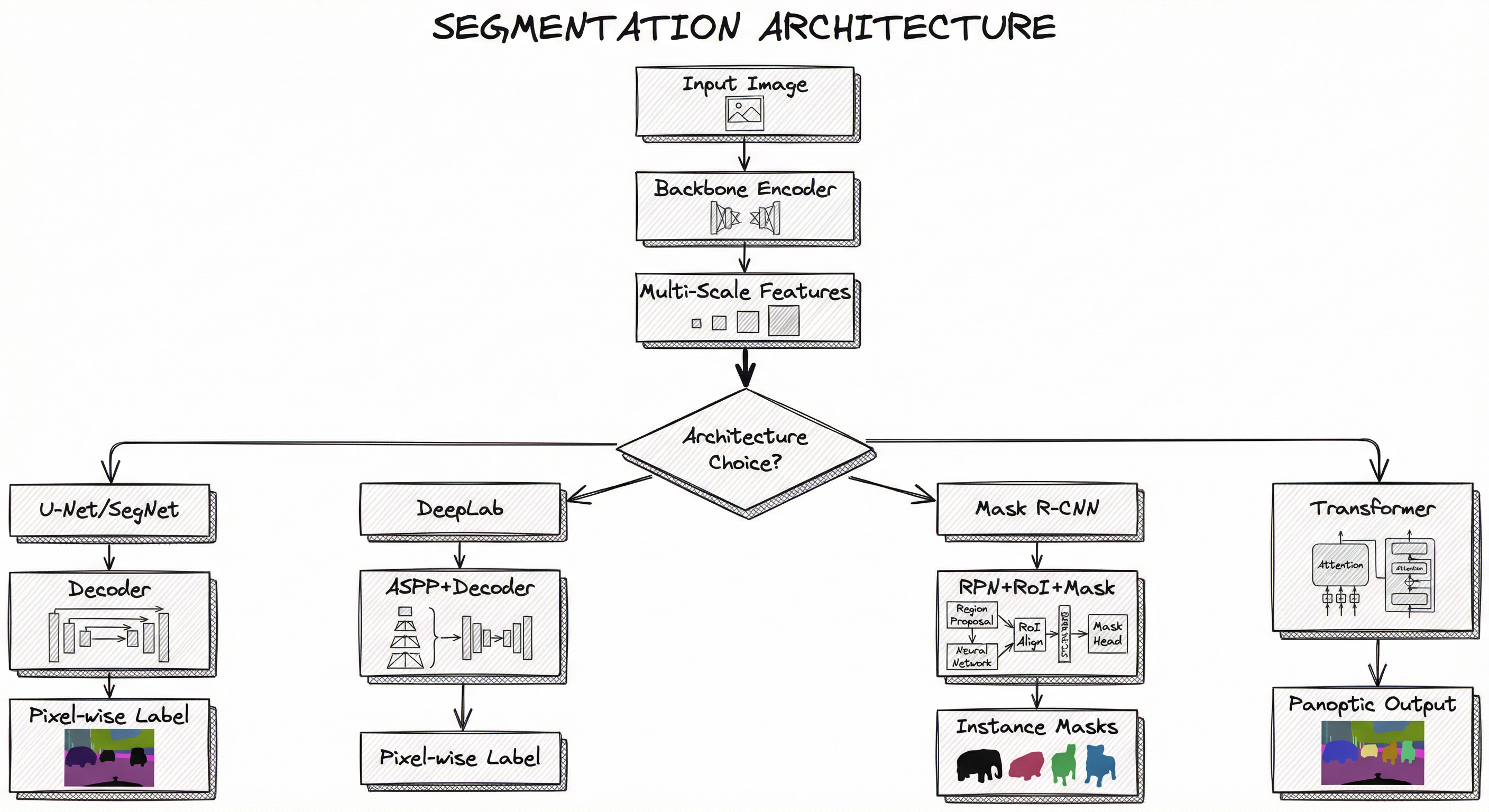
A flowchart showing an input image feeding into a backbone encoder, which produces multi-scale features. These features then branch into four architectural paths: (1) U-Net/SegNet path with decoder and skip connections producing pixel-wise labels, (2) DeepLab path with ASPP and decoder producing pixel-wise labels, (3) Mask R-CNN path with RPN, RoI Align, and mask head producing instance masks, and (4) Transformer path with masked attention and query decoder producing unified panoptic output.
How to Implement
Choosing Your Approach
Implementation strategy depends heavily on which segmentation paradigm you need and your deployment constraints:
For semantic segmentation: Start with DeepLab v3+ or a U-Net variant. These are well-understood, have excellent library support, and train efficiently. If you are working in medical imaging, U-Net (or its self-configuring variant nnU-Net) is the de facto standard -- it has won more medical segmentation challenges than any other architecture.
For instance segmentation: Mask R-CNN remains the production workhorse. It is thoroughly battle-tested, well-supported in Detectron2, and offers a clean separation between detection and mask prediction. For real-time needs, YOLO-based segmentation models (YOLOv8-seg, YOLOv11-seg) offer 30+ FPS on modern GPUs with competitive accuracy.
For panoptic segmentation: Mask2Former or OneFormer are the state of the art. OneFormer is particularly attractive because a single model handles all three tasks, reducing deployment complexity.
For zero-shot / promptable segmentation: Meta's Segment Anything Model (SAM / SAM 2) is the breakthrough option. You provide a point, box, or text prompt, and SAM produces a high-quality mask for any object -- no task-specific training required. SAM 2 extends this to video.
Cost Note: Training a DeepLab v3+ model on Cityscapes from a pretrained backbone takes approximately 8-12 hours on a single A100 GPU (~INR 250-500/hour on Indian cloud providers like E2E Networks, or 100-180) for a small dataset. For inference, a T4 GPU (~INR 25-35/hour, $0.30-0.40/hour) handles most segmentation models at production-viable throughput.
Data Annotation
Segmentation requires the most expensive annotation among vision tasks. Per-image annotation times:
- Bounding boxes: 30-60 seconds per image
- Semantic segmentation masks: 5-15 minutes per image
- Instance segmentation masks: 10-30 minutes per image
- Panoptic segmentation: 20-45 minutes per image
In India, annotation costs range from INR 15-50 (900-3,000) for annotations alone. This is why techniques like semi-supervised learning, pseudo-labeling with SAM, and active learning are increasingly important.
import torch
import torchvision.transforms as T
from torchvision.models.segmentation import deeplabv3_resnet101
from PIL import Image
import numpy as np

# Load pretrained DeepLab v3+ (trained on COCO + VOC)
model = deeplabv3_resnet101(pretrained=True)
model.eval()

# Preprocessing pipeline
preprocess = T.Compose([
    T.Resize(520),
    T.ToTensor(),
    T.Normalize(mean=[0.485, 0.456, 0.406], std=[0.229, 0.224, 0.225]),
])

# Load and preprocess image
image = Image.open("street_scene.jpg").convert("RGB")
input_tensor = preprocess(image).unsqueeze(0)  # Add batch dim

# Inference
with torch.no_grad():
    output = model(input_tensor)["out"]  # Shape: (1, 21, H, W)
    predictions = output.argmax(dim=1).squeeze().numpy()  # (H, W)

# predictions is now a 2D array where each value is a class ID (0-20)
# 0=background, 1=aeroplane, 7=car, 15=person, etc.
print(f"Unique classes found: {np.unique(predictions)}")
print(f"Segmentation map shape: {predictions.shape}")
This example loads a pretrained DeepLab v3+ model from torchvision and runs inference on a single image. The model outputs 21-class logits (PASCAL VOC classes) at each pixel position. The argmax operation converts logits to a label map. For production use, you would replace the pretrained model with one fine-tuned on your domain-specific dataset. Note that torchvision's deeplabv3_resnet101 uses a ResNet-101 backbone with atrous convolutions and ASPP.
from detectron2.engine import DefaultPredictor
from detectron2.config import get_cfg
from detectron2 import model_zoo
from detectron2.utils.visualizer import Visualizer
from detectron2.data import MetadataCatalog
import cv2

# Configure Mask R-CNN with ResNet-50 FPN backbone
cfg = get_cfg()
cfg.merge_from_file(
    model_zoo.get_config_file("COCO-InstanceSegmentation/mask_rcnn_R_50_FPN_3x.yaml")
)
cfg.MODEL.WEIGHTS = model_zoo.get_checkpoint_url(
    "COCO-InstanceSegmentation/mask_rcnn_R_50_FPN_3x.yaml"
)
cfg.MODEL.ROI_HEADS.SCORE_THRESH_TEST = 0.5  # confidence threshold
cfg.MODEL.DEVICE = "cuda"  # or "cpu"

predictor = DefaultPredictor(cfg)

# Run inference
image = cv2.imread("street_scene.jpg")
outputs = predictor(image)

# Extract results
instances = outputs["instances"].to("cpu")
print(f"Detected {len(instances)} instances")
print(f"Classes: {instances.pred_classes.numpy()}")    # class IDs
print(f"Scores: {instances.scores.numpy()}")            # confidence scores
print(f"Masks shape: {instances.pred_masks.shape}")      # (N, H, W) binary masks
print(f"Boxes: {instances.pred_boxes.tensor.numpy()}")   # bounding boxes

# Visualize
v = Visualizer(image[:, :, ::-1], MetadataCatalog.get(cfg.DATASETS.TRAIN[0]))
out = v.draw_instance_predictions(instances)
cv2.imwrite("output_segmentation.jpg", out.get_image()[:, :, ::-1])
Detectron2 (by Meta) is the go-to library for instance and panoptic segmentation. This example loads a pretrained Mask R-CNN with a ResNet-50 FPN backbone trained on COCO (80 classes). The output includes per-instance binary masks, class predictions, confidence scores, and bounding boxes. For custom datasets, you would register your dataset with Detectron2 and fine-tune using their training loop. The SCORE_THRESH_TEST parameter is critical -- set it too low and you get false positives, too high and you miss objects.
from segment_anything import sam_model_registry, SamPredictor
import cv2
import numpy as np

# Load SAM model (ViT-H for best quality, ViT-B for speed)
sam = sam_model_registry["vit_h"](checkpoint="sam_vit_h_4b8939.pth")
sam.to(device="cuda")
predictor = SamPredictor(sam)

# Load image and set it
image = cv2.imread("medical_scan.jpg")
image_rgb = cv2.cvtColor(image, cv2.COLOR_BGR2RGB)
predictor.set_image(image_rgb)  # Encodes image (run once per image)

# Prompt with a point (x, y) -- e.g., click on a tumor
input_point = np.array([[256, 256]])  # (x, y) coordinates
input_label = np.array([1])           # 1 = foreground, 0 = background

masks, scores, logits = predictor.predict(
    point_coords=input_point,
    point_labels=input_label,
    multimask_output=True,  # Returns 3 masks at different granularities
)

# masks: (3, H, W) boolean arrays -- pick the highest-scoring one
best_mask = masks[np.argmax(scores)]
print(f"Best mask score: {scores.max():.3f}")
print(f"Mask area: {best_mask.sum()} pixels ({best_mask.mean()*100:.1f}% of image)")

# Prompt with a bounding box
input_box = np.array([100, 100, 400, 400])  # [x1, y1, x2, y2]
masks_box, scores_box, _ = predictor.predict(
    box=input_box,
    multimask_output=False,
)
print(f"Box-prompted mask score: {scores_box[0]:.3f}")
SAM (Segment Anything Model) is a foundation model that can segment any object given a prompt -- a point, a bounding box, or a text description. This is revolutionary because you do not need to train a task-specific model. The set_image call runs the heavy image encoder once (~0.5s on GPU), and subsequent predict calls with different prompts are fast (~50ms). The multimask_output=True option returns three masks at different granularities (sub-part, part, whole object), which is useful when the prompt is ambiguous. SAM is particularly powerful for interactive annotation tools and bootstrapping training data for specialized models.
import torch
import torch.nn as nn
import segmentation_models_pytorch as smp
from torch.utils.data import DataLoader

# Build U-Net with pretrained EfficientNet-B4 encoder
model = smp.Unet(
    encoder_name="efficientnet-b4",
    encoder_weights="imagenet",
    in_channels=3,
    classes=1,  # Binary segmentation (e.g., tumor vs background)
    activation=None,  # Raw logits; apply sigmoid in loss
)

# Combined loss: BCE + Dice (best practice for medical segmentation)
criterion = smp.losses.DiceLoss(mode="binary") + smp.losses.SoftBCEWithLogitsLoss()

optimizer = torch.optim.AdamW(model.parameters(), lr=1e-4, weight_decay=1e-4)
scheduler = torch.optim.lr_scheduler.CosineAnnealingLR(optimizer, T_max=50)

# Training loop (simplified)
model.train()
for epoch in range(50):
    epoch_loss = 0
    for images, masks in train_loader:  # images: (B,3,H,W), masks: (B,1,H,W)
        images, masks = images.cuda(), masks.cuda()
        predictions = model(images)
        loss = criterion(predictions, masks)

        optimizer.zero_grad()
        loss.backward()
        optimizer.step()
        epoch_loss += loss.item()

    scheduler.step()
    avg_loss = epoch_loss / len(train_loader)
    print(f"Epoch {epoch+1}/50 | Loss: {avg_loss:.4f}")

# Evaluation
model.eval()
with torch.no_grad():
    for images, masks in val_loader:
        preds = torch.sigmoid(model(images.cuda())) > 0.5
        iou = (preds & masks.cuda().bool()).sum() / (preds | masks.cuda().bool()).sum()
        print(f"Validation IoU: {iou.item():.4f}")
This example uses the excellent segmentation_models_pytorch library to build a U-Net with a pretrained EfficientNet-B4 encoder. The combined Dice + BCE loss is the standard practice for medical segmentation -- Dice loss handles class imbalance well (tumors are often tiny relative to the background), while BCE provides stable per-pixel gradients. The CosineAnnealing scheduler is preferred over StepLR for segmentation training. Note the binary threshold of 0.5 during evaluation -- in production, you would tune this threshold on the validation set.
# Example training config for DeepLab v3+ on Cityscapes (MMSegmentation format)
_base_ = [
    '../_base_/models/deeplabv3plus_r101-d8.py',
    '../_base_/datasets/cityscapes.py',
    '../_base_/default_runtime.py',
    '../_base_/schedules/schedule_80k.py'
]
model:
  backbone:
    type: ResNet
    depth: 101
    dilations: [1, 1, 2, 4]
    strides: [1, 2, 1, 1]
    norm_cfg:
      type: SyncBN
  decode_head:
    type: DepthwiseSeparableASPPHead
    dilations: [1, 6, 12, 18]
    c1_in_channels: 256
    c1_channels: 48
    num_classes: 19
    loss_decode:
      type: CrossEntropyLoss
      use_sigmoid: false
      class_weight: null  # Use uniform weights; tune per-class for imbalanced data
data:
  samples_per_gpu: 4
  workers_per_gpu: 4
  train:
    type: CityscapesDataset
    data_root: data/cityscapes/
    img_dir: leftImg8bit/train
    ann_dir: gtFine/train
    pipeline:
      - type: Resize
        img_scale: [2048, 1024]
      - type: RandomCrop
        crop_size: [512, 1024]
      - type: RandomFlip
        prob: 0.5
      - type: PhotoMetricDistortion
      - type: Normalize
optimizer:
  type: SGD
  lr: 0.01
  momentum: 0.9
  weight_decay: 0.0005
lr_config:
  policy: poly
  power: 0.9
  min_lr: 0.0001
Common Implementation Mistakes
- ●
Ignoring class imbalance: In most segmentation datasets, background dominates (often 60-80% of pixels). Using unweighted cross-entropy causes the model to predict background everywhere and still achieve 70%+ accuracy. Always use class-weighted loss, focal loss, or Dice loss. This is especially acute in medical imaging where a tumor might occupy 2% of the image.
- ●
Wrong input resolution: Segmentation models are sensitive to input resolution. Training at 512x512 but deploying at 1920x1080 causes severe quality degradation. Always match training and inference resolutions, or use multi-scale inference with result fusion.
- ●
Neglecting boundary quality: Standard IoU/Dice metrics weight all pixels equally, but boundary pixels are what matter most for downstream tasks. Add boundary-focused losses (e.g., boundary loss, Hausdorff distance loss) and evaluate with boundary-specific metrics for critical applications.
- ●
Using the wrong segmentation paradigm: Choosing semantic segmentation when you actually need instance-level distinctions (e.g., counting individual cells in microscopy) leads to merged predictions for touching objects. Think carefully about whether you need class-level or instance-level output.
- ●
Skipping test-time augmentation (TTA): For critical applications, TTA (running inference on flipped and multi-scale versions of the image, then averaging predictions) can improve mIoU by 1-3% at the cost of 4-8x inference time. Many teams skip this and leave accuracy on the table.
- ●
Not handling edge cases in post-processing: Raw model output often contains small spurious predictions and holes. Connected component analysis, morphological operations (opening/closing), and minimum-area thresholds are essential post-processing steps that teams frequently forget.
When Should You Use This?
Use When
You need pixel-precise boundaries of objects or regions -- bounding boxes are too coarse for your downstream task (path planning, measurement, interaction)
Your application involves medical imaging where precise delineation of anatomical structures, lesions, or tumors directly affects diagnosis and treatment planning
You are building autonomous driving perception where understanding the exact extent of drivable area, lane markings, pedestrians, and obstacles is safety-critical
You need to count or track individual instances of overlapping objects (cells in microscopy, products on a conveyor belt, people in a crowd)
Your use case involves image editing or compositing -- background removal, product photography, video effects, or augmented reality overlays
You are performing remote sensing or satellite image analysis for land-use mapping, crop monitoring, urban planning, or disaster assessment
You need quality inspection in manufacturing where defect localization at the pixel level determines accept/reject decisions
Avoid When
Simple classification suffices: If you only need to know whether an image contains a cat or a dog, classification is orders of magnitude cheaper to train and deploy than segmentation
Bounding boxes are good enough: If pixel-level boundaries add no value to your downstream task (e.g., inventory counting from surveillance), object detection is simpler and faster
Your annotation budget is limited: Segmentation masks cost 10-50x more to annotate than bounding boxes. If you cannot afford the annotation investment, consider detection with SAM-based pseudo-labeling as a bridge
Real-time requirements on edge devices without GPU: Even lightweight segmentation models require significant compute. On CPU-only embedded devices, simpler approaches (thresholding, classical CV) may be necessary
The scene is too simple: For binary foreground/background separation with high contrast (e.g., dark objects on a white conveyor belt), classical computer vision (Otsu thresholding, watershed) is faster and cheaper than deep learning
Key Tradeoffs
Accuracy vs. Speed
The fundamental tradeoff in segmentation is between prediction quality and inference latency. Here is a representative comparison on Cityscapes validation:
| Model | mIoU (%) | Params (M) | FPS (A100) | FPS (T4) |
|---|---|---|---|---|
| DeepLab v3+ (ResNet-101) | 80.9 | 62.7 | 28 | 8 |
| Mask2Former (Swin-L) | 83.3 | 216 | 12 | 3 |
| BiSeNet v2 (real-time) | 72.6 | 3.4 | 156 | 65 |
| YOLOv8-seg (Large) | 76.2 | 52.2 | 85 | 25 |
| SAM (ViT-H) | N/A* | 636 | 4 | <1 |
*SAM is zero-shot and not directly comparable on fixed benchmarks, but its mask quality is excellent when given good prompts.
For autonomous driving, you typically need 20+ FPS at 1080p, which narrows the field to lightweight models (BiSeNet, DDRNet, PIDNet) or well-optimized standard models with TensorRT. For medical imaging, offline processing at 1-5 FPS is usually acceptable, so you can afford heavier models.
Generalization vs. Specialization
Foundation models like SAM generalize across domains but may not match the accuracy of a domain-specific model fine-tuned on your exact data distribution. For example, SAM achieves ~85% IoU on generic objects but a fine-tuned nnU-Net achieves ~92% Dice on liver tumor segmentation. The question is whether the 7% accuracy gap justifies the cost of collecting and annotating domain-specific data.
Memory and Compute Budget
Segmentation models are memory-hungry because they operate on full-resolution feature maps. A Mask2Former with Swin-L backbone requires ~12 GB VRAM for inference at 1024x1024. On cloud infrastructure, this means you need at least a T4 (16 GB) or better. On Indian cloud providers like E2E Networks, a T4 instance costs ~INR 25-35/hour (2.50-5.00/hour).
Rule of Thumb: For production deployment, optimize for the cheapest GPU that meets your latency SLA. Most segmentation workloads fit comfortably on a T4 after TensorRT optimization.
Alternatives & Comparisons
Object detection provides rectangular bounding boxes around objects -- faster to train, cheaper to annotate, and lower inference cost. Choose detection when pixel-level precision is unnecessary and bounding boxes provide sufficient localization. Choose segmentation when you need exact shapes, contours, or area measurements (e.g., tumor volume, road surface area, precise occlusion handling).
Classification assigns a single label to the entire image, with no spatial information. It is the simplest and cheapest vision task. Choose classification for binary decisions (defective/non-defective, disease/healthy) where localization is not needed. Choose segmentation when you need to know where and what shape the relevant regions are.
Image preprocessing (resizing, normalization, augmentation) is an upstream step that feeds into segmentation, not an alternative to it. However, classical preprocessing techniques like thresholding, edge detection, and watershed can sometimes achieve adequate segmentation for simple scenes (high-contrast, controlled lighting) without deep learning. Choose classical preprocessing when the visual problem is simple and deep learning is overkill.
Pros, Cons & Tradeoffs
Advantages
Pixel-level precision enables downstream tasks that bounding boxes cannot support: volumetric measurement, precise occlusion reasoning, and contour-based shape analysis. A segmentation mask tells you not just where an object is, but its exact extent.
Rich scene understanding -- panoptic segmentation provides a complete parsing of the scene where every pixel is accounted for, enabling applications like autonomous driving planning, robotic manipulation, and augmented reality.
Foundation models (SAM) democratize access -- zero-shot segmentation means you can segment novel object categories without collecting or annotating training data, drastically reducing the time-to-deployment for new use cases.
Transfer learning is highly effective -- pretrained encoders (ImageNet, COCO) transfer well to domain-specific segmentation tasks. Fine-tuning on even 100-500 annotated images often yields production-viable models for specialized domains like medical imaging or industrial inspection.
Mature ecosystem of tools and frameworks -- Detectron2, MMSegmentation, segmentation_models_pytorch, Ultralytics YOLO, and Hugging Face Transformers all provide production-ready implementations with pretrained weights.
Directly optimizable metrics -- Dice loss and IoU-based losses allow you to train models that directly optimize the evaluation metrics, unlike classification where surrogate losses dominate.
Disadvantages
Annotation cost is prohibitive -- pixel-level masks cost 10-50x more per image than bounding boxes. A 5,000-image medical dataset can cost INR 2-3 lakh ($2,500-3,600) to annotate, and larger datasets scale linearly.
High compute requirements -- segmentation models process full-resolution feature maps, demanding 2-4x more VRAM and FLOPs than equivalent classification or detection models. Training DeepLab v3+ on Cityscapes requires 8-12 A100-hours.
Inference latency is significant -- even optimized models like BiSeNet v2 run at 65 FPS on a T4, which may not meet real-time requirements for high-resolution video (4K at 30 FPS). Edge deployment remains challenging for complex models.
Boundary quality is hard to perfect -- segmentation models struggle with thin structures (bicycle spokes, hair, power lines), fine boundaries between similar classes, and heavily occluded objects. Post-processing helps but does not fully solve the problem.
Domain shift sensitivity -- models trained on daytime urban scenes (Cityscapes) degrade significantly on nighttime, rainy, or rural scenes. Indian road conditions (unstructured traffic, diverse vehicles, unpainted road boundaries) are particularly challenging for models trained on Western datasets.
Evaluation metrics can be misleading -- high mIoU can mask poor performance on rare classes. A model with 78% mIoU on Cityscapes might have only 40% IoU on the 'bicycle' class, which could be safety-critical.
Failure Modes & Debugging
Class Imbalance Collapse
Cause
The model learns to predict the majority class (typically background) for all pixels because unweighted cross-entropy loss rewards this trivially correct prediction. This is especially common in medical imaging where the target structure (tumor, lesion) occupies <5% of the image.
Symptoms
Training loss decreases but IoU/Dice for minority classes remains near zero. The model produces nearly all-background predictions. Pixel accuracy looks high (90%+) but is meaningless.
Mitigation
Use Dice loss or focal loss instead of (or in addition to) standard cross-entropy. Apply per-class weights inversely proportional to class frequency. Oversample patches containing minority classes. Monitor per-class IoU, not just mean IoU, during training.
Boundary Bleeding / Fuzzy Edges
Cause
Aggressive downsampling in the encoder loses fine spatial information, and the decoder cannot fully recover it. Skip connections help but are insufficient when encoder resolution drops below 1/32 of the original. Also occurs when training resolution is too low.
Symptoms
Predicted masks have blurry, imprecise boundaries that leak into adjacent regions. Two objects of the same class get merged when they are close together. Small objects disappear entirely.
Mitigation
Use architectures with higher-resolution feature maps (DeepLab with dilated convolutions instead of pooling). Add boundary loss terms. Increase training resolution. Use CRF-based post-processing (though this adds latency). Employ multi-scale inference.
Domain Shift Degradation
Cause
Model trained on one visual domain (e.g., clear-weather European streets from Cityscapes) is deployed in a different domain (e.g., dusty Indian roads with chaotic traffic, monsoon conditions, or nighttime scenes). The feature distributions differ substantially.
Symptoms
mIoU drops 10-30% when moving to the target domain. Specific classes that differ between domains (auto-rickshaws, unpainted road boundaries, mixed pedestrian-vehicle traffic) are consistently misclassified.
Mitigation
Fine-tune on target domain data -- even 200-500 annotated images from the deployment environment can recover most of the performance. Use domain adaptation techniques (adversarial training, style transfer). Leverage the Indian Driving Dataset (IDD) from IIIT Hyderabad for Indian road scenes.
Small Object Disappearance
Cause
Objects that are small relative to the image (traffic signs at distance, small tumors, thin structures like poles and wires) get lost during encoder downsampling. By the time features reach 1/32 resolution, a 16-pixel object is less than one feature cell.
Symptoms
Small objects are consistently absent from predictions. Recall for small objects is dramatically lower than for large objects. mIoU looks acceptable overall but hides severe failure on small-object classes.
Mitigation
Use Feature Pyramid Networks to detect at multiple scales. Train with higher input resolution. Use tile-based inference where the image is split into overlapping patches. Apply class-specific evaluation and set minimum performance thresholds for safety-critical small-object classes.
Instance Merging in Crowded Scenes
Cause
In instance segmentation, closely packed objects of the same class (a crowd of people, clustered cells, products on a shelf) get merged into a single instance because the model cannot find clear boundaries between overlapping instances.
Symptoms
Instance count is consistently lower than ground truth. Merged masks have irregular, non-convex shapes. AP (Average Precision) is significantly lower at high IoU thresholds (AP75 vs AP50).
Mitigation
Use architectures with strong instance separation capabilities (PointRend, Mask R-CNN with finer-grained RoI features). Apply non-maximum suppression with tuned thresholds. Post-process with watershed or morphological separation. Consider panoptic architectures that explicitly model instance boundaries.
Memory Overflow During Training
Cause
Segmentation models maintain full-resolution feature maps through the network, consuming 2-4x more VRAM than classification. Training on high-resolution images (e.g., 2048x1024 Cityscapes) with a large batch size easily exceeds GPU memory.
Symptoms
CUDA out-of-memory errors. Training crashes on the first forward pass. Silently degraded performance when the framework falls back to gradient checkpointing without informing the user.
Mitigation
Use mixed-precision training (FP16) to halve memory usage. Reduce batch size and compensate with gradient accumulation. Use random cropping during training (standard practice -- train on 512x512 crops even if full images are 2048x1024). Enable gradient checkpointing explicitly.
Placement in an ML System
Where Segmentation Fits in the ML Pipeline
In an autonomous driving stack, segmentation sits in the perception layer, immediately after image preprocessing (debayering, lens distortion correction, exposure normalization) and alongside or after object detection. The segmentation output -- a per-pixel semantic map plus instance masks for dynamic objects -- feeds into the planning module, which uses it to identify drivable area, lane boundaries, and obstacle contours.
In a medical imaging pipeline, segmentation is typically the core inference step. Raw DICOM images are preprocessed (windowing, normalization, resampling to isotropic resolution), then passed through a segmentation model (usually U-Net or nnU-Net). The output masks feed into measurement extraction (tumor volume, organ dimensions), treatment planning (radiation beam targeting), and longitudinal tracking (change detection across scans).
In an e-commerce image pipeline (think Flipkart, Myntra, or Amazon product photography), segmentation performs background removal and product isolation. The input is a raw product photo; the output is an RGBA image with the product precisely masked. This feeds into downstream systems for catalog standardization, virtual try-on, and augmented reality product placement.
Key Insight: Segmentation is almost never a standalone system. It is a perception primitive that feeds spatial understanding into domain-specific decision-making. The value of segmentation is measured not by mIoU alone but by how accurately it enables the downstream task.
Pipeline Stage
Inference / Perception
Upstream
- image-preprocessor
- image-classifier
Downstream
- object-detector
Scaling Bottlenecks
Inference latency: Segmentation is the most compute-intensive per-pixel prediction task. At 1080p resolution, a DeepLab v3+ model produces 2 million pixel predictions per frame. For real-time video (30 FPS), that is 60 million pixel classifications per second. Even on an A100, this limits model complexity.
Memory bandwidth: Feature maps at 1/4 resolution for a 1080p image are 270x480x256 = ~140 MB in FP32. Moving this through the decoder requires substantial memory bandwidth, making segmentation more memory-bound than compute-bound on modern GPUs.
Annotation throughput: Scaling training data is bottlenecked by annotation speed. A trained annotator can produce 4-8 semantic segmentation masks per hour, versus 60-120 bounding boxes per hour. This 10-15x annotation cost difference limits dataset scale.
Multi-GPU training: Segmentation benefits from synchronized batch normalization (SyncBN) across GPUs because the effective batch size per GPU is small (due to high memory usage). This requires all-reduce communication at every BN layer, adding 10-20% training overhead.
Some concrete numbers: serving a DeepLab v3+ model at 1080p resolution, a single T4 handles ~8 requests/second. For a video analytics platform processing 100 camera streams at 5 FPS, you need ~63 T4 GPUs, costing approximately INR 50,000-70,000/day ($600-850/day) on cloud infrastructure.
Production Case Studies
Waymo's perception system uses multi-task neural networks that perform semantic segmentation alongside object detection and depth estimation from camera and LiDAR inputs. Their perception pipeline fuses segmentation outputs across multiple sensor modalities to build a coherent 3D scene understanding. Segmentation specifically identifies drivable surface, lane markings, curbs, and vegetation to inform the planning module.
Over 20 million autonomous miles driven safely, with the perception system processing sensor data at real-time speeds across a fleet of vehicles operating in multiple US cities.
AIIMS New Delhi, in collaboration with the Centre for Development of Advanced Computing (CDAC) Pune, launched iOncology.ai -- a deep learning platform that uses segmentation models to analyze radiological and histopathological images for early detection and treatment planning of breast and ovarian cancers. The system segments tumor regions from medical scans to provide precise volumetric measurements that guide treatment decisions.
The platform was trained on approximately 500,000 images from 1,500 patient cases and is being validated across five district hospitals in India, demonstrating the potential for AI-powered segmentation to improve cancer care in resource-constrained settings.
Tesla's Full Self-Driving (FSD) system uses a HydraNet architecture where a single shared backbone feeds into multiple task-specific heads, including semantic segmentation for drivable area, lane line detection, and freespace estimation. The system processes 8 camera feeds simultaneously and produces dense per-pixel predictions for road structure understanding. Their segmentation models are trained on data from millions of fleet vehicles.
3 billion+ FSD miles driven by customers as of January 2025, with the perception system (including segmentation) running on custom Tesla HW3/HW4 chips at real-time speeds. Tesla invested $10 billion cumulatively in AI training compute by end of 2024.
The Indian Driving Dataset (IDD), developed by IIIT Hyderabad in collaboration with Intel, provides 10,000 finely annotated images with 34 segmentation classes collected from driving sequences in Hyderabad and Bangalore. Unlike Western datasets like Cityscapes, IDD captures unstructured Indian road conditions -- mixed traffic with auto-rickshaws, two-wheelers, pedestrians, animals, and unpainted road boundaries -- making it essential for training segmentation models that work on Indian roads.
IDD has become the standard benchmark for autonomous driving perception in Indian conditions. It has spawned a family of datasets (IDD-3D, IDD-AW for adverse weather) and is used by research groups worldwide studying perception in unstructured driving environments.
Cloudflare built an image background removal service using segmentation models (evaluating U2-Net and IS-Net) deployed on their global edge network. The system performs semantic segmentation to separate foreground objects from backgrounds, producing alpha mattes for product photography, profile pictures, and content creation. They evaluated multiple segmentation architectures for the tradeoff between mask quality and inference speed on their Workers AI platform.
Successfully deployed as a production API serving millions of background removal requests, demonstrating that segmentation models can be deployed at edge-scale with sub-second latency per image.
Tooling & Ecosystem
Meta's next-generation library for object detection and segmentation. Provides production-ready implementations of Mask R-CNN, Panoptic FPN, PointRend, and Mask2Former. Includes a model zoo with pretrained weights on COCO and other datasets. The de facto standard for instance and panoptic segmentation research and production.
OpenMMLab's comprehensive semantic segmentation toolbox. Supports 40+ architectures (DeepLab, PSPNet, U-Net, SegFormer, Mask2Former) with unified training and evaluation pipelines. Excellent for benchmarking and rapid prototyping. Part of the broader OpenMMLab ecosystem.
Meta's foundation model for promptable segmentation. Trained on 11M images with 1.1B masks. Supports point, box, and mask prompts for zero-shot segmentation of any object. SAM 2 extends to video segmentation. Revolutionary for annotation bootstrapping and interactive segmentation tools.
High-level library providing 9 segmentation architectures (U-Net, FPN, DeepLabV3+, LinkNet, PSPNet, etc.) with 500+ pretrained encoders. The simplest way to build a custom segmentation model in PyTorch. Widely used in medical imaging and Kaggle competitions.
YOLO-based instance segmentation models offering real-time inference (30-85 FPS on A100). YOLOv8-seg and YOLO11-seg provide competitive accuracy with significantly lower latency than Mask R-CNN. Excellent for edge deployment and video processing applications.
A self-configuring framework that automatically adapts U-Net architecture, preprocessing, training, and post-processing for any new medical segmentation task. Has won more medical segmentation challenges than any other method. The gold standard for medical imaging segmentation.
Hosts pretrained segmentation models (SegFormer, Mask2Former, OneFormer, SAM) with unified inference APIs. Includes model cards, benchmarks, and demo spaces. The easiest way to try state-of-the-art segmentation models without writing training code.
Research & References
Long, Shelhamer & Darrell (2015)CVPR 2015
The foundational paper that introduced fully convolutional networks (FCNs) for dense prediction, replacing fully connected layers with convolutional layers to produce spatial output. Established the encoder-decoder paradigm that dominates segmentation to this day.
Ronneberger, Fischer & Brox (2015)MICCAI 2015
Introduced the U-Net architecture with symmetric encoder-decoder and skip connections. Demonstrated that segmentation models can be trained effectively with very few annotated images. Became the de facto standard for medical image segmentation.
He, Gkioxari, Dollar & Girshick (2017)ICCV 2017
Extended Faster R-CNN with a parallel mask prediction branch for instance segmentation. Introduced RoI Align for precise spatial feature extraction. Set the standard for two-stage instance segmentation that remains dominant in production systems.
Chen, Zhu, Papandreou, Schroff & Adam (2018)ECCV 2018
Combined atrous spatial pyramid pooling (ASPP) with an encoder-decoder structure and depthwise separable convolutions. Achieved 89.0% mIoU on PASCAL VOC 2012 and 82.1% on Cityscapes, establishing the DeepLab series as the leading semantic segmentation approach.
Kirillov, He, Girshick & Dollar (2019)CVPR 2019
Proposed the panoptic segmentation task that unifies semantic and instance segmentation, requiring every pixel to receive both a class label and an instance ID. Introduced the Panoptic Quality (PQ) metric that decomposes into recognition and segmentation quality.
Kirillov, Mintun, Ravi et al. (2023)ICCV 2023
Introduced the Segment Anything Model (SAM), a foundation model trained on 11M images and 1.1B masks. SAM can segment any object given a point, box, or text prompt with zero-shot generalization. Fundamentally changed the segmentation landscape by making high-quality segmentation accessible without task-specific training.
Ravi, Gabeur, Hu et al. (2024)arXiv preprint (Meta AI)
Extended SAM to video segmentation with a streaming memory architecture that tracks and segments objects across frames in near real-time. Trained on SA-V, a new dataset of 50.9K videos with 642.6K masklets.
Cheng, Misra, Schwing, Kirillov & Girdhar (2022)CVPR 2022
Proposed a transformer-based architecture that handles semantic, instance, and panoptic segmentation with the same model architecture, using masked cross-attention and learnable queries. Achieved state-of-the-art results across all three tasks.
Jain, Li, Chiu, Hassani, Orlov & Shi (2023)CVPR 2023
Introduced a task-conditioned joint training strategy that trains a single model on all three segmentation tasks simultaneously. A single OneFormer model outperforms specialized Mask2Former models trained separately on each task, achieving 68.5 PQ on Cityscapes.
Isensee, Jaeger, Kohl, Petersen & Maier-Hein (2021)Nature Methods, Vol. 18
Presented a self-adapting framework that automatically configures U-Net architecture, preprocessing, and training for any medical segmentation task. Without manual intervention, nnU-Net surpassed most specialized solutions on 23 public biomedical segmentation benchmarks.
Interview & Evaluation Perspective
Common Interview Questions
- ●
What is the difference between semantic, instance, and panoptic segmentation? When would you choose each?
- ●
How does U-Net work, and why are skip connections important for segmentation?
- ●
Explain the Mask R-CNN architecture. What role does RoI Align play?
- ●
How would you handle severe class imbalance in a medical image segmentation task?
- ●
What is IoU and how does it differ from Dice coefficient? When would you prefer one over the other?
- ●
How would you deploy a segmentation model for real-time autonomous driving at 30 FPS?
- ●
How does Segment Anything (SAM) differ from traditional segmentation approaches? What are its limitations?
- ●
Design a segmentation pipeline for quality inspection in a manufacturing plant processing 1000 items/hour.
Key Points to Mention
- ●
The three segmentation paradigms serve different needs: semantic for scene parsing, instance for counting and tracking, panoptic for complete scene understanding. Choosing the wrong paradigm wastes resources or misses requirements.
- ●
Class imbalance is the #1 practical challenge. Always use Dice loss or focal loss, not raw cross-entropy. Monitor per-class IoU, not just mIoU, because aggregate metrics hide failures on rare but important classes.
- ●
Encoder-decoder architecture with skip connections is the fundamental building block. The encoder captures what (semantics), the decoder recovers where (spatial detail), and skip connections prevent information loss during the bottleneck.
- ●
For production deployment, model optimization is essential: TensorRT, ONNX Runtime, or TorchScript can improve inference speed by 2-5x. Mixed-precision (FP16) halves memory with <1% accuracy loss.
- ●
SAM changed the game for annotation and prototyping but is not a replacement for fine-tuned models in specialized domains. Domain-specific models still outperform SAM by 5-10% IoU when trained on sufficient data.
- ●
Indian road conditions present unique challenges for autonomous driving segmentation: unstructured traffic, diverse vehicle types (auto-rickshaws, handcarts, bullock carts), unpainted road boundaries, and extreme weather. The IDD dataset specifically addresses these challenges.
Pitfalls to Avoid
- ●
Confusing semantic and instance segmentation -- saying 'I would use U-Net for counting objects' (U-Net produces semantic masks that merge instances of the same class; you need instance segmentation for counting).
- ●
Claiming high mIoU means the model works well -- without checking per-class performance. A model with 80% mIoU might have 20% IoU on the class that matters most for your application.
- ●
Ignoring inference cost -- proposing a Mask2Former with Swin-L backbone for a real-time edge deployment that has 50ms latency budget. Always ground architectural choices in compute constraints.
- ●
Forgetting post-processing -- raw model output almost always needs morphological cleanup, connected component filtering, and minimum area thresholds before it is production-ready.
Senior-Level Expectation
A senior candidate should discuss the full system design: data collection strategy (active learning, SAM-bootstrapped annotation, synthetic data generation), annotation pipeline and quality control, model selection with quantitative justification tied to deployment constraints (latency, memory, accuracy requirements), training infrastructure (distributed training with SyncBN, mixed precision, gradient checkpointing), evaluation methodology (per-class metrics, boundary metrics, calibration analysis), deployment optimization (TensorRT, quantization, model distillation), monitoring in production (drift detection on input distribution, prediction confidence monitoring, periodic human audit), and cost analysis (training compute, inference infrastructure, annotation budget). The ability to reason about the cost-quality Pareto frontier -- especially relevant for Indian startups operating under tight budgets -- is what separates senior from mid-level engineers.
Summary
Image segmentation is the task of assigning a class label -- and optionally a unique instance identity -- to every pixel in an image, producing the most spatially precise form of visual understanding available. The three paradigms -- semantic, instance, and panoptic segmentation -- serve progressively more demanding requirements, from scene-level parsing to individual object identification to complete scene decomposition.
The architectural evolution from FCN (2015) through U-Net and Mask R-CNN to modern transformer-based models like Mask2Former, OneFormer, and the Segment Anything Model (SAM) has dramatically expanded both the accuracy and accessibility of segmentation. SAM in particular has transformed the landscape by enabling zero-shot segmentation of any object with a simple point or box prompt, reducing the dependency on expensive per-task annotation.
In production ML systems, segmentation is a perception primitive that feeds spatial understanding into domain-specific decision-making: path planning in autonomous driving, treatment planning in medical imaging, quality control in manufacturing, and background removal in e-commerce. The key challenges are annotation cost (10-50x more expensive than bounding boxes), inference latency (requiring careful model selection and optimization for real-time applications), class imbalance (demanding specialized losses like Dice and focal loss), and domain shift (models trained on Western datasets struggle with Indian road conditions, unstructured environments, and diverse visual domains). Success in production requires not just model accuracy but a complete system perspective: annotation pipeline design, training infrastructure, deployment optimization (TensorRT, quantization), and continuous monitoring for distribution drift.