Confusion Matrix in Machine Learning
A confusion matrix is the foundational diagnostic tool for classification models, providing a tabular breakdown of how your model's predictions align with ground truth labels. If accuracy is a summary statistic that hides details, the confusion matrix is the X-ray that reveals where your model succeeds and where it fails.
Why does this matter so much? Because not all errors are equal. A spam filter that marks 5% of legitimate emails as spam (false positives) creates far more user frustration than one that lets 5% of spam through (false negatives). A medical diagnosis model that misses 10% of cancer cases (false negatives) has catastrophically different consequences than one that generates 10% false alarms (false positives). The confusion matrix shows you which type of error your model is making, not just how often.
In production ML systems at companies like Flipkart, Swiggy, and Razorpay, confusion matrices are monitored continuously. A sudden shift in the off-diagonal elements signals model drift, data quality issues, or adversarial behavior long before overall accuracy degrades. For a Swiggy fraud detection model processing millions of transactions daily, a confusion matrix dashboard showing real-time false positive rates (legitimate orders wrongly flagged) vs. false negative rates (fraudulent orders missed) is the difference between catching fraud and losing customer trust.
This guide covers everything from basic 2×2 binary matrices to complex multi-class NxN matrices, normalization strategies, advanced error analysis techniques, and production monitoring patterns used by India's leading tech companies.
Concept Snapshot
- What It Is
- A table that cross-tabulates a classifier's predicted labels against ground truth labels, with rows representing actual classes and columns representing predicted classes (or vice versa), allowing visual inspection of classification performance and error patterns.
- Category
- Evaluation
- Complexity
- Beginner
- Inputs / Outputs
- Inputs: model predictions (class labels or probabilities converted to labels) and ground truth labels. Outputs: an N×N matrix where N is the number of classes, with each cell (i,j) containing the count of samples with true class i predicted as class j, plus derived metrics (accuracy, precision, recall, F1).
- System Placement
- Sits immediately after model inference in the evaluation pipeline, before computing summary metrics. Used both during offline model evaluation (post-training) and in production monitoring dashboards for continuous performance tracking.
- Also Known As
- error matrix, contingency table, classification matrix, prediction matrix, mismatch matrix
- Typical Users
- Data Scientists, ML Engineers, Model evaluators, QA teams, Product managers, Domain experts
- Prerequisites
- Classification fundamentals (binary and multi-class), Basic probability, Understanding of Type I and Type II errors
- Key Terms
- true positive (TP)true negative (TN)false positive (FP)false negative (FN)sensitivityspecificityprecisionrecallnormalizationmisclassification pattern
Why This Concept Exists
The Problem: Accuracy Lies
In 2016, a medical imaging startup celebrated achieving 95% accuracy on a cancer detection model. Sounds impressive, right? But the dataset was 95% negative cases (no cancer). The model had learned a deceptively simple strategy: predict 'no cancer' for every patient. It achieved 95% accuracy while missing 100% of cancer cases — a catastrophic failure masked by a single summary metric.
This is the fundamental problem confusion matrices solve: accuracy hides what matters. In real-world classification, the cost of different error types varies dramatically:
- Spam filtering: False positives (marking legitimate email as spam) cause users to miss important messages. False negatives (letting spam through) are merely annoying.
- Fraud detection at PhonePe: False positives (blocking legitimate transactions) create customer friction and lost revenue. False negatives (missing fraud) cost money but don't alienate legitimate users.
- Content moderation at ShareChat: False positives (removing safe content) suppress speech. False negatives (allowing harmful content) risk user safety and regulatory action.
A single accuracy number cannot capture these asymmetric costs. The confusion matrix breaks accuracy down into its constituent parts, showing exactly where errors occur.
The Historical Context
The confusion matrix traces back to signal detection theory developed during World War II for radar operators distinguishing enemy aircraft from noise. Researchers formalized the concepts of hits (true positives), misses (false negatives), false alarms (false positives), and correct rejections (true negatives) — the four quadrants of the confusion matrix.
In the 1970s and 1980s, as machine learning moved from theoretical research to practical applications, the confusion matrix became the standard evaluation tool. The term "confusion matrix" itself captures its purpose: it reveals where the model gets confused — which classes it systematically mistakes for which other classes.
Why It Matters in 2026
Today, confusion matrices are not just academic tools — they are operational requirements. The EU AI Act (fully enforced August 2026) mandates that high-risk AI systems maintain detailed performance logs, including class-wise error rates. India's Digital Personal Data Protection Act and emerging AI governance frameworks similarly push organizations toward granular performance tracking. A confusion matrix dashboard is no longer optional; it's a compliance necessity.
For Indian companies deploying classification models at scale — Flipkart's product categorization (40M+ products), Swiggy's delivery time prediction, Razorpay's risk scoring — confusion matrices provide the diagnostic precision needed to maintain service quality as models drift and data distributions shift.
Core Intuition & Mental Model
The Doctor's Diagnostic Analogy
Think of a confusion matrix like a diagnostic report from a medical lab. When you get a blood test, the lab doesn't just tell you "95% healthy." They break it down: hemoglobin levels, white blood cell count, platelet count, liver enzymes — each metric revealing a different aspect of your health.
Similarly, a confusion matrix breaks down your model's "health" into four vital signs:
- True Positives (TP): The model correctly identified positive cases — like correctly diagnosing patients who have the disease
- True Negatives (TN): The model correctly identified negative cases — like correctly clearing healthy patients
- False Positives (FP): The model raised a false alarm — like diagnosing a healthy patient with a disease they don't have (Type I error)
- False Negatives (FN): The model missed a positive case — like failing to diagnose a patient who actually has the disease (Type II error)
Just as a doctor wouldn't treat a patient based only on "overall health score," you shouldn't deploy a model based only on accuracy.
The Key Insight: Follow the Off-Diagonal
In a perfect confusion matrix, all values would be on the main diagonal (top-left to bottom-right). Those are correct predictions. Everything off the diagonal is an error. The pattern of off-diagonal values tells you the story:
- Concentrated confusion: If your digit recognition model constantly mistakes 8 for 3, that's a concentrated off-diagonal cluster. It suggests those classes need better feature discrimination.
- One-sided errors: If your spam filter has high false positives but low false negatives, it's too aggressive. If the opposite, it's too lenient.
- Class imbalance reflection: If one class dominates your dataset, its row in the confusion matrix will have dramatically more samples than others.
Expert Note: Experienced ML engineers scan the confusion matrix visually before looking at any summary metrics. A heat map with bright off-diagonal spots immediately reveals systematic misclassifications that aggregate metrics obscure. The matrix is not just a table — it's a visual diagnostic tool.
Technical Foundations
Binary Classification (2×2 Matrix)
For a binary classifier with classes or , the confusion matrix is a 2×2 table:
where:
- = True Positives (correctly predicted positive class)
- = True Negatives (correctly predicted negative class)
- = False Positives (incorrectly predicted positive, Type I error)
- = False Negatives (incorrectly predicted negative, Type II error)
Constraint: (total number of samples)
Multi-Class Classification (N×N Matrix)
For a classifier with classes , the confusion matrix is a matrix where:
The diagonal elements represent correct predictions for class . Off-diagonal elements (where ) represent misclassifications.
Total samples:
Per-class true positives:
Per-class false positives: (samples predicted as but actually not)
Per-class false negatives: (samples actually but predicted otherwise)
Per-class true negatives: (all samples neither actually nor predicted as )
Normalization
Raw counts can be normalized in three ways:
1. Row normalization (true label distribution): Interpretation: Given actual class , what fraction was predicted as ? Useful for understanding recall per class.
2. Column normalization (predicted label distribution): Interpretation: Given prediction , what fraction was actually class ? Useful for understanding precision per class.
3. Global normalization: Interpretation: What fraction of all samples are true class and predicted as ? Useful for understanding overall distribution.
Derived Metrics
From the binary confusion matrix, we derive:
Accuracy:
Precision (positive predictive value):
Recall (sensitivity, true positive rate):
Specificity (true negative rate):
F1-Score:
Matthews Correlation Coefficient (MCC):
MCC is particularly robust for imbalanced datasets, ranging from -1 (total disagreement) to +1 (perfect prediction), with 0 indicating random performance.
Computational Note: Computing the confusion matrix is where is the number of samples. For multi-class, space complexity is where is the number of classes. Even for classes, the matrix requires only ~4MB of memory at float32 precision.
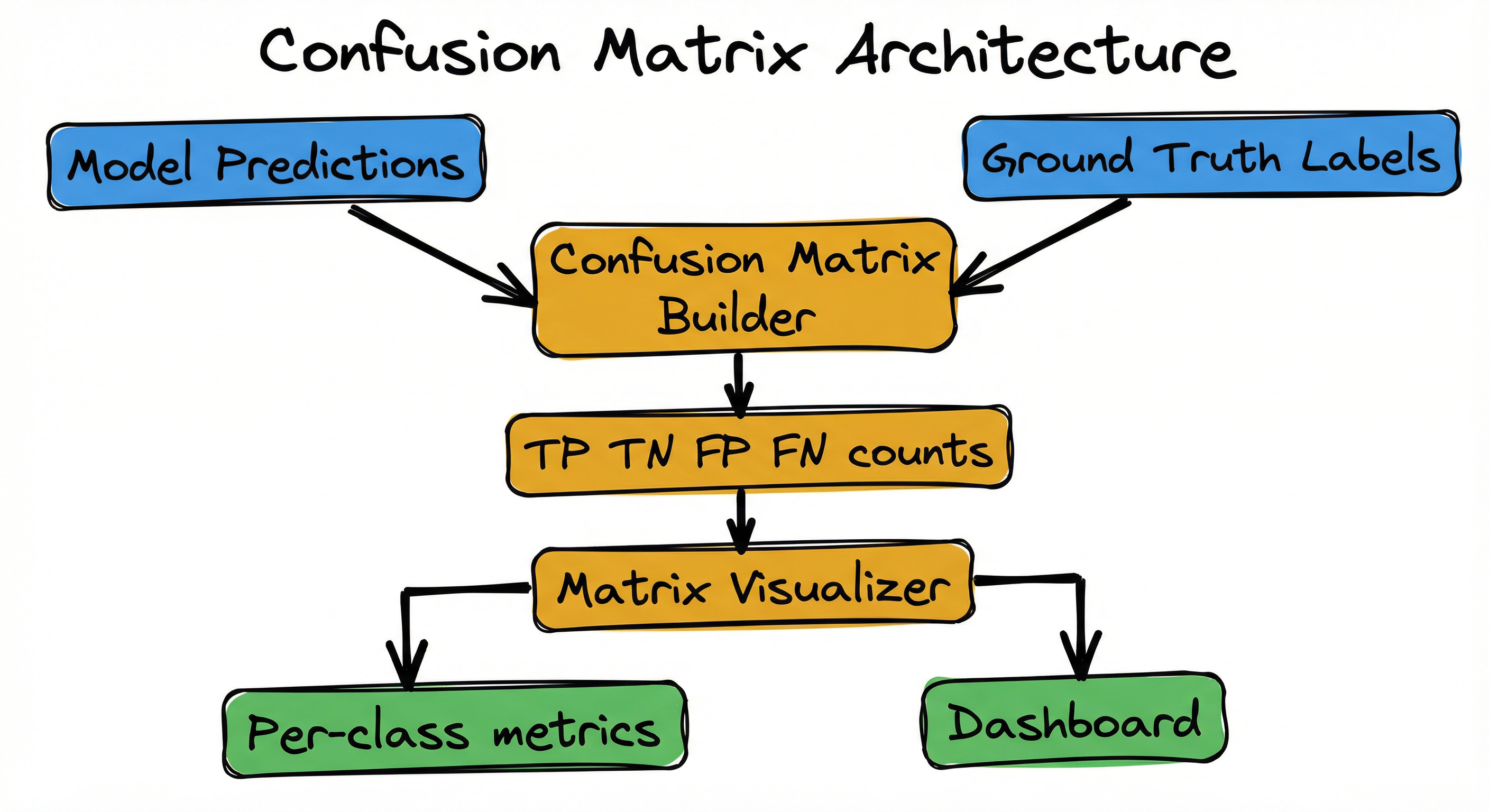
Internal Architecture
A production confusion matrix system consists of four key components: a prediction collector that gathers model outputs and ground truth labels, a matrix computation engine that builds the N×N cross-tabulation, a visualization layer that renders heatmaps and derived metrics, and a monitoring system that tracks matrix changes over time to detect drift.
The architecture supports both batch and streaming modes. In batch mode (typical for model evaluation), the entire test set is processed at once to produce a single confusion matrix. In streaming mode (typical for production monitoring), predictions are accumulated in time windows (hourly, daily) and matrices are computed incrementally.
The feedback loop is critical: when specific misclassification patterns emerge (e.g., class A consistently confused with class B), this triggers root cause analysis — inspecting feature distributions, reviewing training data balance, and potentially retraining with targeted data augmentation for the confused classes.
Key Components
Prediction & Label Collector
Ingests model predictions (either class labels or probability vectors converted to labels via argmax) and corresponding ground truth labels. Handles missing labels via partial matrix computation or imputation. Supports batch ingestion from evaluation datasets and streaming ingestion from production inference logs with buffering (typical window: 1000-10000 samples).
Matrix Computation Engine
Builds the confusion matrix by iterating through (true_label, predicted_label) pairs and incrementing . For large datasets, uses sparse matrix representations when is large (e.g., 1000+ classes) and most class pairs never co-occur. Computes per-class TP, FP, FN, TN for metric derivation.
Normalization Module
Applies row, column, or global normalization to convert raw counts into proportions. Row normalization highlights recall per class (what fraction of each true class was correctly predicted). Column normalization highlights precision per class (what fraction of each predicted class was correct). Choice depends on use case: row norm for class balance analysis, column norm for prediction trustworthiness.
Derived Metrics Calculator
Computes accuracy, precision, recall, F1, specificity, balanced accuracy, and Matthews correlation coefficient from the confusion matrix cells. For multi-class, computes both macro-averaged (unweighted mean across classes) and weighted (weighted by class support) versions of each metric. Includes confidence intervals via bootstrap resampling.
Visualization Engine
Renders the confusion matrix as a heatmap using matplotlib or seaborn. Color intensity represents cell values (high=dark/bright, low=light/dim). Supports custom color maps (sequential for raw counts, diverging for normalized). Annotates cells with counts and/or percentages. For matrices larger than 20×20, uses hierarchical grouping or zooming to maintain readability.
Time-Series Monitor
Stores confusion matrices computed at regular intervals (hourly, daily, weekly) in a time-series database (InfluxDB, Prometheus, or custom SQL tables). Computes matrix difference between consecutive time windows to detect drift: . Large changes in off-diagonal elements trigger alerts. Used for A/B testing to compare confusion matrices across model variants.
Alert & Integration Layer
Integrates with monitoring platforms (Grafana, Datadog, New Relic) to visualize confusion matrix heatmaps in production dashboards. Sends alerts when specific error types exceed thresholds (e.g., "false positive rate for fraud class > 5%"). Supports webhook-based integration with incident management systems (PagerDuty, Slack).
Data Flow
Offline Evaluation Path: After model training, evaluation predictions are collected with ground truth labels → matrix computation engine builds the confusion matrix → normalization module applies row/column/global normalization based on analysis goal → visualization engine renders heatmap → derived metrics calculator computes precision, recall, F1 per class → results are logged to MLflow/Weights & Biases for experiment tracking.
Production Monitoring Path: Inference requests generate predictions → predictions are logged with request IDs → ground truth labels are collected asynchronously (e.g., user feedback, downstream validation) and joined with predictions via request ID → time-series monitor accumulates predictions in sliding windows → matrix is recomputed every N minutes/hours → alert layer checks for drift by comparing current matrix against baseline → violations trigger incident workflows.
Error Analysis Loop: Confusion matrix reveals systematic misclassifications (e.g., class A confused with class B at 15% rate) → data scientist inspects feature distributions for confused classes → discovers feature overlap or insufficient training data → applies targeted mitigation: collect more data for confused classes, engineer discriminative features, apply focal loss or class-weighted training → retrain model → re-evaluate confusion matrix → cycle repeats until confusion is below threshold.
A directed flow showing Model Predictions and Ground Truth Labels feeding into a Matrix Builder, which branches to a Normalize decision point. If normalized, it goes to Row/Col/Global Norm; if not, to Raw Counts. Both paths converge to Visualization, which splits to Heatmap Display and Metrics Dashboard. The Matrix Builder also feeds a Time-Series Storage system that connects to Drift Detection, which feeds an Alert System.
How to Implement
Two Primary Approaches
Approach A: Library-based computation — use sklearn's confusion_matrix() function for batch evaluation during training/testing. This is the most common pattern for offline model evaluation, research, and one-off analysis. Pros: simple API, well-tested, integrates with sklearn's ecosystem. Cons: requires all data in memory, no streaming support.
Approach B: Incremental/streaming computation — maintain a running confusion matrix that updates with each prediction-label pair. This is essential for production monitoring where labels arrive asynchronously and you want real-time matrix updates. Pros: constant memory footprint, supports infinite streams. Cons: requires custom implementation or streaming libraries like River.
For production systems at scale (millions of predictions per day), the hybrid approach is common: accumulate predictions in a message queue (Kafka, RabbitMQ), consume in micro-batches (1000-10000 samples), compute confusion matrix per batch, then merge matrices (element-wise addition). This balances latency, throughput, and code simplicity.
Cost Note: Computing a confusion matrix is negligible in cost. For a model with 10 classes processing 1M predictions/day, the compute cost is under INR 10/month (~$0.12). The bottleneck is never matrix computation — it's collecting ground truth labels in production (which often arrive hours or days after predictions) and joining them with predictions (which requires indexed storage like PostgreSQL, Cassandra, or DynamoDB).
import numpy as np
from sklearn.metrics import confusion_matrix, ConfusionMatrixDisplay
import matplotlib.pyplot as plt

# Simulate binary classification results
np.random.seed(42)
y_true = np.random.randint(0, 2, size=1000)
y_pred_probs = y_true + np.random.randn(1000) * 0.3  # Noisy predictions
y_pred = (y_pred_probs > 0.5).astype(int)

# Compute confusion matrix
cm = confusion_matrix(y_true, y_pred)

print("Confusion Matrix (Raw Counts):")
print(cm)
print(f"\nShape: {cm.shape}")
print(f"\nBreakdown:")
print(f"  True Negatives (TN):  {cm[0, 0]}")
print(f"  False Positives (FP): {cm[0, 1]}")
print(f"  False Negatives (FN): {cm[1, 0]}")
print(f"  True Positives (TP):  {cm[1, 1]}")

# Compute derived metrics
tn, fp, fn, tp = cm.ravel()
accuracy = (tp + tn) / (tp + tn + fp + fn)
precision = tp / (tp + fp)
recall = tp / (tp + fn)
f1 = 2 * (precision * recall) / (precision + recall)

print(f"\nDerived Metrics:")
print(f"  Accuracy:  {accuracy:.4f}")
print(f"  Precision: {precision:.4f}")
print(f"  Recall:    {recall:.4f}")
print(f"  F1-Score:  {f1:.4f}")

# Visualize with ConfusionMatrixDisplay
disp = ConfusionMatrixDisplay(confusion_matrix=cm, display_labels=['Negative', 'Positive'])
disp.plot(cmap='Blues', values_format='d')
plt.title('Binary Confusion Matrix')
plt.show()
This example demonstrates the canonical workflow for binary classification evaluation using scikit-learn. The confusion_matrix() function takes true labels and predicted labels and returns a 2×2 numpy array. We use .ravel() to unpack the four values in standard order (TN, FP, FN, TP). The ConfusionMatrixDisplay class provides a convenient visualization method that handles axis labels, color mapping, and cell annotations automatically. The values_format='d' ensures integers are displayed (not scientific notation).
import numpy as np
from sklearn.metrics import confusion_matrix
import seaborn as sns
import matplotlib.pyplot as plt

# Simulate 5-class classification
np.random.seed(42)
n_samples = 1000
n_classes = 5
y_true = np.random.randint(0, n_classes, size=n_samples)
# Inject bias: class 2 often confused with class 3
y_pred = y_true.copy()
confuse_mask = (y_true == 2) & (np.random.rand(n_samples) < 0.25)
y_pred[confuse_mask] = 3

# Compute raw confusion matrix
cm_raw = confusion_matrix(y_true, y_pred)

# Compute normalized confusion matrices
cm_row_norm = confusion_matrix(y_true, y_pred, normalize='true')    # Row normalization
cm_col_norm = confusion_matrix(y_true, y_pred, normalize='pred')    # Column normalization
cm_global_norm = confusion_matrix(y_true, y_pred, normalize='all')  # Global normalization

# Visualize side-by-side
fig, axes = plt.subplots(2, 2, figsize=(14, 12))

# Raw counts
sns.heatmap(cm_raw, annot=True, fmt='d', cmap='Blues',
            xticklabels=range(n_classes), yticklabels=range(n_classes), ax=axes[0, 0])
axes[0, 0].set_title('Raw Counts')
axes[0, 0].set_ylabel('True Label')
axes[0, 0].set_xlabel('Predicted Label')

# Row normalization (recall perspective)
sns.heatmap(cm_row_norm, annot=True, fmt='.2f', cmap='Greens',
            xticklabels=range(n_classes), yticklabels=range(n_classes), ax=axes[0, 1])
axes[0, 1].set_title('Row Normalized (Recall per class)')
axes[0, 1].set_ylabel('True Label')
axes[0, 1].set_xlabel('Predicted Label')

# Column normalization (precision perspective)
sns.heatmap(cm_col_norm, annot=True, fmt='.2f', cmap='Oranges',
            xticklabels=range(n_classes), yticklabels=range(n_classes), ax=axes[1, 0])
axes[1, 0].set_title('Column Normalized (Precision per class)')
axes[1, 0].set_ylabel('True Label')
axes[1, 0].set_xlabel('Predicted Label')

# Global normalization
sns.heatmap(cm_global_norm, annot=True, fmt='.3f', cmap='Purples',
            xticklabels=range(n_classes), yticklabels=range(n_classes), ax=axes[1, 1])
axes[1, 1].set_title('Global Normalized (Overall distribution)')
axes[1, 1].set_ylabel('True Label')
axes[1, 1].set_xlabel('Predicted Label')

plt.tight_layout()
plt.show()

# Identify top misclassifications
print("\nTop 5 Misclassification Patterns (raw counts):")
off_diag_indices = [(i, j, cm_raw[i, j]) for i in range(n_classes) for j in range(n_classes) if i != j]
off_diag_sorted = sorted(off_diag_indices, key=lambda x: x[2], reverse=True)
for i, j, count in off_diag_sorted[:5]:
    print(f"  True class {i} → Predicted class {j}: {count} samples")
This example demonstrates multi-class confusion matrices with all three normalization modes. Row normalization (normalize='true') divides each row by its sum, showing recall per class: "Given actual class i, what fraction was correctly predicted?" Column normalization (normalize='pred') shows precision per class: "Given prediction j, what fraction was actually correct?" Global normalization (normalize='all') shows the overall joint distribution. The code also demonstrates extracting the top misclassification patterns by sorting off-diagonal elements — critical for error analysis and targeted model improvement.
import numpy as np
from collections import defaultdict
import time

class StreamingConfusionMatrix:
    """Incremental confusion matrix for production monitoring."""

    def __init__(self, n_classes: int):
        self.n_classes = n_classes
        self.matrix = np.zeros((n_classes, n_classes), dtype=np.int64)
        self.total_samples = 0

    def update(self, y_true: int, y_pred: int):
        """Update matrix with a single prediction-label pair."""
        if 0 <= y_true < self.n_classes and 0 <= y_pred < self.n_classes:
            self.matrix[y_true, y_pred] += 1
            self.total_samples += 1

    def batch_update(self, y_true_batch: np.ndarray, y_pred_batch: np.ndarray):
        """Update matrix with a batch of predictions."""
        for yt, yp in zip(y_true_batch, y_pred_batch):
            self.update(yt, yp)

    def get_matrix(self, normalize: str = None) -> np.ndarray:
        """Get current confusion matrix, optionally normalized."""
        if normalize == 'row':
            row_sums = self.matrix.sum(axis=1, keepdims=True)
            return self.matrix / np.maximum(row_sums, 1)  # Avoid division by zero
        elif normalize == 'col':
            col_sums = self.matrix.sum(axis=0, keepdims=True)
            return self.matrix / np.maximum(col_sums, 1)
        elif normalize == 'global':
            return self.matrix / max(self.total_samples, 1)
        else:
            return self.matrix.copy()

    def get_metrics(self) -> dict:
        """Compute per-class and aggregate metrics."""
        cm = self.matrix
        n = self.n_classes

        metrics = {'per_class': [], 'macro_avg': {}, 'weighted_avg': {}}

        for i in range(n):
            tp = cm[i, i]
            fp = cm[:, i].sum() - tp
            fn = cm[i, :].sum() - tp
            tn = cm.sum() - tp - fp - fn

            precision = tp / (tp + fp) if (tp + fp) > 0 else 0.0
            recall = tp / (tp + fn) if (tp + fn) > 0 else 0.0
            f1 = 2 * precision * recall / (precision + recall) if (precision + recall) > 0 else 0.0

            metrics['per_class'].append({
                'class': i,
                'precision': precision,
                'recall': recall,
                'f1': f1,
                'support': cm[i, :].sum()
            })

        # Macro average (unweighted)
        metrics['macro_avg']['precision'] = np.mean([m['precision'] for m in metrics['per_class']])
        metrics['macro_avg']['recall'] = np.mean([m['recall'] for m in metrics['per_class']])
        metrics['macro_avg']['f1'] = np.mean([m['f1'] for m in metrics['per_class']])

        # Weighted average (by class support)
        total_support = sum(m['support'] for m in metrics['per_class'])
        metrics['weighted_avg']['precision'] = sum(m['precision'] * m['support'] for m in metrics['per_class']) / total_support
        metrics['weighted_avg']['recall'] = sum(m['recall'] * m['support'] for m in metrics['per_class']) / total_support
        metrics['weighted_avg']['f1'] = sum(m['f1'] * m['support'] for m in metrics['per_class']) / total_support

        return metrics

    def reset(self):
        """Reset matrix to zeros (for new evaluation window)."""
        self.matrix = np.zeros((self.n_classes, self.n_classes), dtype=np.int64)
        self.total_samples = 0

# Example usage: simulating a production fraud detection system
print("=== Streaming Confusion Matrix for Production Monitoring ===")
np.random.seed(42)
scm = StreamingConfusionMatrix(n_classes=3)  # 3 classes: legit, suspicious, fraud

# Simulate 10 batches of predictions arriving over time
for batch_id in range(10):
    # Generate batch
    batch_size = np.random.randint(50, 150)
    y_true = np.random.randint(0, 3, size=batch_size)
    y_pred = y_true.copy()
    # Inject some errors
    error_mask = np.random.rand(batch_size) < 0.15
    y_pred[error_mask] = np.random.randint(0, 3, size=error_mask.sum())

    # Update streaming matrix
    scm.batch_update(y_true, y_pred)

    # Every 3 batches, print current state
    if (batch_id + 1) % 3 == 0:
        print(f"\n--- After batch {batch_id + 1} (Total samples: {scm.total_samples}) ---")
        print("Raw Confusion Matrix:")
        print(scm.get_matrix())

        metrics = scm.get_metrics()
        print(f"\nMacro Avg F1: {metrics['macro_avg']['f1']:.4f}")
        print(f"Weighted Avg F1: {metrics['weighted_avg']['f1']:.4f}")

print("\n=== Final Per-Class Breakdown ===")
metrics = scm.get_metrics()
for m in metrics['per_class']:
    print(f"Class {m['class']}: Precision={m['precision']:.3f}, Recall={m['recall']:.3f}, F1={m['f1']:.3f}, Support={m['support']}")
This production-ready example implements a streaming confusion matrix that updates incrementally as predictions arrive, suitable for real-time monitoring. The StreamingConfusionMatrix class maintains a running matrix and supports both single-sample and batch updates. This is the pattern used by companies like Swiggy (fraud detection), Flipkart (product categorization monitoring), and Razorpay (risk model tracking) to monitor model performance without loading the entire evaluation set into memory. The get_metrics() method computes per-class precision, recall, and F1, plus macro-averaged and weighted-averaged metrics — critical for imbalanced production datasets.
import numpy as np
from sklearn.metrics import confusion_matrix
import pandas as pd
import matplotlib.pyplot as plt
import seaborn as sns

def analyze_confusions(y_true, y_pred, class_names=None, top_k=10):
    """Identify and visualize the most common misclassification patterns."""

    # Compute confusion matrix
    cm = confusion_matrix(y_true, y_pred)
    n_classes = cm.shape[0]

    if class_names is None:
        class_names = [f"Class {i}" for i in range(n_classes)]

    # Extract off-diagonal confusions
    confusions = []
    for i in range(n_classes):
        for j in range(n_classes):
            if i != j and cm[i, j] > 0:
                confusions.append({
                    'true_class': class_names[i],
                    'pred_class': class_names[j],
                    'count': cm[i, j],
                    'percent_of_true': 100 * cm[i, j] / cm[i, :].sum(),
                    'true_idx': i,
                    'pred_idx': j
                })

    # Sort by count
    confusions_df = pd.DataFrame(confusions).sort_values('count', ascending=False)

    print(f"=== Top {top_k} Misclassification Patterns ===")
    print(confusions_df.head(top_k).to_string(index=False))

    # Visualize confusion heatmap with off-diagonal highlighting
    fig, ax = plt.subplots(figsize=(10, 8))

    # Normalize by row for recall perspective
    cm_norm = cm.astype('float') / cm.sum(axis=1)[:, np.newaxis]

    # Create heatmap
    sns.heatmap(cm_norm, annot=cm, fmt='d', cmap='RdYlGn_r',
                xticklabels=class_names, yticklabels=class_names,
                cbar_kws={'label': 'Recall (row-normalized)'}, ax=ax)

    # Highlight top confusions with red boxes
    for idx, row in confusions_df.head(5).iterrows():
        i, j = row['true_idx'], row['pred_idx']
        ax.add_patch(plt.Rectangle((j, i), 1, 1, fill=False, edgecolor='red', lw=3))

    ax.set_title('Confusion Matrix with Top 5 Misclassifications Highlighted (Red Boxes)')
    ax.set_ylabel('True Label')
    ax.set_xlabel('Predicted Label')
    plt.tight_layout()
    plt.show()

    return confusions_df

# Example: Fashion MNIST-like scenario with 10 classes
np.random.seed(42)
class_names = ['T-shirt', 'Trouser', 'Pullover', 'Dress', 'Coat',
               'Sandal', 'Shirt', 'Sneaker', 'Bag', 'Ankle boot']
n_classes = len(class_names)
y_true = np.random.randint(0, n_classes, size=2000)
y_pred = y_true.copy()

# Inject systematic confusions
# Shirts often confused with T-shirts
shirt_idx = 6
tshirt_idx = 0
confuse_mask = (y_true == shirt_idx) & (np.random.rand(2000) < 0.3)
y_pred[confuse_mask] = tshirt_idx

# Pullovers sometimes confused with Coats
pullover_idx = 2
coat_idx = 4
confuse_mask = (y_true == pullover_idx) & (np.random.rand(2000) < 0.2)
y_pred[confuse_mask] = coat_idx

# Random noise
noise_mask = np.random.rand(2000) < 0.05
y_pred[noise_mask] = np.random.randint(0, n_classes, size=noise_mask.sum())

confusions_df = analyze_confusions(y_true, y_pred, class_names=class_names, top_k=10)
This example demonstrates error analysis — the critical step after computing a confusion matrix. Instead of just looking at overall accuracy, we systematically identify which class pairs are most frequently confused. The analyze_confusions() function extracts all off-diagonal cells, sorts them by count, and computes the percentage of each true class that gets misclassified into each predicted class. The visualization highlights the top 5 confusions with red boxes on the heatmap. This analysis directly guides model improvement: if "Shirt" is frequently confused with "T-shirt," you know these classes need better feature discrimination — perhaps additional training data, data augmentation, or class-specific feature engineering.
# Confusion matrix monitoring configuration (YAML)
confusion_matrix_monitor:
  model_id: fraud-detection-v2.5

  computation:
    classes: ['legitimate', 'suspicious', 'fraud']
    normalization: 'row'  # Options: 'row', 'col', 'global', 'none'
    window_size: 10000    # Number of samples per matrix computation
    update_frequency: 300  # Recompute every 300 seconds (5 minutes)

  storage:
    backend: 'postgresql'  # Store time-series of matrices
    table: 'confusion_matrix_history'
    retention_days: 90

  visualization:
    heatmap:
      colormap: 'RdYlGn_r'  # Red=bad, green=good
      annotate: true        # Show counts in cells
      font_size: 10
    dashboard:
      grafana_panel_id: 'cm-heatmap-fraud'
      refresh_interval: 60  # seconds

  derived_metrics:
    - accuracy
    - per_class_precision
    - per_class_recall
    - per_class_f1
    - macro_f1
    - weighted_f1
    - matthews_correlation

  drift_detection:
    enabled: true
    baseline_matrix: 'confusion_matrix_2026_01_baseline.npy'
    comparison_method: 'frobenius_norm'  # Matrix distance metric
    alert_threshold: 0.15  # Trigger alert if norm(current - baseline) > 0.15

  alerts:
    - condition: 'false_positive_rate[fraud] > 0.05'
      severity: 'high'
      channels: ['slack', 'pagerduty']
      message: 'Fraud FP rate exceeded 5% threshold'

    - condition: 'false_negative_rate[fraud] > 0.10'
      severity: 'critical'
      channels: ['slack', 'pagerduty', 'email']
      message: 'Fraud FN rate exceeded 10% threshold'

    - condition: 'confusion[suspicious->fraud] > 100/hour'
      severity: 'medium'
      channels: ['slack']
      message: 'High confusion between suspicious and fraud classes'

  integration:
    mlflow:
      enabled: true
      log_frequency: 'daily'
      artifact_path: 'confusion_matrices/'

    experiment_tracking:
      log_per_class_metrics: true
      log_heatmap_image: true
Common Implementation Mistakes
- ●
Confusing rows and columns: The most common convention is rows = actual/true classes, columns = predicted classes. But some libraries and papers use the opposite convention. Always check the axis labels before interpreting a confusion matrix. Misinterpreting axes leads to backwards conclusions about precision vs. recall.
- ●
Using raw counts for imbalanced datasets: If class A has 10,000 samples and class B has 100 samples, the raw confusion matrix will be visually dominated by class A. Always use row normalization to see per-class recall, which is crucial for understanding performance on minority classes. In Indian fintech (fraud detection at PhonePe, risk scoring at CRED), fraud classes are 0.1-1% of transactions — raw counts are meaningless.
- ●
Ignoring off-diagonal patterns: Focusing only on diagonal elements (correct predictions) misses the story. The off-diagonal tells you which classes get confused with which. If your digit classifier confuses 8 with 3 and 5 with 6, that suggests specific visual features need attention. Systematic off-diagonal patterns are actionable insights.
- ●
Not tracking confusion matrix over time: A confusion matrix is a snapshot. In production, you need time-series of confusion matrices to detect drift. A model that was 95% accurate last month might still be 95% accurate this month, but if the false positives shifted from class A to class B, that's a signal of distribution shift. Store confusion matrices daily and compute matrix differences.
- ●
Forgetting to normalize when computing metrics: If you manually compute precision/recall from the confusion matrix, remember that for multi-class you need per-class metrics. Don't just sum diagonals and off-diagonals globally — that gives micro-averaged metrics which hide per-class disparities. Always compute per-class TP, FP, FN, TN.
- ●
Using confusion matrix for probability calibration assessment: Confusion matrices are computed from hard labels (0 or 1, class A or B). They don't capture probability calibration — whether predicted probabilities match true frequencies. For calibration, use reliability diagrams (calibration curves) or Brier score, not confusion matrices.
- ●
Visualizing 100x100 matrices without aggregation: If you have 100+ classes (product categories at Flipkart, language detection, molecular classification), a 100×100 heatmap is unreadable. Either aggregate into class groups, use hierarchical confusion matrices, or show only the top-K most confused classes. Don't render the full matrix blindly.
When Should You Use This?
Use When
Your model performs classification (binary or multi-class) and you need to understand which types of errors it makes, not just overall accuracy
You are evaluating models with class imbalance where minority classes matter (fraud detection, rare disease diagnosis, anomaly detection) — confusion matrix reveals per-class performance that accuracy hides
You need to diagnose systematic misclassifications — if your product categorization model frequently confuses "laptop" with "tablet," the confusion matrix shows this pattern immediately
You are comparing multiple model variants (A/B testing) and need granular error analysis — comparing confusion matrices side-by-side reveals which model makes which types of errors
Your model operates in production and you need to monitor drift — tracking confusion matrices over time detects changes in error patterns before overall accuracy degrades
You are optimizing a decision threshold and need to understand the precision-recall tradeoff — sweeping thresholds and plotting confusion matrices for each reveals the optimal operating point
You need to communicate model performance to non-technical stakeholders — a heatmap is more intuitive than a table of metrics for product managers and executives
Avoid When
Your task is regression, not classification — confusion matrices apply only to discrete class predictions, not continuous outputs. Use residual plots, MAE, RMSE for regression.
You have 1000+ classes with sparse predictions (most class pairs never co-occur) — the N×N matrix becomes too large to store or visualize effectively. Use per-class precision/recall metrics or hierarchical aggregation instead.
You care only about ranking quality, not hard classification decisions (e.g., search result ranking, recommendation systems) — use ranking metrics like NDCG, MAP, MRR. Confusion matrices require hard labels.
Your labels are probabilistic or noisy — if ground truth is inherently uncertain (e.g., human-labeled sentiment from crowdsourcing with low agreement), the confusion matrix will reflect label noise, not model error. Consider multi-rater metrics or label confidence weighting.
You need to assess probability calibration — confusion matrices use hard labels (argmax of probabilities) and discard calibration information. Use reliability diagrams or expected calibration error (ECE) instead.
Key Tradeoffs
The Normalization Decision: Row, Column, or Global?
The choice of normalization fundamentally changes what the confusion matrix reveals:
| Normalization | What It Shows | Best For | Pitfall |
|---|---|---|---|
| Row (normalize='true') | Per-class recall: "Of all actual class i samples, what fraction was correctly predicted?" | Understanding model performance per true class, especially with imbalanced data. Essential for medical diagnosis ("Did we catch all cancer cases?"). | Hides overall class distribution. Can make a rare class look good (100% recall) when it has only 3 samples total. |
| Column (normalize='pred') | Per-class precision: "Of all predictions for class j, what fraction was correct?" | Understanding prediction trustworthiness. If the model predicts "fraud," how often is it actually fraud? Critical for minimizing false alarms. | Hides recall. A model that rarely predicts a class can have artificially high column-normalized values. |
| Global (normalize='all') | Joint distribution: Each cell shows what fraction of all samples fall into that (true, pred) combination. | Understanding overall error distribution when classes are balanced. Good for theoretical analysis. | Useless for imbalanced data — minority classes vanish into rounding errors. |
| None (raw counts) | Absolute sample counts | Debugging, understanding sample sizes, verifying data integrity. | Dominated by majority classes. Visually misleading for imbalanced datasets. |
Rule of thumb: For imbalanced classification (fraud, rare diseases, anomalies), always use row normalization first to see per-class recall. Then check column normalization to understand precision. Never rely on raw counts alone.
Memory and Compute: When Does It Break?
Confusion matrix computation is in samples and in classes. For typical ML:
- 10 classes, 1M samples: Matrix is 10×10 = 100 cells. Storage: ~400 bytes. Compute time: <10ms. No problem.
- 1000 classes, 1M samples: Matrix is 1000×1000 = 1M cells. Storage: ~4MB. Compute time: ~50ms. Still fine.
- 10,000 classes, 1B samples: Matrix is 10K×10K = 100M cells. Storage: ~400MB. Compute time: ~5 seconds. Borderline — use sparse matrices if most class pairs never co-occur.
- 100,000+ classes (extreme multi-label classification, open-vocabulary language models): Full confusion matrix is infeasible. Use per-class metrics without building the full matrix.
For Flipkart's product categorization (40M products, ~20K categories), storing the full 20K×20K confusion matrix is reasonable (~1.6GB at float32). For extreme scenarios like YouTube video classification (millions of possible labels), confusion matrices are not practical.
Pros, Cons & Tradeoffs
Advantages
Reveals error patterns, not just error rates — shows which classes get confused with which, enabling targeted model improvement (collect more data for confused classes, engineer discriminative features, adjust class weights)
Intuitive visual interpretation — a heatmap is immediately understandable even to non-technical stakeholders. Bright off-diagonal spots visually scream "this is where the model fails"
Supports asymmetric cost analysis — in fraud detection at Razorpay or PhonePe, false positives (blocking legitimate transactions) and false negatives (missing fraud) have different business costs. The confusion matrix lets you see and optimize each separately
Essential for imbalanced datasets — when rare classes matter (0.1% fraud among 99.9% legitimate transactions), accuracy is meaningless. Row-normalized confusion matrix shows per-class recall, the metric that actually matters
Foundation for all classification metrics — precision, recall, F1, specificity, sensitivity, balanced accuracy, MCC — all computed from confusion matrix cells. Understanding the matrix means understanding everything downstream
Production monitoring workhorse — tracking confusion matrices over time (daily, hourly) detects drift and data quality issues before accuracy degrades. A sudden spike in specific off-diagonal cells signals actionable problems
Language and framework agnostic — every ML platform and library supports confusion matrices (sklearn, TensorFlow, PyTorch, MLflow, Weights & Biases). It's the universal standard for classification evaluation
Disadvantages
Requires ground truth labels — in production, true labels often arrive hours or days after predictions (e.g., user feedback, downstream validation). You cannot compute a confusion matrix until labels are available, creating a monitoring delay. This is the single biggest practical limitation.
Becomes unwieldy for 100+ classes — a 100×100 heatmap is visually overwhelming and computationally expensive to render. For extreme multi-class scenarios (product categories at Amazon, language detection for 100+ languages), the full matrix is impractical. Requires hierarchical aggregation or per-class metrics.
Does not capture probability calibration — confusion matrices use hard labels (0 or 1, class A or B). If your model outputs well-calibrated probabilities, the confusion matrix discards that information. Use reliability diagrams or Brier score to assess calibration.
Sensitive to threshold choice — for probabilistic classifiers, the confusion matrix depends on the decision threshold (typically 0.5 for binary). A different threshold produces a different matrix. ROC and PR curves show performance across all thresholds; confusion matrix shows only one.
Can be misleading with extreme imbalance — if one class has 999,999 samples and another has 1 sample, the raw confusion matrix is visually dominated by the majority class. Row normalization fixes this, but many practitioners forget to normalize and draw wrong conclusions from raw counts.
No information about prediction confidence — a confident correct prediction looks the same as a barely-correct prediction in the confusion matrix. If your model predicted class A with 51% probability vs. 99% probability, the matrix treats them identically. Consider examining probability distributions alongside the matrix.
Failure Modes & Debugging
Label delay in production causing monitoring blindness
Cause
In production systems, predictions are logged in real-time but ground truth labels arrive asynchronously — often hours or days later (user feedback, downstream validation, manual review). For example, a Swiggy fraud model logs predictions instantly, but confirmation of fraud (chargeback, investigation) takes 2-7 days. This creates a monitoring delay: you cannot compute an accurate confusion matrix until labels arrive.
Symptoms
Confusion matrix dashboard shows stale data (hours/days behind real-time). Model drift or data quality issues go undetected until label delay period expires. By the time you detect elevated false positives, thousands of users have already been affected. Time-series plots show gaps or low sample counts in recent windows.
Mitigation
Implement partial matrix monitoring using available labels (even if incomplete) and clearly indicate sample size and label availability lag. Use proxy metrics that don't require labels (prediction distribution shift, feature distribution drift) to get early signals. For critical applications, implement accelerated labeling (human review of samples, prioritized label collection). Log prediction IDs and implement join logic to retroactively update confusion matrices when labels arrive.
Row/column confusion leading to wrong metric interpretation
Cause
There are two common conventions for confusion matrix orientation: (1) rows=actual, columns=predicted, and (2) rows=predicted, columns=actual. Different libraries and papers use different conventions. When interpreting a confusion matrix from an unfamiliar source, practitioners sometimes get the axes backwards, leading to swapped precision/recall interpretations.
Symptoms
A team reports "high precision, low recall" but the actual pattern is the opposite. Mitigation strategies that target false positives end up targeting false negatives instead. Confusion between stakeholders when discussing the same matrix plotted with different orientations. Debugging takes hours before someone notices the axis labels.
Mitigation
Always explicitly label axes on confusion matrix plots with "True Label" and "Predicted Label" (not just generic "Actual" and "Predicted"). Establish organization-wide conventions and document them in your ML platform's style guide. In code, verify orientation by checking a known error pattern: if you deliberately inject a false positive, does it appear where you expect? Use sklearn's ConfusionMatrixDisplay which enforces the standard convention (rows=true, columns=pred).
Sparse classes with zero true samples causing metric explosions
Cause
In multi-class classification with rare classes, evaluation datasets may have zero samples for some classes purely by chance. When computing per-class metrics (precision = TP/(TP+FP), recall = TP/(TP+FN)), division by zero occurs. This is especially common in long-tail distributions (e-commerce product categories, rare diseases, infrequent events).
Symptoms
Metrics computation crashes with division by zero errors. Or worse, libraries return NaN or inf values that propagate through calculations, producing misleading macro-averaged metrics. Per-class F1 scores show nonsensical values (NaN, inf, or 0.0 for all metrics despite the model clearly making predictions for that class).
Mitigation
Use epsilon smoothing: add a small constant (typically 1e-10) to denominators to avoid division by zero. In sklearn, many functions have a zero_division parameter (set to 0, 1, or 'warn'). For production monitoring, explicitly filter out classes with zero support before computing metrics and report them separately. Document minimum sample size requirements (e.g., "require N≥30 per class for reliable metrics"). For rare classes, aggregate over longer time windows to accumulate sufficient samples.
Threshold drift causing confusion matrix shift without accuracy change
Cause
For probabilistic classifiers, predictions are converted to hard labels using a threshold (e.g., pred_class = 1 if prob ≥ 0.5 else 0). If the model's probability calibration drifts over time — perhaps due to distribution shift or feature drift — the effective threshold changes even if the nominal threshold stays at 0.5. This can shift false positives to false negatives (or vice versa) while maintaining the same total error rate.
Symptoms
Overall accuracy remains stable (±1%), but confusion matrix shows dramatic shifts in off-diagonal elements. False positive rate doubles while false negative rate drops by half. Business impact changes (more customer complaints about blocked transactions vs. more fraud losses) even though ML metrics look fine. Users report "the model feels different" despite stable accuracy.
Mitigation
Monitor predicted probability distributions alongside confusion matrices using histograms or KDE plots. Detect calibration drift using calibration curves or expected calibration error (ECE) computed on a fixed calibration set. Implement probability calibration using Platt scaling or isotonic regression, and periodically recalibrate in production. Log both hard labels and probabilities so you can retroactively adjust thresholds during analysis. Alert on mean predicted probability drift, not just accuracy.
Data leakage via temporal features making confusion matrix artificially perfect
Cause
During training or evaluation, temporal features (timestamps, order IDs, sequence numbers) that correlate perfectly with labels leak information. For example, in a fraud detection dataset, if fraudulent transactions systematically occur after midnight and legitimate ones during business hours, a "time_of_day" feature will perfectly separate classes. The confusion matrix will show near-perfect diagonal, but the model will fail in production when fraud patterns shift.
Symptoms
Training confusion matrix shows 99%+ accuracy with near-perfect diagonal. Test set confusion matrix also looks perfect. But production confusion matrix immediately degrades to 60-70% accuracy. Large gap between offline evaluation and online performance. Model gives high confidence predictions during evaluation but low confidence in production.
Mitigation
Perform temporal validation: train on time period T1, evaluate on T2 (future holdout), then on T3 (even further future). Confusion matrices should remain stable across time windows. Use feature importance analysis (SHAP, permutation importance) to detect if any single feature dominates predictions. Deliberately test on adversarial datasets where temporal patterns differ from training. Establish a policy: any model with >95% test accuracy triggers mandatory leakage investigation.
Placement in an ML System
Where Does It Sit in the Pipeline?
The confusion matrix operates at two distinct points in the ML lifecycle:
Point 1: Offline Evaluation (Post-Training) — After training, the model is evaluated on a held-out test set (or validation set during development). Predictions are generated for all test samples, the confusion matrix is computed, and derived metrics (precision, recall, F1) are calculated. This is the primary quality gate for deciding whether to promote the model to production. The confusion matrix is logged to experiment tracking platforms (MLflow, Weights & Biases) alongside hyperparameters, training loss curves, and other artifacts. This is analogous to unit tests in software engineering.
Point 2: Production Monitoring (Post-Deployment) — In production, the model serves real traffic. Predictions are logged continuously. Ground truth labels are collected asynchronously (user feedback, downstream validation, manual review). Confusion matrices are computed in time windows (hourly, daily) and stored in time-series databases (InfluxDB, Prometheus, or PostgreSQL with TimescaleDB extension). Dashboards visualize confusion matrices in real-time, and alerts trigger when off-diagonal elements exceed thresholds or when matrix differences (current vs. baseline) exceed drift limits. This is analogous to runtime health checks and APM (application performance monitoring).
Key Insight: The offline confusion matrix tells you if the model was good at a point in time. The production confusion matrix tells you if the model remains good as data distributions shift. Most teams focus only on offline evaluation and neglect production monitoring — a critical mistake. Models degrade in production due to concept drift, data drift, and adversarial behavior. Continuous confusion matrix monitoring is the only way to detect this degradation early.
Pipeline Stage
Evaluation / Monitoring
Upstream
- model-training
- model-inference
- data-validation
Downstream
- metrics-collector
- drift-detection
- alerting
- model-registry
Scaling Bottlenecks
Confusion matrix computation itself scales linearly with samples () and quadratically with classes ( memory). For most ML systems, this is not a bottleneck:
Typical scenario (Flipkart product categorization): 1M predictions/day, 20K classes → 20K×20K matrix = 400M cells × 4 bytes = 1.6GB per day. Storing daily matrices for 90 days = 144GB. Manageable with cloud object storage (INR 2,000/month on AWS S3, ~$24/month).
Extreme scenario (YouTube video classification): 100M predictions/day, 1M classes → 1M×1M matrix = 1 trillion cells × 4 bytes = 4TB per matrix. Infeasible. Must use sparse matrices (most class pairs never co-occur) or hierarchical aggregation.
The real scaling bottlenecks are not computation:
1. Label collection at scale: For a Swiggy fraud model with 10M predictions/day, collecting ground truth for every prediction is impossible. Typically only 1-10% of predictions get labels (user reports, manual reviews). This creates sparse, biased samples for the confusion matrix. Mitigation: stratified sampling, importance sampling (prioritize high-uncertainty predictions for labeling).
2. Joining predictions with delayed labels: Predictions are logged with request IDs. Labels arrive asynchronously (hours/days later) and must be joined via request ID. At 10M predictions/day, this requires indexed storage (PostgreSQL with BTREE index, Cassandra with partition keys, or DynamoDB with sort keys). Join queries can become bottlenecks. Cost: INR 20,000-50,000/month (~$250-600/month) for managed database at this scale.
3. Real-time visualization for 1000+ classes: Rendering a 1000×1000 heatmap in a Grafana dashboard at 1-second refresh requires client-side GPU acceleration or server-side prerendering. Most web browsers choke on >100×100 heatmaps with real-time updates. Mitigation: hierarchical zoom (show 10×10 class groups, drill down to full resolution), or show only top-K confused classes.
Production Case Studies
Gmail's spam filter processes billions of emails daily with a binary classification model (spam vs. not spam). Google uses confusion matrices to monitor false positive rate (legitimate email marked as spam) and false negative rate (spam reaching inbox). The FP rate is the critical metric — users are far more frustrated by missing important emails than by occasional spam leakage. Google maintains FP rate <0.05% by continuously monitoring confusion matrices, setting strict thresholds, and retraining when drift is detected.
Gmail spam filter maintains 99.9%+ accuracy with <0.05% FP rate by using confusion matrix monitoring to detect drift within minutes. The system processes real-time confusion matrices on 10-minute windows, comparing against baseline matrices to trigger alerts. This architecture became the blueprint for production classification monitoring across Google.
Flipkart's product categorization system classifies 40M+ products into ~20,000 hierarchical categories using a combination of text (title, description) and image features. The confusion matrix reveals systematic misclassifications: "men's running shoes" confused with "men's sports shoes," "laptop bags" confused with "backpacks." The normalized confusion matrix (row normalization) shows per-category recall, highlighting categories with <80% recall that need more training data or better features.
By analyzing confusion matrix patterns, Flipkart identified 150 frequently-confused category pairs and applied targeted fixes: collected additional training data for those pairs, engineered discriminative features (brand name, price range), and applied focal loss during training to emphasize hard examples. Category-wise F1 improved from 78% to 89% average.
Apollo Hospitals deployed an AI system for diabetic retinopathy screening in rural India, classifying retinal images into 5 severity levels (no DR, mild, moderate, severe, proliferative DR). The confusion matrix revealed a critical failure mode: the model frequently confused severe DR with moderate DR (17% false negative rate for severe cases). This is catastrophic — severe cases need immediate referral to prevent blindness. Apollo used the confusion matrix to identify this specific error pattern and retrained with class-weighted loss, oversampling severe cases.
After targeted retraining guided by confusion matrix analysis, false negative rate for severe DR dropped from 17% to 4.2%. The system now screens 50,000+ patients annually in rural clinics, with confusion matrices monitored weekly to ensure the severe DR → moderate DR confusion remains below 5% threshold.
Razorpay's technical blog explains their ML-based fraud detection approach, processing millions of transactions daily using classification models that must make decisions in milliseconds, leveraging Apache Flink for real-time feature generation and XGBoost for classification.
Built Mitra data intelligence platform based on Kappa+ architecture with Apache Flink as core engine and RocksDB for in-memory states, enabling real-time fraud detection at scale for India's leading payment processor.
Tooling & Ecosystem
The canonical Python library for confusion matrix computation. Supports binary and multi-class classification, normalization (row, column, global), and sample weighting. The ConfusionMatrixDisplay class provides matplotlib-based visualization with customizable colormaps and annotations. Works seamlessly with sklearn classifiers and pipelines.
High-level statistical visualization library built on matplotlib. The heatmap() function is the go-to for confusion matrix visualization, offering extensive customization: color palettes (sequential, diverging), annotations (counts, percentages, custom formats), cell sizes, and hierarchical clustering. Produces publication-quality heatmaps with minimal code.
TensorFlow's tf.math.confusion_matrix() computes confusion matrices from tensors, integrating natively with TensorFlow/Keras training loops. Supports GPU acceleration for large batch computation. The tf.keras.metrics module includes Precision, Recall, AUC which can be tracked during training, though the full confusion matrix is typically computed post-training.
Open-source ML lifecycle platform with built-in support for logging confusion matrices as artifacts. Use mlflow.log_figure() to store matplotlib/seaborn heatmaps, or mlflow.log_dict() to store the raw matrix as JSON/YAML. The MLflow UI displays confusion matrices alongside metrics, parameters, and model artifacts, enabling easy comparison across experiments.
Experiment tracking platform with first-class support for confusion matrices. Use wandb.log({"conf_mat": wandb.plot.confusion_matrix(...)}) to log interactive heatmaps that support zooming, filtering by class, and time-series comparison across training runs. Particularly strong for tracking confusion matrix evolution during training (epoch-by-epoch or batch-by-batch).
Open-source Python library for ML model monitoring and evaluation, with extensive confusion matrix analysis built-in. Generates interactive HTML reports showing confusion matrices with normalization, per-class metrics, and drift detection (comparing confusion matrices across time windows). Designed specifically for production ML monitoring use cases.
Interactive visualization library for creating web-based confusion matrix heatmaps with hover tooltips, zooming, and panning. Produces standalone HTML files or integrates with Dash dashboards. Particularly useful for large confusion matrices (50+ classes) where interactivity helps navigate the matrix.
Visual analysis and diagnostic library extending sklearn. The ConfusionMatrix visualizer integrates directly with sklearn estimators, automatically computing and plotting confusion matrices with class labels, normalization, and derived metrics. Simplifies the workflow for sklearn users who want publication-ready visualizations without manually calling matplotlib/seaborn.
Research & References
Okolie, J.A., et al. (2024)African Journal of Biomedical Research
Comprehensive survey of confusion matrix-based metrics for classification evaluation. Covers accuracy, precision, recall, F1, specificity, sensitivity, balanced accuracy, and Matthews correlation coefficient. Emphasizes the importance of choosing appropriate metrics for imbalanced datasets, particularly in medical diagnostics where false negatives carry higher cost than false positives.
Janocha, K., Czarnecki, W.M. (2023)Journal of the Royal Statistical Society Series C
Introduces hierarchical confusion matrices for taxonomic and structured classification problems (e.g., product categories, biological classification). Enables evaluation at multiple levels of granularity: fine-grained (leaf nodes) vs. coarse-grained (parent categories). Shows that standard confusion matrices hide hierarchical misclassification costs — confusing "dog" with "cat" is less severe than confusing "dog" with "car."
Chicco, D., Jurman, G. (2021)BioData Mining
Empirical study demonstrating that Matthews Correlation Coefficient (MCC) is more robust than balanced accuracy and other confusion matrix-derived metrics for imbalanced classification. MCC considers all four confusion matrix cells (TP, TN, FP, FN) proportionally and produces high scores only when the classifier performs well across all categories. Recommends MCC as the standard metric for evaluating binary classifiers in genomics, proteomics, and medical diagnostics.
Branco, P., et al. (2025)arXiv preprint
Proposes a universal standardization method for confusion matrix-based metrics that maps them to a common [0,1] scale and enables meaningful comparison across datasets with differing class imbalance. The outperformance score function adjusts for random guessing baseline, making it possible to compare precision, recall, F1, and MCC across experiments with different prevalence. Particularly relevant for meta-analysis and model selection across heterogeneous datasets.
Luque, A., et al. (2019)Pattern Recognition
Systematic analysis of how class imbalance affects confusion matrix-derived metrics (accuracy, precision, recall, F1, MCC). Shows that accuracy is highly misleading when imbalance ratio exceeds 10:1, while MCC remains stable. Provides empirical guidelines for metric selection based on imbalance ratio and cost asymmetry. Essential reading for practitioners working with rare-event classification (fraud, disease diagnosis, anomaly detection).
Reis, H.C., et al. (2024)Technologies (MDPI)
Introduces probabilistic confusion matrices that incorporate prediction uncertainty (confidence scores) rather than treating all predictions as equally certain. Computes expected confusion matrices by weighting each prediction by its probability distribution over classes. Enables more nuanced performance evaluation for models that output calibrated probabilities, showing when a model is confidently wrong vs. uncertainly wrong.
Interview & Evaluation Perspective
Common Interview Questions
- ●
Explain the difference between precision and recall using a confusion matrix. When would you optimize for one over the other?
- ●
How would you interpret a confusion matrix for a multi-class classification problem? Walk me through an example.
- ●
A binary classifier has 95% accuracy, but the confusion matrix shows 99% of predictions are for the negative class. What's going on and how do you fix it?
- ●
How would you monitor a classification model in production using confusion matrices? What metrics would you track and what thresholds would you set?
- ●
You have a 1000-class classification problem. Is it practical to compute and visualize the full confusion matrix? If not, what alternatives would you use?
- ●
Explain normalization in confusion matrices. When would you use row normalization vs. column normalization?
- ●
How would you use a confusion matrix to diagnose class imbalance in your training data?
Key Points to Mention
- ●
The confusion matrix is the foundation for all classification metrics — precision, recall, F1, accuracy, specificity, MCC all derive from its four cells (TP, TN, FP, FN). Understanding the matrix means understanding everything downstream.
- ●
Row normalization (normalize='true') shows per-class recall, answering "Given actual class i, what fraction was correctly predicted?" This is critical for imbalanced datasets where you care about minority class detection.
- ●
Column normalization (normalize='pred') shows per-class precision, answering "Given prediction j, what fraction was actually correct?" This is critical when false alarms have high cost (e.g., fraud detection, spam filtering).
- ●
In production, confusion matrices should be monitored over time (time-series of matrices) to detect drift. A sudden shift in off-diagonal elements signals distribution shift, data quality issues, or adversarial behavior before overall accuracy degrades.
- ●
For imbalanced classification (fraud, rare disease, anomaly detection), accuracy is meaningless. The confusion matrix reveals per-class performance that aggregate metrics hide. Always compute and report per-class precision, recall, and F1.
- ●
Matthews Correlation Coefficient (MCC) is the most robust single-number metric for imbalanced classification, as it considers all four confusion matrix cells proportionally. Range [-1, +1], with 0 indicating random performance.
Pitfalls to Avoid
- ●
Confusing rows and columns — always verify the convention (rows=true, columns=pred is standard in sklearn). Getting axes backwards leads to swapped precision/recall interpretation.
- ●
Using raw counts for imbalanced data — raw counts are visually dominated by majority classes. Always use row normalization to see per-class recall for imbalanced datasets.
- ●
Ignoring off-diagonal patterns — the off-diagonal tells the story. Systematic confusions (class A frequently mistaken for class B) are actionable insights for model improvement.
- ●
Treating confusion matrix as a static snapshot — in production, models drift. Track confusion matrices over time and alert on matrix differences (Frobenius norm, KL divergence) to detect drift.
- ●
Forgetting that confusion matrices require ground truth labels — in production, labels arrive asynchronously (hours/days later). Account for label delay in monitoring architecture.
Senior-Level Expectation
A senior candidate should demonstrate understanding of the full lifecycle of confusion matrix usage: offline evaluation (single matrix per experiment, logged to MLflow/W&B), online monitoring (time-series of matrices, drift detection, alerting), and error analysis (extracting misclassification patterns to guide model improvement). They should discuss normalization strategies and when to use each (row for recall, column for precision), handling class imbalance (weighted metrics, stratified sampling), and scaling challenges (sparse matrices for 1000+ classes, label delay in production, join complexity). They should articulate the business context: why false positives and false negatives have different costs (fraud detection, medical diagnosis, spam filtering), how to set thresholds based on business impact, and how to communicate confusion matrix insights to non-technical stakeholders using heatmaps and derived metrics. For Indian context, they should discuss real-world examples: Flipkart product categorization (20K classes), Swiggy fraud detection (asymmetric FP/FN costs), Razorpay risk scoring (real-time monitoring). They should also know when not to use confusion matrices: regression problems, ranking tasks (use NDCG), probability calibration assessment (use reliability diagrams). Finally, they should discuss advanced topics: hierarchical confusion matrices for taxonomic classification, probabilistic confusion matrices incorporating prediction confidence, and confusion matrix-based active learning (prioritize labeling of frequently-confused classes).
Summary
The confusion matrix is the foundational diagnostic tool for classification evaluation, providing a tabular breakdown of how predictions align with ground truth labels across all classes. While accuracy collapses performance into a single number, the confusion matrix reveals the full picture: which classes the model predicts accurately (diagonal elements) and which classes it confuses with which (off-diagonal elements). This granular view is essential for understanding model behavior, diagnosing failure modes, and guiding targeted improvements.
For binary classification, the 2×2 confusion matrix decomposes accuracy into four components: true positives (TP), true negatives (TN), false positives (FP), and false negatives (FN). From these four values, we derive all standard classification metrics — precision (), recall (), F1 (), specificity, and Matthews correlation coefficient. For multi-class classification, the matrix expands to N×N, with per-class TP, FP, FN, TN computed from matrix cells to enable per-class metric calculation.
Normalization transforms raw counts into proportions, with three modes serving different analytical goals: row normalization (per-class recall, essential for imbalanced data), column normalization (per-class precision, critical for understanding prediction trustworthiness), and global normalization (overall joint distribution). The choice of normalization fundamentally changes interpretation — row norm answers "Given actual class i, what fraction was correctly predicted?" while column norm answers "Given prediction j, what fraction was correct?"
In production ML systems at companies like Flipkart (product categorization), Swiggy (fraud detection), and Razorpay (risk scoring), confusion matrices transition from static evaluation tools to time-series monitoring systems. Matrices are computed in sliding windows (hourly, daily), stored in time-series databases, and visualized in dashboards (Grafana, Datadog). Drift detection compares current matrices against baseline using matrix distance metrics (Frobenius norm, KL divergence), triggering alerts when off-diagonal elements shift significantly. This continuous monitoring catches model degradation, data drift, and adversarial behavior before overall accuracy declines.
The tooling ecosystem is mature: scikit-learn provides the canonical confusion_matrix() function and ConfusionMatrixDisplay for visualization, seaborn offers publication-quality heatmaps with extensive customization, and MLflow/Weights & Biases enable experiment tracking and comparison. For production monitoring, Evidently AI specializes in confusion matrix-based drift detection, while Prometheus/InfluxDB store time-series of matrices for long-term analysis.