Log Loss in Machine Learning
Log loss -- also called binary cross-entropy or negative log-likelihood -- is the gold-standard metric for evaluating classifiers that output probabilities rather than hard class labels. While accuracy tells you "what percentage of predictions were correct," log loss tells you "how confident was the model, and was that confidence justified?"
Consider two classifiers predicting whether a Swiggy order will be delivered late. Classifier A predicts 0.51 probability for a late delivery that actually happened. Classifier B predicts 0.99 for the same event. Both are "correct" if you threshold at 0.5, so both score equally under accuracy. But log loss rewards Classifier B massively -- it was not only right, it was right with conviction. A model that says "I'm 99% sure" and turns out to be correct is fundamentally more useful than one that says "I'm 51% sure" and happens to be correct.
This distinction between hard classification and probabilistic evaluation is why log loss is the default loss function for logistic regression, the optimization objective for nearly every neural network classifier, and the primary evaluation metric in machine learning competitions on platforms like Kaggle. In production systems -- from Razorpay's fraud scoring to PhonePe's credit risk models -- decisions downstream of the classifier depend on calibrated probability estimates, not just binary labels. Log loss directly measures the quality of those probability estimates.
This guide covers the mathematical foundations, the deep connection to information theory and maximum likelihood estimation, practical implementation with scikit-learn and TensorFlow, calibration diagnostics, multi-class extensions, comparison with alternatives like Brier score and AUC-ROC, failure modes that silently wreck production systems, and real-world case studies from Indian and global tech companies.
Concept Snapshot
- What It Is
- A metric that measures the quality of probabilistic predictions by penalizing confident wrong predictions heavily and rewarding confident correct predictions, calculated as the negative average log-probability assigned to the true class labels.
- Category
- Evaluation
- Complexity
- Intermediate
- Inputs / Outputs
- Inputs: predicted probability distributions over classes and true class labels. Outputs: a single non-negative scalar where 0 represents perfect prediction (all true labels assigned probability 1.0), and higher values indicate worse predictions.
- System Placement
- Sits in the model evaluation stage after a classifier produces probability outputs on a validation or test set. Used for model selection, hyperparameter tuning, and as the optimization objective during training (cross-entropy loss).
- Also Known As
- Binary cross-entropy, Cross-entropy loss, Negative log-likelihood, Logarithmic loss, Logistic loss, Log-likelihood loss
- Typical Users
- Data Scientists, ML Engineers, Risk Analysts, Actuaries, Research Scientists, Kaggle Competitors
- Prerequisites
- Probability basics (0-1 range, probability distributions), Logarithms (natural log properties), Binary and multiclass classification, Confusion matrix and accuracy, Maximum likelihood estimation (helpful, not required)
- Key Terms
- binary cross-entropynegative log-likelihoodprobability calibrationBrier scoreproper scoring ruleKL divergencesoftmaxsigmoidlabel smoothingexpected calibration error
Why This Concept Exists
The Problem with Hard Labels
Accuracy, precision, recall, and F1 all operate on hard class labels -- the model either predicted the right class or it didn't. But most modern classifiers (logistic regression, neural networks, gradient boosted trees, etc.) naturally produce probability estimates before those estimates are thresholded into hard labels. Reducing a rich probability distribution to a binary 0/1 decision discards valuable information about the model's uncertainty.
Consider a credit scoring model at a fintech company like Lendingkart or Slice. A customer with a 52% default probability and one with a 98% default probability are both classified as "likely to default" under a 50% threshold. But the lending decision should be very different: you might offer the 52% customer a smaller loan with a higher interest rate, while outright rejecting the 98% customer. Accuracy treats both predictions identically; log loss distinguishes them by rewarding well-calibrated confidence.
Historical Roots in Information Theory
Log loss has deep roots in information theory and maximum likelihood estimation, dating back to Claude Shannon's foundational work on entropy in 1948. Shannon showed that the optimal encoding length for an event with probability is bits. When a model assigns probability to an event that occurs with true probability , the cross-entropy measures the inefficiency of using the model's distribution instead of the true distribution.
This theoretical foundation gives log loss a special property: it is a strictly proper scoring rule. A proper scoring rule is one where the expected score is minimized (or maximized, depending on convention) when the model's predicted probabilities exactly match the true probabilities. In plain terms, a model cannot "game" log loss by outputting anything other than its true belief -- misrepresentation always increases the expected loss. Accuracy, by contrast, is not a proper scoring rule: a model can sometimes improve its accuracy by deliberately outputting overconfident predictions.
From Theory to Training Objective
Log loss's mathematical properties made it the natural choice as the loss function for training classifiers. Logistic regression minimizes log loss directly (that's literally where the name comes from). Neural networks with a softmax output layer and cross-entropy loss are minimizing multi-class log loss. XGBoost and LightGBM default to binary:logistic or multi:softprob objectives, which are log loss under the hood.
This dual role -- serving as both the training objective and the evaluation metric -- creates a tight feedback loop. When you optimize log loss during training and evaluate log loss on validation data, there's no impedance mismatch between what the model is optimizing and what you're measuring. This is a significant advantage over accuracy, which is often the desired metric but is non-differentiable and therefore cannot be directly optimized.
The Kaggle Effect
Log loss gained widespread popularity through machine learning competitions, particularly on Kaggle. Many classification competitions -- from the iconic "Titanic: Machine Learning from Disaster" to large-scale competitions like Google's "Toxic Comment Classification" -- use log loss as the primary evaluation metric. This forced thousands of practitioners to understand and optimize for probability quality rather than just classification accuracy, driving adoption of calibration techniques and ensemble methods that improve log loss. The competitive ML community's embrace of log loss has had a lasting impact on industry practices.
Modern Perspective: Probabilistic ML Systems
Today, log loss occupies a central position in probabilistic machine learning. In production systems at companies like Google, Meta, and Amazon, classifiers produce calibrated probabilities that feed directly into downstream decision systems -- ad bidding, content ranking, risk scoring, recommendation serving. The quality of these probability estimates, as measured by log loss and calibration metrics, directly impacts revenue and user experience. When Google's click-through-rate model is miscalibrated by even 1%, it can mean millions of dollars in mispriced ad inventory. Log loss quantifies exactly this kind of probabilistic quality in a single number.
Core Intuition & Mental Model
The Surprise Analogy
Here is the simplest way to think about log loss: it measures how surprised your model would be by the actual outcomes.
If your model says "there's a 95% chance this email is spam" and it turns out to be spam, the model is not very surprised -- it expected this. The log loss contribution is small: . But if the model says "there's a 5% chance this email is spam" and it IS spam, the model is very surprised. The log loss contribution is large: -- roughly 60 times larger.
This asymmetric penalty structure is the key insight. Log loss does not just penalize wrong predictions; it penalizes confident wrong predictions exponentially more than uncertain wrong predictions. Saying "I'm 99% sure this is not fraud" when it IS fraud incurs a devastating penalty of , while saying "I'm 60% sure this is not fraud" when it IS fraud incurs a much milder penalty of .
The Betting Analogy
Another helpful mental model: imagine your classifier is a gambler who must bet on outcomes. The bet size is proportional to the predicted probability. If the model predicts 0.9 probability for class A, it's placing 90% of its chips on A. If A happens, the model keeps its chips. If B happens, it loses 90% of them.
Log loss measures the average amount of "chips" (information) lost per prediction. A well-calibrated model -- one whose predicted probabilities match actual frequencies -- minimizes this loss. A model that consistently puts 90% of chips on the right outcome will have low log loss. A model that puts 90% of chips on the wrong outcome will go broke quickly.
This analogy explains why log loss is used in financial and insurance applications throughout India. At ICICI Lombard or Bajaj Allianz, actuarial models that estimate claim probabilities are evaluated on log loss because the premium pricing depends on the probability being accurate, not just the final accept/reject decision.
What Log Loss Does NOT Tell You
Log loss measures the quality of probability estimates, but it does not directly tell you:
- Which threshold to use for converting probabilities to hard decisions
- Whether the model is biased toward a particular class
- How the model performs on specific subgroups or slices of data
- Whether the model's ranking ability is good (that's what AUC-ROC measures)
Log loss can be perfect (low) even when the model's ranking is imperfect, and vice versa. A perfectly calibrated model that ranks poorly will have good log loss; a model with excellent ranking but poor calibration will have bad log loss. These are orthogonal qualities -- calibration and discrimination -- and log loss primarily captures calibration.
Key Insight: Log loss measures how well your model knows what it knows. A model with low log loss doesn't just make correct predictions -- it makes correct predictions with appropriate confidence and incorrect predictions with appropriate uncertainty. This self-awareness is what makes log loss special among classification metrics.
Technical Foundations
Binary Log Loss
For a binary classification problem with samples, true labels , and predicted probabilities , the log loss is:
Breaking this down for each sample:
- If (positive class): the contribution is
- If (negative class): the contribution is
The minimum possible log loss is 0, achieved when for all samples (i.e., perfect predictions with probability 1.0 assigned to the correct class). The maximum approaches infinity as any predicted probability approaches 0 for a true positive event (or 1 for a true negative event).
Information-Theoretic Interpretation
Log loss is the cross-entropy between the true distribution and the predicted distribution :
This decomposes as:
where is the entropy of the true distribution (irreducible uncertainty) and is the Kullback-Leibler divergence -- the excess cost of using instead of . Since is constant for a given dataset, minimizing log loss is equivalent to minimizing the KL divergence between the predicted and true distributions.
Multi-Class Log Loss (Categorical Cross-Entropy)
For classes with true one-hot labels (where ) and predicted probabilities (where ):
Since only one per sample, this simplifies to:
where is the true class of sample . In other words, we only look at the probability the model assigned to the correct class.
Relationship to Maximum Likelihood Estimation
Minimizing log loss is equivalent to maximum likelihood estimation (MLE). Given a dataset , the likelihood is:
Taking the negative log:
which is exactly . So training a logistic regression model by minimizing log loss is precisely MLE.
Proper Scoring Rule Property
Log loss is a strictly proper scoring rule: the expected log loss is uniquely minimized when . Formally:
This means a rational model that minimizes expected log loss will learn to output the true conditional probabilities . No other probability estimate achieves a lower expected log loss. This is why log loss encourages calibration -- models learn to output probabilities that match actual frequencies.
Comparison with Brier Score
The Brier score is another proper scoring rule:
Both are proper scoring rules, but they penalize errors differently. Log loss applies a logarithmic penalty that grows without bound as confidence in the wrong answer increases (, ). Brier score applies a quadratic penalty that is bounded between 0 and 1 (, ). In practice, log loss is much more sensitive to confident misclassifications than Brier score, making it a harsher but more discriminating metric.
Internal Architecture
A log loss computation pipeline has four main stages: probability extraction from the classifier output, numerical clipping to avoid undefined logarithms, per-sample loss computation applying the log loss formula, and aggregation to produce the final metric along with optional confidence intervals and calibration diagnostics.
In production monitoring systems, this pipeline runs continuously on incoming predictions and their delayed ground truth labels (once outcomes are observed), feeding into dashboards and alerting systems.
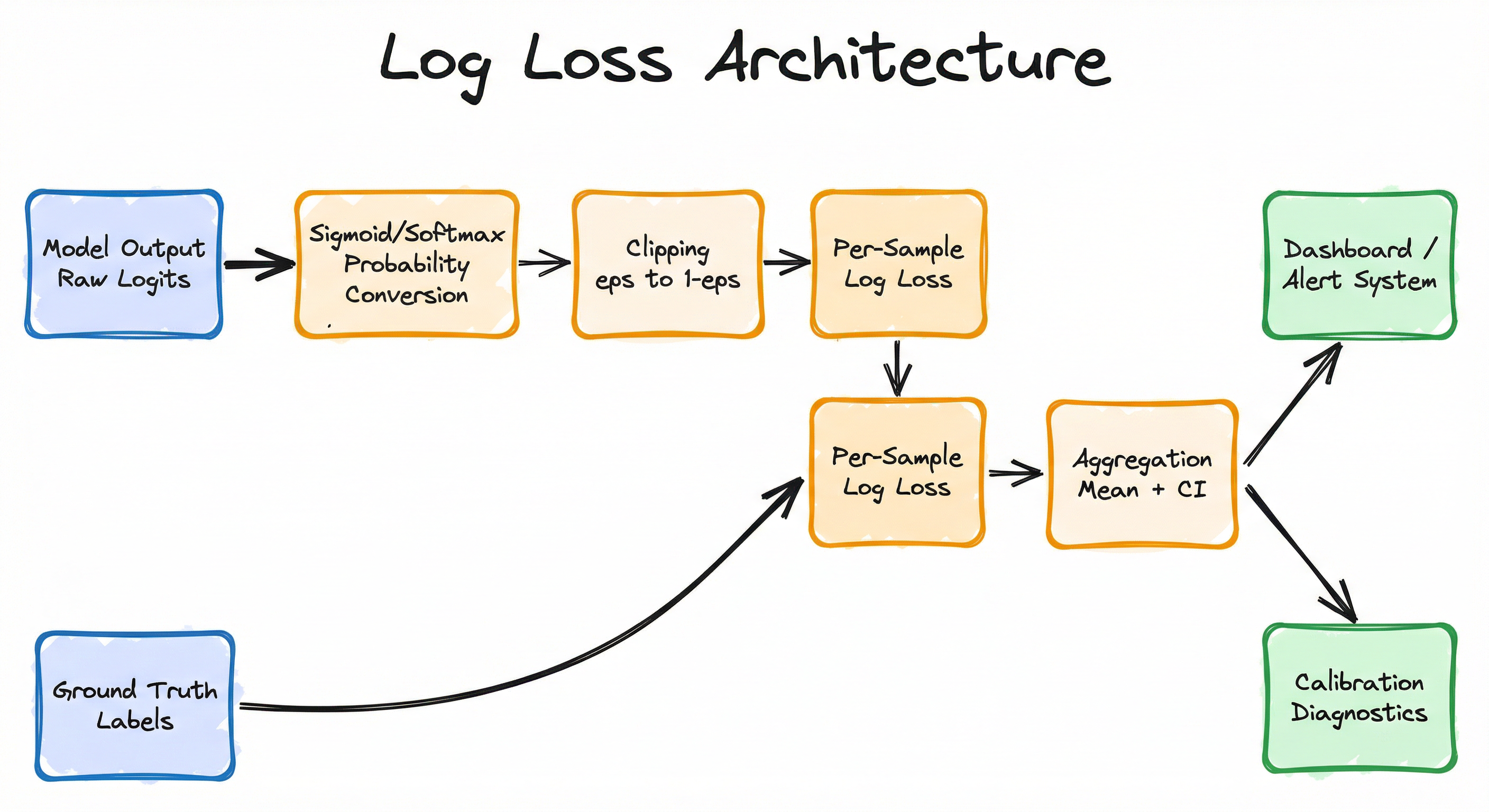
The clipping step is critical -- without it, a single prediction of exactly 0.0 or 1.0 for the wrong class sends the log loss to infinity, which corrupts the entire batch metric.
Key Components
Probability Converter
Converts raw model outputs (logits) into proper probabilities using sigmoid (binary) or softmax (multi-class). Ensures outputs are in the valid [0, 1] range and sum to 1 for multi-class problems.
Numerical Clipper
Clips predicted probabilities to the range where is typically (scikit-learn default) or (TensorFlow default). Prevents which would make the metric undefined.
Per-Sample Loss Calculator
Applies the binary cross-entropy formula or the categorical cross-entropy formula to each sample, producing a vector of individual losses.
Aggregator
Computes the mean of per-sample losses to produce the final log loss scalar. Optionally computes bootstrap confidence intervals, per-class decomposition, and class-weighted averages for imbalanced datasets.
Calibration Diagnostics
Generates calibration curves (reliability diagrams), expected calibration error (ECE), and probability histograms to assess whether the model's probability outputs match observed frequencies. Essential for interpreting what the log loss value means in context.
Data Flow
Evaluation Path: Raw model outputs (logits or probabilities) arrive alongside ground truth labels. The probability converter ensures valid probability values. The clipper applies numerical safeguards. Per-sample losses are computed and then aggregated into the final metric. Calibration diagnostics run in parallel to provide interpretability.
Training Path: During model training, the same per-sample loss computation runs in the forward pass. Gradients are computed via backpropagation, and the optimizer updates model weights to minimize the mean log loss. The clipping step is handled by the deep learning framework's numerical stability implementations (e.g., PyTorch's BCEWithLogitsLoss operates on logits directly, avoiding the need for explicit clipping).
Monitoring Path: In production, predictions are logged with timestamps. When ground truth labels become available (which can be delayed by hours or days for some applications), the log loss pipeline computes batch-level metrics and updates rolling averages in the monitoring dashboard.
A left-to-right flow from 'Model Output (Raw Logits)' through 'Sigmoid/Softmax Probability Conversion', 'Numerical Clipping', and 'Per-Sample Log Loss Computation' (which also receives Ground Truth Labels), then to 'Aggregation (Mean + Confidence Interval)', which feeds both a 'Dashboard/Alert System' and a 'Calibration Diagnostics' branch.
How to Implement
Two Contexts: Training vs. Evaluation
Log loss appears in two distinct contexts in an ML system, and the implementation details differ significantly.
As a training loss function, log loss (cross-entropy) is computed on mini-batches during forward passes, and gradients flow backward to update model parameters. Deep learning frameworks (PyTorch, TensorFlow) provide numerically stable implementations that operate on raw logits rather than probabilities, combining the sigmoid/softmax and log operations into a single numerically stable computation. This is critical -- computing sigmoid(x) followed by log(sigmoid(x)) separately can produce log(0) for extreme logits, while log_sigmoid(x) or BCEWithLogitsLoss avoids this issue.
As an evaluation metric, log loss is computed on an entire validation or test set. Libraries like scikit-learn provide log_loss() which handles multi-class problems, sample weighting, and numerical clipping. The evaluation context requires less numerical care (since probabilities are already computed) but more attention to interpretation: What does a log loss of 0.45 mean? Is it good or bad? That depends entirely on the baseline -- a random model's log loss on balanced binary classification is , so 0.45 represents meaningful improvement over random guessing.
Cost Context: Computing log loss itself is computationally trivial -- O(n) for n samples. The real cost is in generating the probability predictions that feed into it. For a deep learning model on GPU (e.g., an A100 on Azure at ~$3.40/hour or ~INR 285/hour), evaluation on a 1M-sample test set takes seconds. The compute cost is dominated by the forward pass, not the metric computation.
import numpy as np
from sklearn.metrics import log_loss

# Binary classification
y_true_binary = [1, 0, 1, 1, 0, 1, 0, 0]
y_pred_binary = [0.9, 0.1, 0.8, 0.65, 0.3, 0.95, 0.05, 0.2]

loss = log_loss(y_true_binary, y_pred_binary)
print(f"Binary log loss: {loss:.4f}")  # ~0.1897

# Compare with a worse model
y_pred_worse = [0.6, 0.4, 0.55, 0.52, 0.45, 0.6, 0.4, 0.45]
loss_worse = log_loss(y_true_binary, y_pred_worse)
print(f"Worse model log loss: {loss_worse:.4f}")  # ~0.6365

# Random baseline for binary classification
y_pred_random = [0.5] * len(y_true_binary)
loss_random = log_loss(y_true_binary, y_pred_random)
print(f"Random baseline: {loss_random:.4f}")  # ~0.6931 (= ln(2))

# Multi-class log loss (3 classes)
y_true_multi = [0, 1, 2, 0, 1, 2]
y_pred_multi = [
    [0.85, 0.10, 0.05],  # Confident correct
    [0.05, 0.90, 0.05],  # Confident correct
    [0.10, 0.20, 0.70],  # Fairly confident correct
    [0.70, 0.20, 0.10],  # Correct
    [0.30, 0.40, 0.30],  # Weakly correct
    [0.10, 0.10, 0.80],  # Confident correct
]

multi_loss = log_loss(y_true_multi, y_pred_multi)
print(f"Multi-class log loss: {multi_loss:.4f}")  # ~0.2709

# With sample weights (e.g., upweight minority class)
sample_weights = [2.0, 1.0, 1.0, 2.0, 1.0, 1.0]
weighted_loss = log_loss(y_true_multi, y_pred_multi,
                         sample_weight=sample_weights)
print(f"Weighted log loss: {weighted_loss:.4f}")
scikit-learn's log_loss handles binary and multi-class problems automatically. For binary inputs, pass a 1D array of probabilities for the positive class. For multi-class, pass an n x K matrix of probabilities (rows must sum to 1). The sample_weight parameter allows upweighting important or minority-class samples. Internally, probabilities are clipped to [eps, 1 - eps] where eps = 1e-15 to avoid numerical issues.
import torch
import torch.nn as nn

# Binary cross-entropy: ALWAYS use BCEWithLogitsLoss
# (combines sigmoid + BCE for numerical stability)
criterion_binary = nn.BCEWithLogitsLoss()

# Raw logits from model (NOT probabilities)
logits = torch.tensor([2.5, -1.0, 0.3, -3.0, 1.5])
targets = torch.tensor([1.0, 0.0, 1.0, 0.0, 1.0])

loss = criterion_binary(logits, targets)
print(f"Binary CE loss: {loss.item():.4f}")  # ~0.3159

# With class weights for imbalanced data
# E.g., positive class 5x rarer
pos_weight = torch.tensor([5.0])
criterion_weighted = nn.BCEWithLogitsLoss(pos_weight=pos_weight)
loss_weighted = criterion_weighted(logits, targets)
print(f"Weighted BCE loss: {loss_weighted:.4f}")

# Multi-class cross-entropy
criterion_multi = nn.CrossEntropyLoss()  # Expects raw logits

# Raw logits: shape (batch_size, num_classes)
logits_multi = torch.tensor([
    [2.0, 0.5, -1.0],  # Predicts class 0
    [-0.5, 3.0, 0.2],  # Predicts class 1
    [0.1, -0.3, 2.5],  # Predicts class 2
])
targets_multi = torch.tensor([0, 1, 2])  # Class indices

loss_multi = criterion_multi(logits_multi, targets_multi)
print(f"Multi-class CE loss: {loss_multi.item():.4f}")

# Label smoothing (regularization technique)
criterion_smooth = nn.CrossEntropyLoss(label_smoothing=0.1)
loss_smooth = criterion_smooth(logits_multi, targets_multi)
print(f"With label smoothing: {loss_smooth.item():.4f}")
In PyTorch, always use BCEWithLogitsLoss instead of BCELoss for binary classification. The former takes raw logits and applies the sigmoid internally using a numerically stable computation (log-sum-exp trick). Similarly, CrossEntropyLoss for multi-class takes raw logits and applies log_softmax internally. The label_smoothing parameter softens the hard 0/1 targets to [smoothing/K, 1 - smoothing + smoothing/K], which acts as a regularizer and prevents the model from becoming overconfident.
import numpy as np
from sklearn.calibration import calibration_curve
from sklearn.metrics import log_loss, brier_score_loss
import matplotlib.pyplot as plt

def evaluate_probability_quality(y_true, y_prob, n_bins=10):
    """Comprehensive probability quality assessment."""
    # Core metrics
    ll = log_loss(y_true, y_prob)
    bs = brier_score_loss(y_true, y_prob)

    # Calibration curve
    prob_true, prob_pred = calibration_curve(
        y_true, y_prob, n_bins=n_bins, strategy='uniform'
    )

    # Expected Calibration Error (ECE)
    bin_counts = np.histogram(y_prob, bins=n_bins, range=(0, 1))[0]
    bin_weights = bin_counts / len(y_prob)
    ece = np.sum(
        bin_weights[:len(prob_true)] * np.abs(prob_true - prob_pred)
    )

    # Sharpness: how spread out are the predictions?
    sharpness = np.std(y_prob)

    print(f"Log Loss:           {ll:.4f}")
    print(f"Brier Score:        {bs:.4f}")
    print(f"ECE:                {ece:.4f}")
    print(f"Sharpness (std):    {sharpness:.4f}")
    print(f"Mean prediction:    {np.mean(y_prob):.4f}")
    print(f"Actual prevalence:  {np.mean(y_true):.4f}")

    # Plot reliability diagram
    fig, (ax1, ax2) = plt.subplots(1, 2, figsize=(12, 5))

    ax1.plot([0, 1], [0, 1], 'k--', label='Perfectly calibrated')
    ax1.plot(prob_pred, prob_true, 's-', label=f'Model (ECE={ece:.3f})')
    ax1.set_xlabel('Mean predicted probability')
    ax1.set_ylabel('Fraction of positives')
    ax1.set_title('Reliability Diagram')
    ax1.legend()

    ax2.hist(y_prob, bins=n_bins, edgecolor='black', alpha=0.7)
    ax2.set_xlabel('Predicted probability')
    ax2.set_ylabel('Count')
    ax2.set_title('Prediction Distribution')

    plt.tight_layout()
    plt.savefig('calibration_diagnostics.png', dpi=150)
    return {'log_loss': ll, 'brier_score': bs, 'ece': ece}

# Example usage
np.random.seed(42)
n = 5000
y_true = np.random.binomial(1, 0.3, n)  # 30% positive rate

# Well-calibrated model
y_prob_good = np.clip(
    y_true * np.random.beta(5, 2, n) +
    (1 - y_true) * np.random.beta(2, 5, n),
    0.01, 0.99
)

results = evaluate_probability_quality(y_true, y_prob_good)
This example shows how to combine log loss with calibration diagnostics for a complete probability quality assessment. Low log loss alone does not guarantee good calibration -- a model can have low log loss because it ranks well (good discrimination) even if its probabilities are systematically off. The reliability diagram (calibration curve) reveals whether predicted probabilities match observed frequencies, while the Expected Calibration Error (ECE) quantifies calibration in a single number. In production, you want both low log loss AND low ECE.
import numpy as np
from sklearn.metrics import log_loss
from dataclasses import dataclass
from collections import deque
from datetime import datetime
from typing import Optional

@dataclass
class LogLossAlert:
    timestamp: datetime
    current_loss: float
    baseline_loss: float
    degradation_pct: float
    sample_count: int

class LogLossMonitor:
    """Rolling log loss monitor with alerting."""

    def __init__(
        self,
        baseline_loss: float,
        window_size: int = 1000,
        alert_threshold_pct: float = 10.0,
        eps: float = 1e-15,
    ):
        self.baseline = baseline_loss
        self.window_size = window_size
        self.alert_threshold = alert_threshold_pct
        self.eps = eps
        self._labels = deque(maxlen=window_size)
        self._probs = deque(maxlen=window_size)

    def add_prediction(
        self, y_true: int, y_prob: float
    ) -> Optional[LogLossAlert]:
        """Add a single prediction and check for degradation."""
        y_prob = np.clip(y_prob, self.eps, 1 - self.eps)
        self._labels.append(y_true)
        self._probs.append(y_prob)

        if len(self._labels) < 100:
            return None  # Not enough data yet

        current = log_loss(
            list(self._labels), list(self._probs)
        )
        degradation = (
            (current - self.baseline) / self.baseline * 100
        )

        if degradation > self.alert_threshold:
            return LogLossAlert(
                timestamp=datetime.now(),
                current_loss=current,
                baseline_loss=self.baseline,
                degradation_pct=degradation,
                sample_count=len(self._labels),
            )
        return None

# Usage
monitor = LogLossMonitor(
    baseline_loss=0.35,  # Established during model validation
    window_size=5000,
    alert_threshold_pct=15.0,  # Alert on 15% degradation
)

# Simulate production predictions
for y_true, y_prob in zip(true_labels, predicted_probs):
    alert = monitor.add_prediction(y_true, y_prob)
    if alert:
        print(
            f"ALERT: Log loss degraded {alert.degradation_pct:.1f}%"
            f" ({alert.baseline_loss:.4f} -> {alert.current_loss:.4f})"
        )
This production monitoring example tracks log loss over a rolling window of recent predictions. When ground truth labels become available (which can be delayed), predictions are matched and the rolling log loss is updated. If the current log loss degrades beyond a configurable threshold relative to the baseline (established during validation), an alert fires. This pattern is used at companies like PhonePe and Razorpay to detect model degradation caused by data drift, feature pipeline failures, or upstream model changes.
# Model evaluation config (YAML)
evaluation:
  primary_metric: log_loss
  metrics:
    - name: log_loss
      clip_eps: 1e-15
      sample_weight_by: inverse_class_frequency
    - name: brier_score
    - name: calibration_ece
      n_bins: 15
      strategy: uniform
  monitoring:
    baseline_log_loss: 0.35
    alert_threshold_pct: 15.0
    rolling_window: 5000
    min_samples_for_alert: 200
  calibration:
    method: isotonic  # or 'platt' (sigmoid)
    cv_folds: 5
Common Implementation Mistakes
- ●
Computing log(0): Passing a predicted probability of exactly 0.0 or 1.0 to the log function produces -infinity, corrupting the entire batch metric. Always clip predictions:
np.clip(y_prob, 1e-15, 1 - 1e-15). Better yet, usesklearn.metrics.log_losswhich handles this automatically, orBCEWithLogitsLossin PyTorch which operates on logits. - ●
Using BCELoss instead of BCEWithLogitsLoss in PyTorch:
BCELossrequires pre-computed probabilities via sigmoid, which can cause numerical instability for extreme logit values.BCEWithLogitsLosscombines sigmoid and log into a numerically stable single operation using the log-sum-exp trick. This is not optional -- it's a correctness issue. - ●
Comparing log loss across datasets with different class distributions: A log loss of 0.4 on a dataset with 50% positive rate is very different from 0.4 on a dataset with 1% positive rate. Always compare against the appropriate baseline: where is the positive class prevalence. Without this baseline, the raw number is meaningless.
- ●
Interpreting low log loss as good calibration: Log loss can be decomposed into a calibration component and a refinement (sharpness) component. A model can achieve low log loss through excellent ranking alone, even if its probabilities are systematically miscalibrated. Always complement log loss with a calibration curve and ECE.
- ●
Not accounting for sample weights in imbalanced datasets: On a dataset with 99% negative samples, log loss is dominated by the loss on negative samples. If your business objective prioritizes detecting the 1% positive cases, use sample weights to upweight them. Both
sklearn.metrics.log_lossand PyTorch losses support sample/class weighting.
When Should You Use This?
Use When
Your classifier outputs probabilities that will be used directly in downstream decisions (pricing, bidding, risk scoring, treatment assignment) -- log loss ensures these probabilities are meaningful
You need a differentiable loss function for training neural networks or logistic regression -- log loss is the standard choice for classification optimization
Model calibration matters: the predicted probability of 0.7 should correspond to ~70% actual positive rate in production
You are running a Kaggle competition or ML benchmark that specifies log loss as the evaluation metric
You want a single metric that captures both discrimination (ability to rank) and calibration (probability accuracy) in one number
You are comparing models that produce probability outputs, and you want to reward confident correct predictions more than uncertain correct ones
The downstream system uses predicted probabilities for expected value calculations (e.g., expected fraud loss = probability * transaction amount)
Avoid When
Your classifier only outputs hard labels (e.g., rule-based systems, decision trees without probability calibration) -- log loss requires probability inputs and is undefined for 0/1 predictions
You care primarily about the ranking of predictions rather than their absolute probability values -- use AUC-ROC or Average Precision instead, which are threshold-independent ranking metrics
The operating threshold is fixed and known in advance -- once you commit to a specific threshold, precision, recall, and F1 at that threshold are more actionable metrics
You need an easily interpretable metric for non-technical stakeholders -- accuracy or F1 are easier to explain than 'negative log-likelihood of 0.42'
Class probabilities are extremely skewed and you care about rare-class detection -- log loss can be dominated by the majority class unless you apply sample weighting
Your model's probability outputs are known to be miscalibrated and you cannot apply post-hoc calibration -- in this case, log loss penalizes the calibration error rather than the model's actual predictive ability
Key Tradeoffs
Log Loss vs. Accuracy: The Central Tradeoff
Accuracy is a binary metric: each prediction is either correct or incorrect, and all correct predictions contribute equally. Log loss is a continuous metric: it rewards confident correct predictions and harshly penalizes confident incorrect predictions. This means a model optimized for log loss will sometimes sacrifice accuracy to improve probability calibration.
Concrete example: on a balanced binary dataset, a model that predicts 0.51 for all positive samples and 0.49 for all negative samples achieves 100% accuracy but terrible log loss (~0.693, equivalent to random guessing). A model that predicts 0.90 for positives and 0.10 for negatives achieves the same 100% accuracy but much better log loss (~0.105). The second model is genuinely more useful because its probabilities carry information.
Log Loss vs. AUC-ROC: Calibration vs. Ranking
AUC-ROC measures the model's ability to rank positive samples higher than negative samples, regardless of the absolute probability values. A model that outputs probabilities {0.001, 0.002, 0.003} for negatives and {0.004, 0.005, 0.006} for positives has perfect AUC-ROC (1.0) despite all probabilities being near zero. Log loss would heavily penalize this model because the probabilities are far from the true 0/1 labels.
Conversely, a perfectly calibrated model that has weak discrimination (overlapping probability distributions for positive and negative classes) will have good log loss but mediocre AUC-ROC.
| Metric | Measures | Sensitive to Calibration? | Sensitive to Ranking? | Proper Scoring Rule? |
|---|---|---|---|---|
| Log Loss | Probability quality | Yes | Yes | Yes (strictly) |
| Brier Score | Probability quality | Yes | Yes | Yes (strictly) |
| AUC-ROC | Ranking quality | No | Yes | No |
| Accuracy | Threshold correctness | No | Partially | No |
Log Loss vs. Brier Score: Sensitivity to Extremes
Both are proper scoring rules, but log loss is unbounded while Brier score is bounded in [0, 1]. Log loss penalizes a confident wrong prediction (, ) with a loss of 4.6, while Brier score penalizes it with only 0.98. This makes log loss much more sensitive to catastrophic errors -- a single prediction of 0.999 for a negative sample can dominate the average log loss of the entire dataset.
In practice, this means:
- Use log loss when confident misclassifications are very costly (fraud detection, medical diagnosis)
- Use Brier score when you want a more robust, outlier-resistant metric
- Use both to get a complete picture
Cost Note: At an Indian healthcare startup processing 10,000 diagnostic predictions per day, a single overconfident misdiagnosis (predicted 0.99 healthy when actually diseased) would spike log loss dramatically. This sensitivity is a feature, not a bug -- it forces the model to be honest about uncertainty in high-stakes domains.
Alternatives & Comparisons
Accuracy measures the proportion of correct hard predictions. Log loss measures the quality of soft probability predictions. Choose accuracy when you only care about the final binary decision and all errors are equally costly. Choose log loss when probability calibration matters or when you want a metric that rewards confident correct predictions. In most modern ML systems, log loss is the more informative metric because it evaluates the full probability output.
AUC-ROC measures ranking quality -- how well the model separates positive from negative samples across all thresholds. It is insensitive to calibration: a model that outputs uniformly low probabilities but ranks correctly will have high AUC-ROC but poor log loss. Choose AUC-ROC when the operating threshold is not fixed and you want threshold-independent assessment. Choose log loss when the absolute probability values matter for downstream decisions like bidding or risk pricing.
Precision, recall, and F1 evaluate performance at a specific decision threshold and are class-specific. They are essential for understanding false positive/false negative tradeoffs, especially on imbalanced data. Log loss evaluates the entire probability distribution without requiring a threshold choice. Use precision/recall/F1 when you have a fixed threshold and need to understand class-specific error rates. Use log loss during model development and threshold-free evaluation.
Pros, Cons & Tradeoffs
Advantages
Strictly proper scoring rule: The only way to minimize expected log loss is to output the true conditional probabilities, so models cannot game the metric. This theoretical guarantee makes it uniquely trustworthy among classification metrics.
Rewards calibrated confidence: Unlike accuracy which treats all correct predictions equally, log loss rewards models that are confident when right and uncertain when unsure. A prediction of 0.95 for a true positive contributes much less loss than a prediction of 0.55.
Differentiable everywhere: Log loss is smooth and differentiable, making it an ideal training objective for gradient-based optimization. This is why cross-entropy is the standard loss function for logistic regression and neural network classifiers.
Naturally extends to multi-class: The categorical cross-entropy generalization handles any number of classes without modification. No need for one-vs-rest or binarization schemes.
Unified training and evaluation metric: Using log loss for both training and evaluation eliminates the impedance mismatch between what the model optimizes and what you measure. This simplifies model selection and hyperparameter tuning.
Information-theoretic foundation: Rooted in Shannon entropy and KL divergence, log loss has deep theoretical justification. Minimizing log loss is equivalent to maximum likelihood estimation, connecting it to a century of statistical theory.
Sensitive to catastrophic errors: The logarithmic penalty means a single overconfident wrong prediction is immediately visible in the metric. This sensitivity is valuable in high-stakes applications like medical diagnosis and fraud detection.
Disadvantages
Unbounded and hard to interpret: Log loss ranges from 0 to infinity, with no intuitive upper bound. A log loss of 0.42 does not have an obvious meaning without comparison to a baseline, unlike accuracy (0.85 = 85% correct) which is immediately interpretable.
Extremely sensitive to outlier predictions: A single prediction of 0.001 for a true positive contributes log loss of 6.9, which can dominate the average across thousands of well-calibrated predictions. This sensitivity can make log loss noisy in small samples.
Requires probability outputs: Log loss is undefined for models that only produce hard class labels (rule-based systems, some decision tree implementations). You cannot compute log loss without calibrated probability estimates.
Dominated by majority class on imbalanced data: Without sample weighting, the log loss on a 99:1 imbalanced dataset is dominated by the 99% majority class. A model that perfectly predicts the majority class but ignores the minority class can still have low log loss.
Does not directly indicate operational performance: A model with log loss of 0.35 vs. 0.38 -- which one should you deploy? Log loss does not directly translate to business metrics like revenue impact, false positive rate at a specific threshold, or customer experience. You still need threshold-specific metrics for operational decisions.
Sensitive to label noise: Mislabeled samples in the ground truth receive the full logarithmic penalty, and a few mislabeled confident predictions can significantly inflate the metric. This makes log loss unreliable when label quality is poor.
Failure Modes & Debugging
Infinite loss from unclipped probabilities
Cause
A model outputs exactly 0.0 or 1.0 probability for a sample, and the true label is the opposite class. , making the entire batch log loss undefined (NaN or infinity).
Symptoms
Log loss returns inf or NaN. During training, gradients explode and loss becomes NaN. In evaluation, the metric computation fails or returns meaningless values. This can cascade into downstream monitoring and alerting failures.
Mitigation
Always clip predicted probabilities: np.clip(y_prob, 1e-15, 1 - 1e-15). Use framework-provided numerically stable implementations: PyTorch BCEWithLogitsLoss (operates on logits, not probabilities), TensorFlow tf.keras.losses.BinaryCrossentropy(from_logits=True). In production monitoring, add a pre-computation check that flags any predictions outside [eps, 1-eps].
Miscalibration masking poor discrimination
Cause
A model is post-hoc calibrated (e.g., via Platt scaling or isotonic regression), which improves log loss by fixing calibration, but the underlying model has poor discriminative ability. The low log loss gives a false sense of quality.
Symptoms
Low log loss but poor AUC-ROC or precision-recall metrics. The model assigns correct average probabilities to groups but cannot distinguish individual positive from negative samples within those groups. Downstream decision systems make poor individual-level predictions despite good aggregate statistics.
Mitigation
Always evaluate log loss alongside discrimination metrics (AUC-ROC, Average Precision). Decompose log loss into its calibration and refinement components using Murphy decomposition. Report both pre-calibration and post-calibration log loss to understand how much improvement came from calibration vs. the underlying model.
Majority-class domination on imbalanced data
Cause
On highly imbalanced datasets (e.g., 99.5% negative in fraud detection at Razorpay or PayTM), log loss is dominated by the loss on the majority class. A model that predicts ~0.005 for every sample achieves decent log loss because 99.5% of those predictions are penalized only mildly ().
Symptoms
Model appears to have good log loss but fails to detect minority-class instances. Precision and recall for the positive class are near zero. The model has effectively learned to output the class prior probability for every sample, which is the optimal constant prediction under unweighted log loss.
Mitigation
Apply sample weighting proportional to inverse class frequency: log_loss(y_true, y_prob, sample_weight=weights). Alternatively, compute log loss separately for each class and report both. In PyTorch, use pos_weight in BCEWithLogitsLoss. In extreme cases, use stratified evaluation where you compute log loss on balanced subsamples.
Label noise amplification
Cause
Ground truth labels contain errors (mislabeled samples). When a model correctly predicts 0.95 for a true positive, but the label is incorrectly marked as 0, the per-sample log loss is -- a massive penalty for being right. Label noise disproportionately affects log loss compared to accuracy because the logarithmic penalty amplifies the impact of each mislabeled sample.
Symptoms
Log loss is higher than expected given the model's discrimination and calibration quality. The model's log loss improves significantly when evaluated on a clean subset. Confident predictions (near 0 or 1) contribute disproportionately to the total loss, and many of these correspond to mislabeled samples.
Mitigation
Apply label smoothing during training: replace hard labels 0/1 with where -. This prevents the model from becoming overconfident on potentially noisy labels. During evaluation, use robust variants like the trimmed mean (exclude top/bottom 1% of per-sample losses). Invest in label quality: at Indian startups with crowdsourced labeling pipelines, improving labeler agreement from 85% to 95% often reduces log loss more than model architecture changes.
Distribution shift causing silent degradation
Cause
The production data distribution shifts from the training distribution over time (covariate shift, concept drift). The model's probability estimates, which were well-calibrated on the training distribution, become systematically miscalibrated on the new distribution.
Symptoms
Rolling log loss gradually increases over weeks or months. Calibration curves that were previously aligned with the diagonal begin to deviate. The model's average predicted probability drifts away from the observed positive rate. This degradation is gradual and easy to miss without continuous monitoring.
Mitigation
Implement rolling log loss monitoring with a sliding window (1,000-10,000 samples). Set alerts when log loss degrades more than 10-15% from the validation baseline. Schedule periodic recalibration using recent production data. Use Platt scaling or isotonic regression on a rolling holdout set. Track the reliability diagram over time, not just the scalar log loss. At Indian fintech companies where transaction patterns shift seasonally (Diwali, end-of-quarter, etc.), build calendar-aware baselines.
Placement in an ML System
Where Does Log Loss Sit in the Pipeline?
Log loss appears at three distinct points in a typical ML system:
1. Training Loop: As the optimization objective (cross-entropy loss). Every forward pass through a neural network or gradient-boosted tree computation produces a per-batch log loss that drives parameter updates. This is the most computationally intensive use, running millions of times during training.
2. Model Selection: During hyperparameter tuning and model comparison, log loss on a validation set determines which model configuration to select. This typically runs hundreds to thousands of times during an experiment cycle. Teams at Flipkart, Swiggy, and other Indian tech companies use log loss on held-out validation data as the primary selection criterion for classifiers that produce probability outputs.
3. Production Monitoring: Once deployed, log loss is computed continuously on a rolling window of recent predictions matched with their ground truth labels. This is the least computationally expensive use but the most operationally critical -- it's how you detect model degradation, data drift, and feature pipeline failures before they impact users.
Log loss connects the model evaluation stage to the model registry (deciding which model version to promote) and to the A/B testing framework (comparing model versions in production). It is upstream of all deployment decisions and downstream of all prediction generation.
Pipeline Stage
Evaluation / Model Selection
Upstream
- Model Serving Endpoint
- Ground Truth Labels
- Feature Store
Downstream
- Model Registry
- A/B Test Runner
- Monitoring Dashboard
Scaling Bottlenecks
Log loss computation itself is O(n) and trivially parallelizable -- computing it on 100 million predictions takes seconds on a single CPU core. The bottleneck is not the metric computation but the ground truth labeling pipeline: you need labeled outcomes to compute log loss, and in many applications (fraud detection, ad click-through, loan default), the true label arrives hours, days, or months after the prediction. This delayed feedback creates a monitoring lag where your most recent log loss estimate might be days old. At scale (e.g., PhonePe processing 100M+ transactions daily), the labeling join operation itself can be expensive, requiring distributed processing with Spark or similar frameworks.
Production Case Studies
Google's ad click prediction system uses log loss (cross-entropy) as the primary training objective and evaluation metric for predicting click-through rates (CTR) on search ads. Their 2013 landmark paper "Ad Click Prediction: A View from the Trenches" describes how probability calibration is essential because predicted CTR directly determines ad auction pricing. A miscalibrated model that overestimates CTR by 10% effectively overcharges advertisers by 10%, while underestimation leaves revenue on the table.
Google's focus on log loss optimization and calibration enabled per-query calibrated bidding that generates over $200B in annual ad revenue. They demonstrated that a 0.1% improvement in log loss translates to millions of dollars in pricing accuracy, establishing log loss as the gold standard metric for CTR prediction across the industry.
Razorpay's fraud detection system uses probabilistic classifiers to score transactions with fraud probabilities. Log loss is a key evaluation metric because the fraud score feeds into a tiered decision system: low-risk transactions are auto-approved, medium-risk transactions trigger 2FA or OTP verification, and high-risk transactions are blocked. The probability value -- not just the binary fraud/not-fraud decision -- determines which tier each transaction enters.
By optimizing for log loss and calibrating their fraud models, Razorpay reduced false positive rates by over 40% while maintaining fraud catch rates. This improvement in probability quality meant fewer legitimate transactions were incorrectly flagged for review, directly improving merchant experience and reducing operational review costs estimated at INR 2-3 per reviewed transaction.
Meta's News Feed ranking system trains multi-task classifiers that predict probabilities for engagement events (click, like, comment, share, hide) on each candidate post. These probability estimates are combined into a value score using a weighted sum, and posts are ranked by this score. Meta uses normalized cross-entropy (NCE) -- a variant of log loss divided by the entropy of the background positive rate -- as the primary offline evaluation metric. NCE normalizes for class imbalance across different engagement types.
Meta's investment in log loss optimization and calibration for their ranking models serves 2+ billion daily active users. Their engineering blog reports that improvements in NCE (normalized log loss) correlate directly with improvements in user engagement metrics. A 1% improvement in NCE for the engagement prediction model was shown to translate into measurable improvements in session time and user satisfaction.
Google Developers Machine Learning Crash Course explains log loss as the loss function for logistic regression, using the formula LogLoss = Σ -y × log(y') - (1-y) × log(1 - y') where y is the true label and y' is the predicted probability.
Log loss penalizes incorrect predictions more heavily than squared loss, making it particularly effective for classification problems where probability estimates are important, and has become the standard loss function for binary classification tasks.
Tooling & Ecosystem
The standard Python implementation for evaluating log loss. Handles binary and multi-class problems, supports sample weights, and clips probabilities to avoid numerical issues. The go-to choice for evaluation. Also includes sklearn.calibration.CalibratedClassifierCV for post-hoc calibration and calibration_curve for reliability diagrams.
Numerically stable implementations for training. BCEWithLogitsLoss for binary, CrossEntropyLoss for multi-class. Both accept raw logits and handle sigmoid/softmax internally. Support class weighting (pos_weight, weight), label smoothing, and reduction strategies (mean, sum, none).
Keras loss classes for training neural networks. Support from_logits=True for numerical stability and label_smoothing for regularization. Integrated with Keras metrics API for computing running log loss during training and evaluation callbacks.
Both gradient boosting frameworks use log loss (binary/multi-class logistic) as the default objective for classification. XGBoost uses binary:logistic and multi:softprob; LightGBM uses binary and multiclass. Both provide logloss as a built-in evaluation metric for early stopping during training.
A comprehensive calibration library that provides temperature scaling, Platt scaling, isotonic regression, beta calibration, and other post-hoc calibration methods. Essential for improving log loss without retraining the model. Also includes ECE computation and reliability diagram generation.
Experiment tracking platform that logs log loss values across training runs, enabling comparison of models and hyperparameter configurations. Supports automatic logging from scikit-learn, PyTorch, and TensorFlow. Widely used at Indian startups and enterprises for ML experiment management.
Research & References
Shannon, C. E. (1948)Bell System Technical Journal
The foundational paper that introduced entropy, cross-entropy, and the information-theoretic framework underlying log loss. Shannon proved that is the optimal encoding length for an event with probability , which is the direct theoretical basis for why log loss measures prediction quality.
Gneiting, T. and Raftery, A. E. (2007)Journal of the American Statistical Association
The definitive mathematical treatment of proper scoring rules, proving that log loss (logarithmic score) and Brier score are strictly proper scoring rules. Establishes the theoretical foundation for why these metrics encourage honest probabilistic predictions and cannot be gamed.
McMahan, H. B. et al. (2013)KDD 2013
Google's seminal paper on large-scale click prediction using FTRL-Proximal optimization with log loss as the primary objective and evaluation metric. Demonstrated the critical importance of probability calibration for ad pricing and introduced normalized entropy as a calibration-aware variant of log loss.
Naeini, M. P., Cooper, G. F., and Hauskrecht, M. (2015)AAAI 2015
Introduced the Bayesian Binning into Quantiles (BBQ) calibration method and formalized Expected Calibration Error (ECE) as a companion metric to log loss. Showed that post-hoc calibration consistently improves log loss across various classifier types.
Guo, C., Pleiss, G., Sun, Y., and Weinberger, K. Q. (2017)ICML 2017
Demonstrated that modern deep neural networks are significantly miscalibrated despite having low training cross-entropy loss. Introduced temperature scaling -- a single-parameter post-hoc calibration method that consistently improves log loss on held-out data. This paper is essential reading for anyone deploying neural classifiers.
Interview & Evaluation Perspective
Common Interview Questions
- ●
What is log loss and why is it preferred over accuracy for evaluating probabilistic classifiers?
- ●
Explain the relationship between log loss, cross-entropy, negative log-likelihood, and KL divergence.
- ●
How does log loss handle multi-class classification? Walk me through the formula.
- ●
What does it mean that log loss is a strictly proper scoring rule? Why does this matter?
- ●
Compare log loss with Brier score. When would you prefer one over the other?
- ●
A model has excellent AUC-ROC (0.95) but poor log loss (1.2). How is this possible and what would you do?
- ●
How would you detect and fix a calibration problem using log loss and calibration curves?
- ●
Design a monitoring system for log loss in production. What alerts would you set?
Key Points to Mention
- ●
Log loss is the negative average log-probability assigned to the true class -- it measures how well the model's confidence matches reality. Always state the formula clearly: .
- ●
It is a strictly proper scoring rule, meaning the only way to minimize expected log loss is to output the true conditional probabilities. This is the key theoretical advantage over accuracy and F1.
- ●
Minimizing log loss is equivalent to maximum likelihood estimation -- training logistic regression and neural networks with cross-entropy loss IS log loss minimization.
- ●
Log loss decomposes into calibration + refinement (Murphy decomposition). A model can have low log loss from either excellent calibration or excellent discrimination or both.
- ●
The baseline for binary log loss is (random guessing on balanced data). Always compare against the appropriate baseline: where is the positive prevalence.
- ●
In production systems, log loss matters because downstream systems (pricing, bidding, risk scoring) consume probability values, not just binary decisions. Miscalibrated probabilities lead to mispriced risk.
Pitfalls to Avoid
- ●
Stating that log loss ranges from 0 to 1 -- it's unbounded above (ranges from 0 to infinity). The Brier score ranges from 0 to 1, and confusing them is a common interview mistake.
- ●
Forgetting numerical stability: never discuss log loss without mentioning the need to clip probabilities or use logit-space implementations. This shows production awareness.
- ●
Claiming that low log loss implies good calibration -- it's a necessary but not sufficient condition. A model with excellent ranking but poor calibration can have lower log loss than you'd expect.
- ●
Ignoring class imbalance: unweighted log loss on a 99:1 dataset is dominated by the majority class. Always mention sample weighting when discussing imbalanced scenarios.
- ●
Not distinguishing log loss as a training objective vs. an evaluation metric -- interviewers expect you to understand both roles and why using the same metric for both is advantageous.
Senior-Level Expectation
A senior or staff-level candidate should discuss the full picture: the information-theoretic foundation (cross-entropy as KL divergence plus entropy), why properness matters for incentive compatibility, the decomposition of log loss into calibration and refinement components, practical calibration techniques (temperature scaling, Platt scaling, isotonic regression) with their tradeoffs, normalized entropy for fair comparison across datasets with different class distributions, the relationship between log loss optimization and maximum likelihood estimation, and production monitoring strategies including delayed-label scenarios (common at Indian fintech companies where fraud labels arrive days after the transaction). The ability to reason about when log loss is the wrong metric -- such as when the operating threshold is fixed and precision/recall at that threshold matter more -- is what separates senior engineers from mid-level. Extra credit for discussing label smoothing as a regularization technique and its effect on log loss during training vs. evaluation.
Summary
Log loss (binary cross-entropy / negative log-likelihood) is the fundamental metric for evaluating classifiers that produce probability estimates rather than just hard labels. It measures the average negative log-probability assigned to the true class labels, penalizing confident wrong predictions with unbounded logarithmic severity and rewarding confident correct predictions.
The metric's strength lies in its theoretical foundations: it is a strictly proper scoring rule (the unique optimal strategy is to output true probabilities), equivalent to maximum likelihood estimation (so it bridges training and evaluation seamlessly), and grounded in information theory (minimizing log loss equals minimizing KL divergence from the true distribution). These properties make it the default training objective for logistic regression, neural networks, and gradient boosted trees, and the primary evaluation metric for probabilistic classification systems at companies like Google (ad CTR prediction), Meta (engagement prediction), Razorpay (fraud scoring), and PhonePe (transaction risk).
In practice, log loss must be interpreted carefully: it is unbounded and hard to interpret without baselines, sensitive to outlier predictions and label noise, and dominated by the majority class on imbalanced data. The best practice is to report log loss alongside complementary metrics -- AUC-ROC for ranking quality, calibration curves and ECE for calibration quality, and precision/recall for threshold-specific performance. Post-hoc calibration techniques (temperature scaling, Platt scaling, isotonic regression) can improve log loss without retraining the model. For production monitoring, track rolling log loss with alerting on degradation relative to the validation baseline, and always account for the delayed ground truth labels that are common in applications like fraud detection and credit scoring.