MAP in Machine Learning
Here is a question that keeps coming up in every ML system design interview involving search or recommendations: you have a ranked list of results, some relevant and some not -- how do you measure whether the ranking is any good?
You could compute precision at some cutoff K, but that throws away information about where the relevant items sit within the top K. You could look at recall, but that ignores ranking entirely. You need a metric that captures both how many relevant items you retrieved and how high you ranked them.
Mean Average Precision (MAP) is exactly that metric. It has been the gold standard in information retrieval evaluation since the early TREC conferences in the 1990s, and it remains one of the most widely reported metrics in academic IR benchmarks, recommendation system evaluations, and search quality measurement.
MAP works by computing Average Precision (AP) for each query -- which summarizes the entire precision-recall curve into a single number -- and then averaging AP across all queries. The result is a value between 0 and 1 that rewards systems which place relevant documents at the top of the ranked list. A MAP of 1.0 means every relevant document appears before every irrelevant one, for every query.
From TREC's ad-hoc retrieval tracks to modern dense retrieval benchmarks like BEIR, from Flipkart's product search to JioSaavn's music recommendations -- if you are evaluating a retrieval system with binary relevance labels, MAP is likely the metric you should reach for first.
Concept Snapshot
- What It Is
- A ranking evaluation metric that averages the precision values computed at each position where a relevant document is retrieved, then averages that score across multiple queries to measure overall retrieval quality with binary relevance.
- Category
- Evaluation
- Complexity
- Intermediate
- Inputs / Outputs
- Inputs: a ranked list of retrieved items and binary relevance labels (relevant=1, not relevant=0) for each item. Outputs: a single score between 0 and 1, where 1 represents perfect retrieval ordering.
- System Placement
- Used in offline evaluation during model development, online A/B testing of ranking algorithms, and as a standard reporting metric in academic IR benchmarks (TREC, BEIR, MS MARCO).
- Also Known As
- mAP, Mean AP, MAP@K, Mean Average Precision at K
- Typical Users
- ML engineers, search engineers, IR researchers, recommendation system developers, NLP engineers working on retrieval
- Prerequisites
- Precision and recall fundamentals, Ranked retrieval concepts, Binary relevance judgments, Basic probability and averaging
- Key Terms
- Average Precision (AP)precision at rank krecallbinary relevanceinterpolated precisionnon-interpolated APMAP@Kprecision-recall curve
Why This Concept Exists
The Problem with Single-Point Metrics
Early information retrieval systems were evaluated with precision and recall -- two metrics that answer fundamentally different questions. Precision asks: "Of the items I retrieved, how many are relevant?" Recall asks: "Of all the relevant items, how many did I retrieve?"
The problem is that these metrics conflict. You can trivially achieve perfect recall by returning every document in the collection (precision drops to near zero). You can achieve perfect precision by returning only the single most confident result (recall drops to near zero). Researchers needed a way to capture the tradeoff between precision and recall across the entire ranked list.
The Precision-Recall Curve and Its Limitations
The precision-recall (PR) curve plots precision against recall at every rank position. It captures the full picture: how precision degrades as you retrieve more documents and recall increases. But a curve is not a number. You cannot say "System A is better than System B" by looking at two crossing curves. You need a single scalar that summarizes the curve.
The Birth of Average Precision
The solution emerged from the TREC (Text REtrieval Conference) community in the early 1990s. TREC, organized by NIST (National Institute of Standards and Technology) and led by Donna Harman and Ellen Voorhees, needed a standard metric to compare dozens of retrieval systems submitted by research groups worldwide.
Average Precision (AP) was the answer: it computes the area under the precision-recall curve (approximately) by averaging precision at every position where a relevant document is retrieved. This single number captures both precision and recall -- it rewards systems that retrieve relevant documents early and penalizes those that bury relevant documents deep in the list.
Mean Average Precision (MAP) is simply the mean of AP across all queries in the evaluation set. This handles the fact that different queries have different numbers of relevant documents and different difficulty levels. By averaging AP across queries, MAP provides a stable, robust measure of overall system quality.
Why MAP Became the Standard
Buckley and Voorhees (2004) showed that MAP has especially good discrimination (it can distinguish between systems with small quality differences) and stability (rankings of systems are consistent across different query sets). These properties made MAP the default metric in TREC evaluations for over two decades.
Key Insight: MAP exists because we need a single number that captures the full precision-recall tradeoff across a ranked list, averaged across queries of varying difficulty. It is the natural summary of the precision-recall curve, and its statistical properties make it ideal for comparing retrieval systems.
Core Intuition & Mental Model
The Elevator Pitch
Imagine you are a librarian helping patrons find books. For each request (query), you pull books off the shelves and stack them in a pile, with your best guesses on top.
MAP measures how good you are at this job across many patrons. Specifically, every time you place a relevant book in the stack, it checks: "What fraction of the books above this one (inclusive) are relevant?" Then it averages those fractions. If all the relevant books are at the very top of every stack, you get a perfect score of 1.0.
Walking Through AP Step by Step
Let's say a user searches for "machine learning tutorials" and there are 4 relevant documents in the collection. Your system returns 10 results:
Position: [1, 2, 3, 4, 5, 6, 7, 8, 9, 10] Relevant?: [1, 0, 1, 0, 0, 1, 0, 0, 0, 1]
Now, compute precision at each position where a relevant document appears:
- Position 1: Precision = 1/1 = 1.00 (1 relevant out of 1 seen)
- Position 3: Precision = 2/3 = 0.67 (2 relevant out of 3 seen)
- Position 6: Precision = 3/6 = 0.50 (3 relevant out of 6 seen)
- Position 10: Precision = 4/10 = 0.40 (4 relevant out of 10 seen)
Average Precision = (1.00 + 0.67 + 0.50 + 0.40) / 4 = 0.64
Notice what happens: the first relevant document (position 1) contributes a full 1.00 to the average, but the last one (position 10) only contributes 0.40. Relevant documents ranked higher contribute more to AP. This is why MAP rewards systems that put relevant items first.
Why "Average" Appears Twice
The name "Mean Average Precision" sounds redundant, but the two averages operate at different levels:
- Average Precision (AP): averages precision values within a single query (across relevant document positions)
- Mean AP: averages AP values across multiple queries
This two-level averaging is what makes MAP robust: AP handles within-query variation (different numbers of relevant documents), and the mean handles across-query variation (different query difficulties).
The Area-Under-the-Curve Connection
Here is an elegant way to think about AP: it approximates the area under the precision-recall curve. Each relevant document you find increases recall by (where is the total number of relevant documents), and the precision at that point is the "height" of the curve. Summing precision recall-increment gives you the area. This is why AP is sometimes called "area under the PR curve" -- the approximation is exact for non-interpolated AP.
Mental Model: Think of AP as a grade on a scavenger hunt. Finding treasures early earns you high marks. Finding them late earns low marks. Missing them entirely earns zero. MAP is your grade averaged across many scavenger hunts.
Technical Foundations
Building MAP From First Principles
Let's formalize MAP step by step, building from precision through AP to MAP.
Step 1: Precision at Rank
For a query , given a ranked list of retrieved documents , precision at rank is:
Or equivalently:
where is the binary relevance label of document .
Step 2: Average Precision (AP)
Average Precision for a single query with total relevant documents:
Breaking this down:
- The sum iterates over all positions in the ranked list
- acts as a selector: we only compute precision at positions where a relevant document appears
- is the precision at that position
- We divide by (total relevant documents, including those not retrieved) to penalize missed relevant documents
Critical detail: The denominator is (total relevant documents in the collection), not the number of relevant documents actually retrieved. If your system retrieves only 3 of 10 relevant documents, the denominator is 10. The 7 unretreived relevant documents implicitly contribute precision of 0, dragging AP down. This is how MAP penalizes low recall.
Step 3: MAP (Mean Average Precision)
Given a set of queries :
Simply the arithmetic mean of AP across all queries.
Step 4: MAP@K (MAP at Cutoff K)
In practice, we often evaluate only the top results:
Note: Some implementations use (total relevant docs) as the denominator even for AP@K, while others use . The TREC convention uses , which means AP@K is always AP for the full list. Be explicit about which convention your implementation follows.
Worked Example
Suppose we have 2 queries, each with 5 relevant documents in the collection.
Query 1: returns [R, N, R, R, N, N, R, N, N, N] (R=relevant, N=not relevant)
- Position 1: P(1) = 1/1 = 1.00
- Position 3: P(3) = 2/3 = 0.667
- Position 4: P(4) = 3/4 = 0.75
- Position 7: P(7) = 4/7 = 0.571
- Only 4 of 5 relevant docs retrieved, so 5th contributes 0
- AP = (1.00 + 0.667 + 0.75 + 0.571 + 0) / 5 = 0.598
Query 2: returns [R, R, R, R, R, N, N, N, N, N]
- Position 1: P(1) = 1.00
- Position 2: P(2) = 1.00
- Position 3: P(3) = 1.00
- Position 4: P(4) = 1.00
- Position 5: P(5) = 1.00
- All 5 relevant docs retrieved at top 5
- AP = (1.00 + 1.00 + 1.00 + 1.00 + 1.00) / 5 = 1.00
MAP = (0.598 + 1.00) / 2 = 0.799
Interpolated vs Non-Interpolated AP
There are two variants of Average Precision, and the distinction matters:
Non-interpolated AP (TREC standard): Compute precision exactly at each position where a relevant document is found. This is what we defined above and what trec_eval computes. It is the standard in modern IR evaluation.
Interpolated AP (11-point): Compute precision at 11 fixed recall levels (0.0, 0.1, 0.2, ..., 1.0), where the interpolated precision at recall level is:
The interpolated precision at each recall level is the maximum precision found at any recall level greater than or equal to the current one. This smooths out the "zigzag" in the PR curve. The 11-point interpolated AP was used in early TREC evaluations but has largely been replaced by non-interpolated AP because interpolation can overestimate precision.
Implementation Note: Always use non-interpolated AP unless you are explicitly reproducing results from a paper that uses 11-point interpolation. Modern tools like
trec_eval,pytrec_eval, andranxdefault to non-interpolated AP.
Internal Architecture
MAP is a metric, not a deployable system component. But there is a well-defined computational pipeline for how MAP is calculated and integrated into ML evaluation workflows. Here is the architecture of a MAP evaluation pipeline.
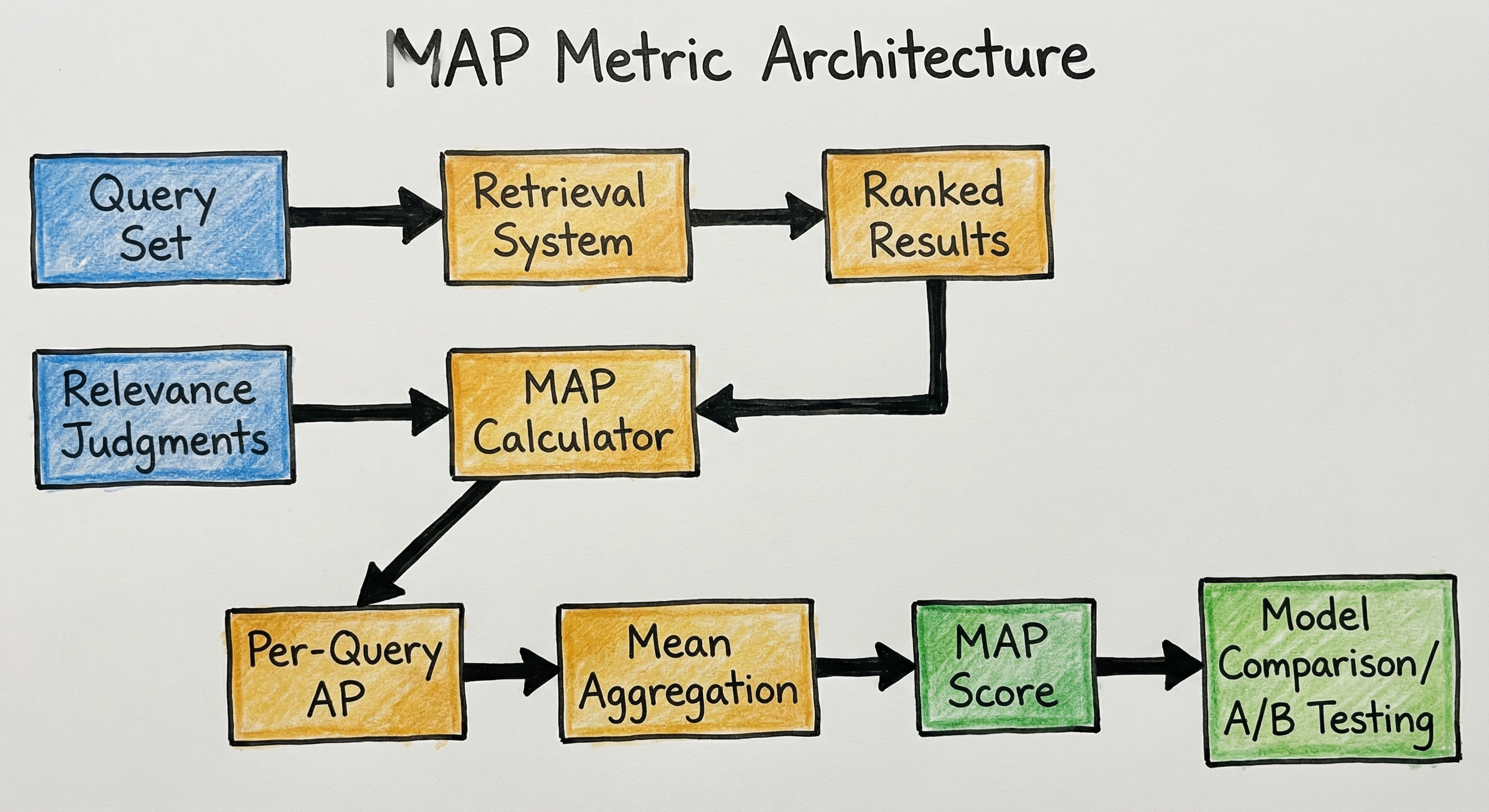
The pipeline operates in two phases. First, the retrieval system produces ranked results for each query. Second, the MAP calculator matches these results against ground-truth relevance judgments, computes AP per query, and aggregates to produce the final MAP score. This architecture is identical whether you are evaluating a sparse retriever (BM25), a dense retriever (DPR, ColBERT), or a learned re-ranker.
Key Components
Query Set
A collection of evaluation queries (typically 50-1000 queries for TREC-style benchmarks). Each query has a known set of relevant documents in the collection. The query set should represent the distribution of real user queries.
Retrieval System
The system under evaluation. Could be BM25, a neural dense retriever (DPR, ColBERT), a re-ranker, or any pipeline that produces a ranked list of documents for each query. MAP is agnostic to the retrieval method.
Relevance Judgments (qrels)
Ground-truth binary relevance labels for query-document pairs. In TREC format, these are stored as 'qrels' files: (query_id, iteration, doc_id, relevance). Relevance is binary: 0 (not relevant) or 1 (relevant). Documents not in the qrels file are assumed irrelevant.
Per-Query AP Calculator
For each query, walks down the ranked list, computes precision at every position where a relevant document appears, and averages these precision values divided by the total number of relevant documents for that query.
Mean Aggregation
Computes the arithmetic mean of AP values across all queries. This is the final MAP score. May also compute confidence intervals via bootstrapping for statistical significance testing.
Model Comparison Layer
Uses MAP scores (and statistical tests like paired t-test or bootstrap test) to determine whether one retrieval system is significantly better than another. Feeds into A/B testing decisions and model selection.
Data Flow
Here is the data flow for a standard offline evaluation:
Input: A test collection consisting of (1) a document corpus, (2) a set of queries , and (3) relevance judgments (qrels) mapping each query to its set of relevant documents.
For each query :
- The retrieval system returns a ranked list sorted by descending relevance score
- For each position in , look up whether is relevant according to qrels
- Compute at each position where
- Compute where is the total number of relevant documents for query
Output:
For online evaluation (A/B testing), the flow is similar but relevance judgments come from user behavior (clicks, purchases, engagement) rather than human annotations, and MAP is computed over cohorts of live traffic.
A directed flow diagram showing 'Query Set' and 'Relevance Judgments' as two inputs feeding into a 'MAP Calculator' that also receives 'Ranked Results' from the 'Retrieval System'. The calculator flows through 'Per-Query AP' to 'Mean Aggregation' to produce a 'MAP Score' that feeds 'Model Comparison / A/B Testing'.
How to Implement
Three Approaches to Computing MAP
There are three common ways to compute MAP in practice, each suited to different contexts:
Option A: Use ranx or ir_measures -- purpose-built IR evaluation libraries that handle TREC-format qrels, support MAP and dozens of other metrics, and are optimized with Numba for speed. Best for IR research and benchmarking.
Option B: Use scikit-learn's average_precision_score -- works for binary classification contexts where you compute AP from prediction scores and binary labels. Not designed for ranked retrieval but can be adapted. Best for quick prototyping.
Option C: Implement from scratch -- necessary when you need full control, custom cutoffs, or integration with proprietary evaluation pipelines. The formula is simple enough that a from-scratch implementation is practical and recommended for understanding.
For production evaluation pipelines, Option A is strongly recommended. For ML system design interviews, Option C demonstrates understanding. Let's walk through all three.
Cost Note: Computing MAP is computationally trivial (linear in the number of retrieved documents per query). The real cost is relevance judgment collection. For binary labels, expect INR 30-80 per query-document pair using crowdsourcing platforms. For 500 queries with 50 judged documents each = 25,000 labels, budget INR 7.5-20 lakh including quality control. Binary labels are cheaper than graded (0-4) labels because annotators only make a yes/no decision.
import numpy as np
from typing import List, Dict, Tuple

def average_precision(ranked_list: List[int], num_relevant: int) -> float:
    """Compute Average Precision for a single query.

    Args:
        ranked_list: Binary relevance labels in ranked order.
                     e.g., [1, 0, 1, 0, 0, 1] means relevant at positions 1, 3, 6.
        num_relevant: Total number of relevant documents for this query
                      (including those NOT retrieved).

    Returns:
        AP score between 0 and 1.
    """
    if num_relevant == 0:
        return 0.0

    cumulative_relevant = 0
    precision_sum = 0.0

    for k, is_relevant in enumerate(ranked_list, start=1):
        if is_relevant:
            cumulative_relevant += 1
            precision_at_k = cumulative_relevant / k
            precision_sum += precision_at_k

    return precision_sum / num_relevant


def mean_average_precision(
    queries: Dict[str, Tuple[List[int], int]]
) -> float:
    """Compute MAP across multiple queries.

    Args:
        queries: Dict mapping query_id to (ranked_list, num_relevant).

    Returns:
        MAP score between 0 and 1.
    """
    if not queries:
        return 0.0

    ap_scores = []
    for query_id, (ranked_list, num_relevant) in queries.items():
        ap = average_precision(ranked_list, num_relevant)
        ap_scores.append(ap)
        print(f"Query {query_id}: AP = {ap:.4f}")

    map_score = np.mean(ap_scores)
    print(f"\nMAP = {map_score:.4f}")
    return map_score


def average_precision_at_k(
    ranked_list: List[int], num_relevant: int, k: int
) -> float:
    """Compute AP@K (Average Precision at cutoff K).

    Only considers the top K results.
    Uses min(num_relevant, K) as denominator (common convention).
    """
    if num_relevant == 0 or k == 0:
        return 0.0

    ranked_list = ranked_list[:k]
    cumulative_relevant = 0
    precision_sum = 0.0

    for i, is_relevant in enumerate(ranked_list, start=1):
        if is_relevant:
            cumulative_relevant += 1
            precision_at_i = cumulative_relevant / i
            precision_sum += precision_at_i

    # TREC convention: divide by num_relevant (penalizes low recall)
    # Alternative: divide by min(num_relevant, k)
    return precision_sum / num_relevant


# --- Example Usage ---
queries = {
    "q1": ([1, 0, 1, 1, 0, 0, 1, 0, 0, 0], 5),  # 4 of 5 relevant found
    "q2": ([1, 1, 1, 1, 1, 0, 0, 0, 0, 0], 5),  # 5 of 5 found (perfect)
    "q3": ([0, 0, 0, 1, 0, 1, 0, 0, 1, 0], 3),  # 3 of 3 found (late)
}

map_score = mean_average_precision(queries)
# Output:
# Query q1: AP = 0.6533
# Query q2: AP = 1.0000
# Query q3: AP = 0.4278
# MAP = 0.6937
This implementation follows the standard non-interpolated AP formula used by TREC. The key design decision is the denominator: we use num_relevant (total relevant documents in the collection for this query), not just the count of relevant documents retrieved. This means if your system misses relevant documents, AP is penalized -- it implicitly captures recall. The average_precision_at_k variant only considers the top K results, useful when you only care about the first page of search results.
from ranx import Qrels, Run, evaluate

# Define ground truth relevance judgments (qrels)
# Format: {query_id: {doc_id: relevance_score}}
qrels_dict = {
    "q1": {"doc_a": 1, "doc_b": 0, "doc_c": 1, "doc_d": 1, "doc_e": 0},
    "q2": {"doc_f": 1, "doc_g": 1, "doc_h": 0, "doc_i": 1, "doc_j": 0},
    "q3": {"doc_k": 0, "doc_l": 1, "doc_m": 1, "doc_n": 0, "doc_o": 1},
}
qrels = Qrels(qrels_dict)

# Define system results (run)
# Format: {query_id: {doc_id: retrieval_score}}
# Higher score = ranked higher
run_dict = {
    "q1": {"doc_a": 0.95, "doc_c": 0.80, "doc_d": 0.70, "doc_b": 0.50, "doc_e": 0.30},
    "q2": {"doc_f": 0.90, "doc_g": 0.85, "doc_i": 0.75, "doc_h": 0.60, "doc_j": 0.40},
    "q3": {"doc_l": 0.88, "doc_o": 0.82, "doc_m": 0.70, "doc_k": 0.55, "doc_n": 0.35},
}
run = Run(run_dict)

# Compute MAP and MAP@K
results = evaluate(
    qrels,
    run,
    metrics=["map", "map@5", "map@10", "mrr", "ndcg@10"]
)

print("MAP:", results["map"])
print("MAP@5:", results["map@5"])
print("MAP@10:", results["map@10"])
print("MRR:", results["mrr"])
print("NDCG@10:", results["ndcg@10"])

# Compare two systems with statistical testing
from ranx import compare

run_bm25 = Run(run_dict, name="BM25")
run_neural = Run(run_dict, name="NeuralRetriever")  # different scores

report = compare(
    qrels=qrels,
    runs=[run_bm25, run_neural],
    metrics=["map@100", "ndcg@10", "mrr@10"],
    stat_test="paired_t",
)
print(report)
The ranx library is purpose-built for IR evaluation. It handles TREC-format qrels natively, computes MAP and 20+ other metrics efficiently (using Numba JIT compilation), and includes statistical significance testing (paired t-test, bootstrap test, Fisher randomization) out of the box. The compare function generates a formatted report showing which system is significantly better. This is the recommended approach for production evaluation pipelines.
import pytrec_eval
import json

# Qrels in TREC format: {query_id: {doc_id: relevance}}
qrels = {
    "q1": {"d1": 1, "d2": 0, "d3": 1, "d4": 1, "d5": 0, "d6": 1, "d7": 0},
    "q2": {"d8": 1, "d9": 1, "d10": 0, "d11": 1, "d12": 0, "d13": 0, "d14": 1},
}

# Run in TREC format: {query_id: {doc_id: score}}
run = {
    "q1": {"d1": 5.0, "d3": 4.5, "d2": 4.0, "d4": 3.5, "d5": 3.0, "d6": 2.5, "d7": 2.0},
    "q2": {"d8": 5.0, "d9": 4.8, "d11": 4.5, "d14": 4.0, "d10": 3.5, "d12": 3.0, "d13": 2.5},
}

# Create evaluator with desired metrics
evaluator = pytrec_eval.RelevanceEvaluator(
    qrels,
    {"map", "map_cut_5", "map_cut_10", "P_5", "recall_10", "ndcg_cut_10"}
)

# Evaluate
results = evaluator.evaluate(run)

# Print per-query results
for query_id, metrics in sorted(results.items()):
    print(f"\n{query_id}:")
    print(f"  MAP: {metrics['map']:.4f}")
    print(f"  MAP@5: {metrics['map_cut_5']:.4f}")
    print(f"  MAP@10: {metrics['map_cut_10']:.4f}")
    print(f"  P@5: {metrics['P_5']:.4f}")
    print(f"  Recall@10: {metrics['recall_10']:.4f}")
    print(f"  NDCG@10: {metrics['ndcg_cut_10']:.4f}")

# Compute mean across queries
import numpy as np
for metric in ["map", "map_cut_5", "map_cut_10"]:
    values = [results[q][metric] for q in results]
    print(f"\nMean {metric}: {np.mean(values):.4f}")
pytrec_eval is a Python wrapper around the official TREC evaluation tool (trec_eval). It produces identical results to the C implementation used by TREC organizers, making it the gold standard for reproducible evaluation. The metric names follow TREC conventions: map is non-interpolated MAP, map_cut_5 is MAP@5, P_5 is Precision@5. Use this when you need exact compatibility with TREC evaluation.
from sklearn.metrics import average_precision_score
import numpy as np

# In sklearn, AP is computed from prediction scores and binary labels
# This is for binary classification, not ranked retrieval
# But it's equivalent when you have one query

# Ground truth: binary relevance labels
y_true = np.array([1, 0, 1, 1, 0, 0, 1, 0, 0, 0])

# Predicted scores: higher = more likely relevant
y_scores = np.array([0.95, 0.80, 0.78, 0.70, 0.55, 0.40, 0.35, 0.25, 0.15, 0.05])

# Compute AP (area under the precision-recall curve)
ap = average_precision_score(y_true, y_scores)
print(f"Average Precision: {ap:.4f}")
# Output: Average Precision: 0.8393

# For MAP across multiple queries, compute AP per query and average
def compute_map_sklearn(queries):
    """Compute MAP using sklearn.

    Args:
        queries: list of (y_true, y_scores) tuples, one per query.
    """
    ap_scores = []
    for y_true, y_scores in queries:
        ap = average_precision_score(y_true, y_scores)
        ap_scores.append(ap)
    return np.mean(ap_scores)

queries = [
    (np.array([1, 0, 1, 1, 0]), np.array([0.9, 0.8, 0.7, 0.6, 0.5])),
    (np.array([1, 1, 0, 0, 1]), np.array([0.95, 0.85, 0.75, 0.3, 0.2])),
]

map_score = compute_map_sklearn(queries)
print(f"MAP: {map_score:.4f}")

# NOTE: sklearn's AP uses a slightly different formula than trec_eval
# sklearn uses trapezoidal approximation of the PR curve area
# trec_eval uses the sum-of-precisions formula
# Results differ slightly -- use pytrec_eval for TREC-compatible MAP
Scikit-learn's average_precision_score computes the area under the precision-recall curve using trapezoidal integration. This is slightly different from the TREC-standard AP formula (sum of precisions at relevant positions divided by total relevant documents). For most practical purposes the difference is small, but if you need exact TREC compatibility, use pytrec_eval or ranx instead. Sklearn's version is convenient for quick prototyping but is not designed for multi-query retrieval evaluation.
# Example: pytrec_eval metrics configuration
# Standard TREC evaluation metrics set
metrics:
  primary:
    - map                # Non-interpolated MAP (full list)
    - map_cut_10         # MAP@10
    - map_cut_100        # MAP@100
  secondary:
    - P_5                # Precision@5
    - P_10               # Precision@10
    - recall_100         # Recall@100
    - ndcg_cut_10        # NDCG@10 (for comparison)
    - recip_rank         # MRR (for comparison)

# Statistical significance testing
significance:
  test: paired_t         # or bootstrap, fisher_randomization
  alpha: 0.05
  correction: bonferroni # for multiple comparisons

# Evaluation parameters
evaluation:
  qrels_format: trec     # TREC qrels format
  depth: 1000            # Evaluate top 1000 results
  relevance_threshold: 1 # Binary: >= 1 is relevant
Common Implementation Mistakes
- ●
Using the wrong denominator in AP: The denominator should be the total number of relevant documents for the query (including those not retrieved), not just the count of relevant documents in the returned list. Using the wrong denominator inflates AP for systems with low recall.
- ●
Confusing MAP with mAP in object detection: In computer vision, mAP (mean Average Precision) uses IoU-based matching with precision-recall curves over confidence thresholds. In information retrieval, MAP uses rank-based precision over binary relevance. Same name, different computation. Be explicit about which domain you mean.
- ●
Assuming MAP handles graded relevance: MAP is strictly a binary relevance metric. If you have graded labels (0-4 scale), MAP treats everything above your threshold as relevant=1 and everything at or below as relevant=0. For graded relevance, use NDCG instead.
- ●
Not accounting for unjudged documents: In TREC evaluations, documents not in the qrels file are assumed irrelevant. If your retrieval system returns novel documents that happen to be relevant but were not judged, MAP will penalize them. This is the 'pooling bias' problem.
- ●
Comparing MAP across datasets with different recall bases: MAP of 0.40 on a dataset with 100 relevant documents per query is very different from MAP of 0.40 on a dataset with 3 relevant documents per query. Always report the dataset and its characteristics alongside MAP scores.
- ●
Using sklearn's AP when TREC-standard AP is needed: Sklearn uses trapezoidal PR curve area, not the sum-of-precisions formula. The difference is usually small but can matter for reproducibility. Use
pytrec_evalorranxfor TREC-compatible MAP.
When Should You Use This?
Use When
Your relevance labels are binary (relevant/not relevant) and you do not have or do not need graded relevance judgments -- MAP is the natural metric for binary retrieval evaluation
You care about both precision and recall across the entire ranked list, not just a fixed cutoff -- MAP summarizes the full precision-recall tradeoff in a single number
You are evaluating a retrieval system for academic benchmarks or TREC-style evaluations where MAP is the standard primary metric
You want to compare multiple retrieval systems on the same dataset with statistical significance testing -- MAP has well-understood statistical properties (stability and discrimination)
You need to penalize systems that miss relevant documents (low recall) -- MAP's denominator naturally penalizes incomplete retrieval, unlike Precision@K
Your evaluation dataset has queries with varying numbers of relevant documents and you need a metric that handles this variation robustly
Avoid When
Relevance is graded (e.g., 0-4 scale) rather than binary -- MAP cannot distinguish between 'highly relevant' and 'somewhat relevant' documents. Use NDCG instead.
You only care about the first relevant result (navigational queries, QA systems) -- use MRR (Mean Reciprocal Rank) instead, which is simpler and more interpretable for this case
Your task requires position-weighted scoring with logarithmic discount -- MAP weights by rank position but not with the specific log discount that NDCG uses. For web search where top-3 matters far more than positions 8-10, NDCG may better match user behavior
You are working in object detection or computer vision -- the mAP used there (IoU-based, confidence threshold sweep) is a different metric. Do not mix them up.
You do not have ground-truth relevance labels and cannot afford to collect them -- MAP requires labels. Consider implicit metrics like click-through rate instead.
Your system returns a fixed-size set without meaningful ordering (e.g., set retrieval) -- MAP rewards ordering, so it adds no value over set-based metrics like F1
Key Tradeoffs
Binary vs. Graded Relevance: The Fundamental Tradeoff
The biggest decision point is whether your relevance judgments are binary or graded. MAP assumes binary relevance: a document is either relevant (1) or not (0). This makes annotation cheaper and faster (annotators make a yes/no decision instead of choosing from 5 levels), but it loses information.
Consider product search: a user searching for "iPhone 15 Pro" finds (a) the exact product, (b) an iPhone 15 Pro case, and (c) an iPhone 14 Pro. All three might be marked "relevant" in a binary scheme, but they clearly have different relevance levels. MAP treats them identically. NDCG would distinguish them.
Rule of thumb: If relevance gradations meaningfully affect user satisfaction (search engines, product recommendations), invest in graded labels and use NDCG. If relevance is naturally binary (duplicate detection, known-item retrieval, QA correctness), use MAP.
MAP vs. MAP@K: Full List vs. Cutoff
| Variant | Pros | Cons |
|---|---|---|
| MAP (full list) | Captures full retrieval quality including recall | Sensitive to deep-list behavior that users never see |
| MAP@10 | Focuses on user-visible results | Ignores recall beyond position 10 |
| MAP@100 | Good compromise for re-ranking pipelines | Still evaluates positions users rarely reach |
| MAP@1000 | TREC standard for ad-hoc retrieval | Includes very deep positions |
Choose the cutoff based on your application: MAP@10 for user-facing search, MAP@100 for candidate retrieval stages, MAP@1000 for academic benchmarks.
Cost of Annotation
Binary labels cost roughly INR 30-80 per judgment (about 1.00 USD) on crowdsourcing platforms. Graded labels (0-4) cost INR 50-150 per judgment (1.80 USD) because annotators need more time and training. For a 500-query evaluation set with 50 judged documents per query:
- Binary labels: 25,000 judgments at
INR 50 = INR 12.5 lakh ($15,000 USD) - Graded labels: 25,000 judgments at
INR 100 = INR 25 lakh ($30,000 USD)
If budget is limited and binary relevance is a reasonable approximation, MAP saves you 50% on annotation costs compared to NDCG.
Key Insight: MAP is the right metric when relevance is genuinely binary, annotation budget is constrained, and you need a well-understood metric with strong statistical properties. When relevance has meaningful gradations and annotation budget allows, NDCG is more informative.
Alternatives & Comparisons
NDCG supports graded relevance (0-4 scale) and applies a logarithmic position discount, making it more informative when relevance has meaningful gradations. MAP is limited to binary relevance but has stronger theoretical properties for binary tasks (it equals the area under the precision-recall curve). Use NDCG for web search and recommendations with graded labels; use MAP for binary retrieval tasks and TREC-style evaluations.
MRR measures the average inverse rank of the first relevant result (1/rank). It is ideal for tasks with a single correct answer (navigational search, factoid QA, known-item retrieval) but ignores all relevant documents after the first. MAP considers all relevant documents and their positions. Use MRR when there is one correct answer; use MAP when multiple relevant documents matter.
Precision@K counts the fraction of relevant items in the top K results. It is position-unaware within the top K: swapping items within K does not change the score. MAP is position-aware -- relevant items ranked higher contribute more to the score. Precision@K is simpler and more interpretable ('3 of 5 results were relevant') but less informative. Use Precision@K for quick sanity checks; use MAP for rigorous evaluation.
Recall@K measures what fraction of all relevant documents appear in the top K. It focuses purely on coverage (did you find them?) without considering order. MAP naturally incorporates recall (its denominator penalizes missed relevant documents) while also rewarding good ordering. Use Recall@K when evaluating a candidate retrieval stage where order does not matter yet; use MAP when evaluating the final ranked list.
Pros, Cons & Tradeoffs
Advantages
Captures the full precision-recall tradeoff in a single number: MAP approximates the area under the precision-recall curve, giving you a holistic view of retrieval quality without having to inspect the full PR curve
Penalizes missed relevant documents: Because the AP denominator is the total number of relevant documents (not just those retrieved), systems with low recall are naturally penalized -- you cannot cheat MAP by only returning easy-to-find documents
Position-sensitive: Relevant documents ranked higher contribute more to AP than those ranked lower. This aligns with user behavior -- users examine results from top to bottom
Strong statistical properties: Buckley and Voorhees (2004) showed MAP has excellent discrimination (can distinguish systems with small quality differences) and stability (system rankings are consistent across different query subsets). This makes it reliable for system comparison
Well-understood and widely adopted: MAP has been the primary metric in TREC evaluations since the 1990s. Extensive tooling support (trec_eval, pytrec_eval, ranx, ir_measures) and decades of published results make it easy to benchmark against prior work
Cheap to annotate: Binary relevance labels (relevant/not) are faster and cheaper to collect than graded labels (0-4 scale), making MAP practical for resource-constrained evaluation campaigns
Handles varying query difficulty: By averaging AP across queries, MAP normalizes for the fact that some queries have 3 relevant documents while others have 300. Each query contributes equally to the final score
Disadvantages
Binary relevance only: MAP cannot distinguish between 'somewhat relevant' and 'highly relevant' documents. A barely relevant document at position 1 contributes the same as a perfect match. For tasks where relevance gradations matter, this is a significant limitation
Sensitive to the total number of relevant documents: If the qrels (relevance judgments) are incomplete -- common in large collections where not all documents can be judged -- MAP can be misleading. Unjudged documents are assumed irrelevant, penalizing systems that retrieve novel relevant documents outside the judgment pool
Does not have a natural logarithmic discount: Unlike NDCG, MAP does not apply an explicit position discount function. The position sensitivity comes indirectly from precision computation, which is less intuitive and does not model user attention decay as explicitly
Heavily penalizes early mistakes: A single irrelevant document at position 1 drastically reduces all subsequent precision values, cascading through the AP computation. This can make MAP unstable for queries where the top result is ambiguous
Not ideal for modern web search UX: In modern search interfaces where users primarily see 3-5 results on mobile, MAP's full-list evaluation may not align with actual user experience. NDCG@5 or NDCG@10 may be more appropriate
Requires ground-truth labels: Like all offline metrics, MAP needs human-annotated relevance judgments. You cannot compute MAP from user behavior alone without converting clicks/engagement to binary relevance labels (which introduces bias)
Failure Modes & Debugging
Incomplete relevance judgments (pooling bias)
Cause
In large document collections, it is infeasible to judge every document for every query. TREC uses pooling: top-K documents from submitted systems are judged, and everything else is assumed irrelevant. If a new system retrieves documents outside the pool, those (potentially relevant) documents are treated as irrelevant, deflating MAP.
Symptoms
A novel retrieval system that finds relevant documents not in the qrels pool gets lower MAP than it deserves. System rankings may be biased toward systems that contributed to the original pool. New neural retrieval models that discover 'non-traditional' relevant documents are particularly affected.
Mitigation
Use deeper pools (top-100 from many diverse systems). Apply correction methods like infAP (inferred AP) that estimate the effect of unjudged documents. When comparing a new system against pooled baselines, manually judge a sample of the new system's unique retrievals. Report 'judged MAP' (only over judged documents) alongside standard MAP.
Zero relevant documents for a query
Cause
A query in the evaluation set has no relevant documents in the collection (or in the qrels). AP for this query is undefined (0/0) or conventionally set to 0.
Symptoms
MAP is dragged down by queries where zero AP is not meaningful (there was nothing to find, so any retrieval is equally bad). Including many such queries can make MAP unreliable for system comparison.
Mitigation
Filter queries with zero relevant documents from the evaluation set before computing MAP. Alternatively, set AP = 0 for such queries (the TREC convention) but report the number of excluded queries. Ensure your evaluation set has adequate coverage of relevant documents.
Binary threshold choice for graded relevance
Cause
When relevance judgments are actually graded (0-4) but you want to compute MAP, you must binarize: choose a threshold above which documents are 'relevant'. Different thresholds yield different MAP values and potentially different system rankings.
Symptoms
System A beats System B at threshold >= 2 but loses at threshold >= 3. The choice of threshold becomes an arbitrary parameter that affects the evaluation outcome. Results are not reproducible if the threshold is not documented.
Mitigation
Report MAP at multiple binarization thresholds (e.g., 'MAP with rel >= 1', 'MAP with rel >= 2', 'MAP with rel >= 3'). This is standard practice in TREC Web Track evaluations. Alternatively, use NDCG which handles graded relevance natively.
Dominance by easy or hard queries
Cause
MAP gives equal weight to every query. If a few queries are extremely easy (AP near 1.0 for all systems) or extremely hard (AP near 0 for all systems), they contribute the same weight as informative queries where systems differ.
Symptoms
MAP differences between systems are small and not statistically significant, even though the systems clearly differ on certain query types. The 'easy' and 'hard' queries dilute the signal from queries where differences are meaningful.
Mitigation
Report per-topic AP analysis (not just the mean). Use significance tests (paired t-test, bootstrap) that account for per-query variance. Consider geometric mean AP (GMAP) which gives more weight to improvements on hard queries. Segment queries by difficulty and report MAP per segment.
Position sensitivity masking recall issues
Cause
A system retrieves only a few relevant documents but places them at the very top. AP may appear decent because the precision values at those positions are high, even though recall is poor.
Symptoms
High Precision@5 and decent AP but low Recall@100. The system looks good on MAP but actually misses most relevant documents. This is especially problematic for candidate retrieval stages where recall matters more than precision.
Mitigation
Always report Recall@K alongside MAP. Use MAP in conjunction with recall metrics to get a complete picture. For retrieval stages that feed into re-rankers, prioritize recall-focused metrics. Consider using MAP with a deep cutoff (MAP@1000) to capture recall behavior.
Placement in an ML System
Where Does MAP Fit in the ML Pipeline?
MAP is an evaluation metric, not a serving component. It sits in the evaluation and monitoring layer, outside the inference path. Here is where it appears:
Offline model development: After training a retrieval model (BM25, dense retriever, learning-to-rank), compute MAP on a held-out test set to measure quality. MAP is the primary metric for model selection: the model with the highest MAP (statistically significantly) on the test set gets promoted.
Benchmark evaluation: When publishing results on IR benchmarks (TREC, BEIR, MS MARCO), report MAP alongside other metrics (NDCG, MRR, Recall). MAP is often the primary metric in TREC ad-hoc tracks and is required for BEIR evaluation.
A/B testing: When deploying a new retrieval model, compute MAP on a sample of live traffic (using post-hoc relevance judgments from clicks or annotations). Compare with the baseline model's MAP to decide whether to promote the new model.
Monitoring: Track MAP on a fixed set of 'canary queries' with known relevance labels. If MAP drops below a threshold, trigger an alert -- the retrieval model may have degraded due to index corruption, feature drift, or infrastructure issues.
Relationship to other metrics: MAP and NDCG are often computed side by side. MAP is the primary metric when relevance is binary; NDCG is primary when relevance is graded. For a comprehensive evaluation, report both along with Precision@K and Recall@K to give a complete picture.
Key Insight: MAP is to binary retrieval evaluation what NDCG is to graded ranking evaluation. It is the single most informative metric for binary relevance tasks, and it has served as the primary evaluation metric in the IR research community for over 30 years.
Pipeline Stage
Evaluation / Metrics
Upstream
- precision-at-k
- recall-at-k
- search-engine
- semantic-search
- vector-store
Downstream
- ndcg-metric
- mrr-metric
Scaling Bottlenecks
MAP computation itself is extremely fast: per query where is the length of the ranked list (a single pass through the list, checking relevance at each position). For 10,000 queries with 1,000 results each, MAP computation takes well under a second on a single CPU core. This is never the bottleneck.
The real bottleneck is relevance judgment acquisition:
- Binary annotations via crowdsourcing: INR 30-80 per judgment (~1.00 USD)
- For 500 queries x 50 judged docs = 25,000 judgments
- Cost: INR 7.5-20 lakh (24,000 USD)
- Time: 2-4 weeks with a team of 10-20 annotators
- Quality control (gold questions, inter-annotator agreement): adds 20-30% overhead
For systems with millions of queries, exhaustive annotation is impossible. Strategies:
- Traffic-weighted sampling: Sample queries proportional to their frequency. The top 1% of queries often account for 30-50% of traffic (power law). Focus annotation effort there.
- Active learning for annotation: Train an initial model, identify queries where the model is uncertain or where system variants disagree, and preferentially annotate those.
- Implicit feedback as proxy: Use clicks, purchases, or dwell time as noisy binary relevance labels. A click implies relevance, no click implies irrelevance (with position bias correction).
- Periodic re-annotation: Budget a fixed annotation spend per quarter (e.g., INR 5 lakh/quarter) and continuously annotate new queries to keep the evaluation set fresh.
For A/B testing, you can estimate MAP online using interleaved experiments. Serve results from two systems interleaved and measure which system's results users prefer (click on). This avoids the need for explicit relevance annotations but requires careful handling of position bias.
Production Case Studies
TREC (Text REtrieval Conference) has used MAP as its primary evaluation metric for ad-hoc retrieval tasks since the early 1990s. Research groups from around the world submit retrieval runs on standardized document collections (e.g., Robust04, GOV2), and MAP is used to rank systems and identify significant improvements. The TREC Robust Track specifically chose MAP because of its demonstrated stability and discrimination properties, enabling reliable comparison of hundreds of systems across decades of evaluations.
MAP has enabled systematic tracking of IR progress over 30+ years. Retrieval effectiveness as measured by MAP has approximately doubled since TREC-1 in 1992, validating MAP as a reliable progress metric for the field.
The BEIR (Benchmarking IR) benchmark evaluates 10 state-of-the-art retrieval models across 18 diverse datasets in a zero-shot setting. BEIR uses NDCG@10 as its primary metric but also reports MAP alongside Recall@100 and Precision@10. The benchmark showed that BM25 remains a strong baseline (often outperforming dense retrievers on out-of-domain data), with MAP scores ranging from 0.15 to 0.55 depending on dataset difficulty. Late-interaction models like ColBERT achieved the best MAP on average.
BEIR established that zero-shot generalization of neural retrievers is a major challenge. MAP and NDCG together revealed that dense retrievers excel on in-domain data but struggle on out-of-distribution tasks, guiding research toward more robust retrieval architectures.
Facebook's Dense Passage Retrieval (DPR) system was evaluated using MAP alongside top-K retrieval accuracy on Natural Questions, TriviaQA, and other QA datasets. DPR used dual-encoder BERT models to encode questions and passages into 768-dimensional vectors. The system achieved MAP improvements of 9-19% over BM25 on multiple datasets, demonstrating that dense retrieval can substantially outperform sparse methods for QA-style retrieval where semantic understanding matters more than keyword matching.
DPR's MAP improvements over BM25 validated dense retrieval as a viable alternative to sparse methods for QA. The paper (Karpukhin et al., EMNLP 2020) has been cited over 4,000 times and catalyzed the dense retrieval revolution that underpins modern RAG pipelines.
Netflix's recommendation system uses multiple evaluation metrics including precision and ranking quality measures to optimize content recommendations. They employ extensive A/B testing and offline metrics before deploying models to production.
Netflix's multi-layer metric approach includes training objectives, offline metrics like MAP (Mean Average Precision), online A/B tests, and long-term member joy optimization. Their hybrid recommendation system combines pre-computed recommendations with real-time re-ranking.
Microsoft Research created the MSLR (Microsoft Learning to Rank) datasets, which include MSLR-WEB10K and MSLR-WEB30K, containing features extracted from Bing's query-URL pairs. These datasets are evaluated using both MAP and NDCG. Microsoft's research demonstrated that LambdaMART models trained on these features achieved state-of-the-art MAP scores, and their internal A/B testing pipeline uses MAP alongside NDCG to evaluate ranking model candidates before deploying to Bing's live traffic.
The MSLR datasets with MAP evaluation have become standard benchmarks for learning-to-rank research, with over 2,000 citations. MAP helped identify that feature engineering (combining hundreds of signals) matters more than the choice of ranking algorithm for web search quality.
Tooling & Ecosystem
The official TREC evaluation tool written in C. Computes MAP and 50+ other retrieval metrics from TREC-format qrels and run files. This is the reference implementation -- all other tools aim to produce identical results. Used by virtually every IR research group.
Python wrapper around the official trec_eval C library. Provides identical results to trec_eval with a Pythonic API. Supports MAP, MAP@K, NDCG, MRR, Precision, Recall, and all standard TREC metrics. Best for Python-based evaluation pipelines that need TREC-compatible results.
A blazing-fast Python library for ranking evaluation and comparison, built on Numba for JIT-compiled speed. Supports MAP, NDCG, MRR, and 20+ metrics. Includes statistical significance testing (paired t-test, bootstrap, Fisher randomization) and formatted comparison reports. Best for production evaluation pipelines and benchmarking multiple systems.
Unified Python interface to compute 20+ IR metrics by wrapping pytrec_eval, gdeval, and other providers. Standardizes metric names and parameters across different evaluation tools. Integrates seamlessly with PyTerrier for end-to-end retrieval experiments.
Python library providing average_precision_score for computing AP from prediction scores and binary labels. Uses trapezoidal PR curve approximation (slightly different from TREC-standard AP). Best for quick prototyping and binary classification contexts. Not recommended for multi-query retrieval evaluation.
Python toolkit for reproducible IR research built on Apache Lucene. Includes utilities for running BM25 and dense retrieval experiments and evaluating with MAP, NDCG, and other metrics on standard benchmarks (MS MARCO, TREC, BEIR). Provides end-to-end retrieval + evaluation workflows.
Research & References
Buckley, C. & Voorhees, E. M. (2004)SIGIR 2004
The foundational paper on MAP's statistical properties. Showed that MAP has excellent discrimination and stability compared to other metrics, making it the standard for TREC evaluation. Also introduced bpref, a metric robust to incomplete judgments. Essential reading for understanding why MAP became the default IR metric.
Thakur, N., Reimers, N., Rücklé, A., Srivastava, A. & Gurevych, I. (2021)NeurIPS 2021 (Datasets and Benchmarks Track)
Introduced the BEIR benchmark for zero-shot IR evaluation across 18 diverse datasets. Uses MAP as one of the standard evaluation metrics alongside NDCG@10. Showed that dense retrieval models struggle with out-of-distribution generalization, a finding enabled by consistent MAP evaluation across datasets.
Karpukhin, V., Oguz, B., Min, S., Lewis, P., Wu, L., Edunov, S., Chen, D. & Yih, W. (2020)EMNLP 2020
Introduced DPR (Dense Passage Retrieval) using dual-encoder BERT models. Evaluated using top-K accuracy and MAP on Natural Questions and TriviaQA. Demonstrated 9-19% MAP improvements over BM25, establishing dense retrieval as a viable alternative for open-domain QA and catalyzing the modern RAG pipeline.
Järvelin, K. & Kekäläinen, J. (2002)ACM Transactions on Information Systems (TOIS), Vol. 20, No. 4
The paper that introduced NDCG, MAP's primary alternative. Argued that binary relevance (as used in MAP) is insufficient for real-world IR evaluation and proposed graded relevance with position discounting. Understanding this paper is essential for knowing when to choose NDCG over MAP.
Manning, C. D., Raghavan, P. & Schütze, H. (2008)Cambridge University Press
The standard textbook treatment of MAP and other IR evaluation metrics. Chapter 8 provides clear derivations of AP, MAP, interpolated precision, and the 11-point precision-recall curve. Available free online. The definitive pedagogical reference for MAP.
Burges, C. J. (2010)Microsoft Research Technical Report MSR-TR-2010-82
Describes how learning-to-rank models can optimize ranking metrics including MAP. While LambdaMART primarily targets NDCG, the lambda gradient framework can also optimize MAP. Understanding this paper connects MAP evaluation to learning-to-rank training objectives.
Interview & Evaluation Perspective
Common Interview Questions
- ●
What is MAP and how is it different from Precision@K?
- ●
Walk me through the AP formula for a specific ranked list.
- ●
When would you use MAP vs. NDCG? What about MAP vs. MRR?
- ●
How does MAP handle queries with different numbers of relevant documents?
- ●
What happens to MAP when your relevance judgments are incomplete?
- ●
Your MAP is 0.45. Is that good? How would you improve it?
- ●
Explain the difference between interpolated and non-interpolated Average Precision.
- ●
How would you collect relevance labels for MAP evaluation in a production system?
Key Points to Mention
- ●
MAP summarizes the entire precision-recall curve into a single number by averaging precision at every rank where a relevant document appears, then averaging across queries. It rewards systems that rank relevant documents early.
- ●
The denominator in AP is the total number of relevant documents (not just those retrieved), which means MAP naturally penalizes low recall. This is a key advantage over Precision@K.
- ●
MAP assumes binary relevance. For graded relevance (0-4 scale), use NDCG instead. This is the most important decision point when choosing between the two metrics.
- ●
MAP has been the standard metric in TREC evaluations since the 1990s because of its strong statistical properties: high discrimination (can detect small quality differences) and stability (consistent system rankings across query subsets).
- ●
Always report the cutoff: MAP@10 for user-facing search, MAP@100 for retrieval pipelines, MAP@1000 for academic benchmarks. The cutoff should match how users interact with your system.
- ●
Binary annotation is cheaper than graded annotation (INR 30-80 vs. INR 50-150 per label), making MAP more practical when annotation budget is limited.
Pitfalls to Avoid
- ●
Confusing IR MAP with object detection mAP -- they are computed completely differently. Always clarify which domain you mean.
- ●
Claiming MAP works with graded relevance -- it does not. MAP is strictly binary. You can binarize graded labels but that loses information.
- ●
Forgetting that AP's denominator is total relevant documents (not just retrieved relevant). Getting this wrong shows a fundamental misunderstanding of the metric.
- ●
Not mentioning the pooling bias problem -- in TREC evaluations, unjudged documents are assumed irrelevant. A senior interviewer will expect you to know this limitation.
- ●
Saying 'MAP and NDCG are interchangeable' -- they are not. MAP is for binary relevance; NDCG is for graded relevance. The choice depends on your data and task.
Senior-Level Expectation
A senior candidate should discuss the full evaluation design: how to collect binary relevance labels cost-effectively (crowdsourcing strategy, annotation guidelines, inter-annotator agreement via Cohen's kappa), choice of evaluation cutoff (MAP@K) based on application UX, the pooling bias problem and how to mitigate it (deeper pools, infAP, manual re-annotation of novel results), when to use MAP vs. NDCG vs. MRR (binary vs. graded vs. single-answer tasks), statistical significance testing for comparing systems (paired t-test, bootstrap), and the relationship between MAP and the precision-recall curve (AP approximates the area under the PR curve). Senior engineers should also explain why MAP was the TREC standard for 30 years and when to consider alternatives like GMAP (geometric mean AP) for emphasizing hard queries or bpref for incomplete judgments.
Summary
Let us recap the key points about Mean Average Precision (MAP):
-
MAP (Mean Average Precision) is a ranking evaluation metric that summarizes the precision-recall tradeoff for binary retrieval tasks. It computes Average Precision (AP) for each query -- the mean of precision values at each position where a relevant document appears, divided by the total number of relevant documents -- and then averages AP across all queries.
-
The formula is and , producing a score between 0 and 1 where 1 means perfect retrieval.
-
MAP assumes binary relevance: documents are either relevant (1) or not (0). This is its key distinction from NDCG, which supports graded relevance. Use MAP when labels are binary; use NDCG when labels are graded.
-
MAP naturally penalizes low recall because the denominator is the total number of relevant documents, not just those retrieved. Missing relevant documents implicitly contribute zero to the AP sum.
-
MAP has strong statistical properties: Buckley and Voorhees (2004) showed it has excellent discrimination and stability, which is why it has been the standard metric in TREC evaluations for over 30 years.
-
Non-interpolated AP is the modern standard (used by
trec_eval,pytrec_eval,ranx). Interpolated 11-point AP is historical and overestimates precision. -
Choose the cutoff K based on your application: MAP@10 for user-facing search, MAP@100 for retrieval pipelines, MAP@1000 for academic benchmarks.
-
Binary labels are cheaper: INR 30-80 per judgment vs. INR 50-150 for graded labels. When budget is constrained and binary relevance is a reasonable approximation, MAP is the pragmatic choice.
MAP is the gold standard for binary retrieval evaluation. It has served as the primary metric in the IR research community for three decades because it captures the full precision-recall tradeoff in a single, statistically robust number. If your relevance labels are binary and you are evaluating a retrieval system, MAP should be your starting point.