Object Detector in Machine Learning
Object detection is the computer vision task of simultaneously identifying what objects are present in an image and where they are located -- producing a class label and a tight bounding box for every instance. It sits at the heart of virtually every vision-powered ML system, from autonomous vehicles navigating Mumbai traffic to warehouse robots picking items at a Flipkart fulfillment center.
Unlike image classification, which answers "what is in this image?", object detection answers "what is in this image, how many, and where exactly?" That seemingly small addition -- localization -- transforms the problem from a single vector output into a variable-length set prediction, which is what makes detection architecturally interesting and computationally demanding.
The field has evolved through three distinct eras: two-stage detectors (R-CNN family, 2014-2017), one-stage detectors (YOLO/SSD, 2016-present), and transformer-based detectors (DETR family, 2020-present). Today, we also see a fascinating convergence where NMS-free, anchor-free, end-to-end models like YOLO26 and RF-DETR blur the lines between these paradigms.
Whether you are building a traffic monitoring system for Indian smart cities, a defect detection pipeline for manufacturing, or a visual search engine for e-commerce, object detection is the foundational block that everything else depends on. Let's understand it thoroughly.
Concept Snapshot
- What It Is
- A computer vision model that identifies and localizes all instances of predefined object categories in an image by predicting bounding boxes and class labels.
- Category
- Computer Vision
- Complexity
- Intermediate
- Inputs / Outputs
- Input: an image (or video frame) as a tensor of shape $(H, W, 3)$. Output: a list of detections, each containing a bounding box $(x_1, y_1, x_2, y_2)$, a class label, and a confidence score.
- System Placement
- Sits after image preprocessing (resizing, normalization) and before downstream tasks like object tracking, instance segmentation, action recognition, or scene understanding.
- Also Known As
- object detection model, bounding box detector, region-based detector, detection network, OD model
- Typical Users
- ML Engineers, Computer Vision Engineers, Robotics Engineers, Data Scientists, Autonomous Driving Engineers, MLOps Engineers
- Prerequisites
- Convolutional Neural Networks (CNNs), Image classification basics, Feature Pyramid Networks (FPN), Loss functions (cross-entropy, L1/L2, IoU-based), Basic understanding of attention mechanisms (for DETR)
- Key Terms
- bounding boxIoU (Intersection over Union)mAP (mean Average Precision)NMS (Non-Maximum Suppression)anchor boxFPN (Feature Pyramid Network)RPN (Region Proposal Network)COCO datasetone-stage detectortwo-stage detector
Why This Concept Exists
The Gap Between Classification and Understanding
Image classification tells you "there is a dog in this image." That is useful for tagging photos, but utterly insufficient for a self-driving car that needs to know there are three pedestrians, two cars, and a bicycle -- and precisely where each one is -- before deciding whether to brake or steer.
Object detection fills this gap. It moves from image-level understanding to instance-level understanding: each object gets its own bounding box and label. This is the minimum viable perception for any system that needs to act on visual information rather than merely describe it.
A Brief History of the Problem
Before deep learning, object detection relied on hand-crafted features. The Viola-Jones detector (2001) used Haar-like features and cascaded classifiers for face detection -- fast but brittle. HOG + SVM (Dalal & Triggs, 2005) improved pedestrian detection with histogram-of-oriented-gradient features. The Deformable Parts Model (DPM, Felzenszwalb et al., 2010) won multiple PASCAL VOC challenges by modeling objects as collections of deformable parts.
But these approaches plateaued. They required careful feature engineering for each object category and struggled with appearance variation, occlusion, and scale changes.
The Deep Learning Revolution
R-CNN (Girshick et al., 2014) changed everything by applying a CNN to each region proposal, achieving a massive jump in accuracy on PASCAL VOC. Fast R-CNN (2015) shared computation across proposals, and Faster R-CNN (Ren et al., 2015) replaced external proposal generators with a learnable Region Proposal Network (RPN), creating the first fully end-to-end trainable two-stage detector.
Meanwhile, YOLO (Redmon et al., 2016) demonstrated that detection could be framed as a single regression problem -- predicting all boxes and classes in one forward pass. This opened the door to real-time detection on GPUs, and the YOLO family has been iterating on this idea ever since, reaching YOLO26 in 2026.
Most recently, DETR (Carion et al., 2020) reimagined detection as a set prediction problem using transformers, eliminating anchors and NMS entirely. Its successors -- Deformable DETR, RT-DETR, and RF-DETR -- have brought transformer-based detection to real-time speeds.
Key Takeaway: Object detection exists because the world requires spatially grounded perception. Classification says what; detection says what and where. Every robotic, autonomous, or interactive vision system starts here.
Core Intuition & Mental Model
The Core Task: Drawing Boxes Around Things
Here is the simplest way to think about object detection: you are given an image, and you need to draw a tight rectangle around every object of interest and label it. A human does this effortlessly -- your visual cortex identifies objects and their boundaries in milliseconds. The challenge is getting a neural network to do the same thing, reliably, across millions of images, at 30+ frames per second.
The fundamental difficulty is that the number of objects varies per image. A classification network outputs a fixed-size vector. A detection network must output a variable-length list of boxes. This is why detection architectures are more complex than classifiers -- they need mechanisms to propose, refine, and deduplicate candidate regions.
Two Mental Models
Mental Model 1: The Grid Scanner. Imagine laying a fine grid over the image. At each grid cell, you ask: "Is there an object centered here? If so, what is it, and how big is it?" This is essentially how one-stage detectors (YOLO, SSD) work. The grid cells act as implicit anchors, and the network predicts offsets and class probabilities at each location.
Mental Model 2: The Proposal-then-Classify Pipeline. Imagine first generating a shortlist of "interesting regions" in the image -- blobs that might contain objects. Then, for each region, you crop it out and run a classifier. This is how two-stage detectors (Faster R-CNN) work. The first stage proposes; the second stage classifies and refines.
Modern transformer-based detectors (DETR) take a third approach: treat the entire image as a sequence of tokens and use learned "object queries" to directly attend to object locations. No grid, no proposals -- just attention.
Expert Intuition: The history of object detection is a story of progressively removing hand-designed components -- first hand-crafted features (replaced by CNNs), then external proposals (replaced by RPNs), then anchors (replaced by anchor-free heads), then NMS (replaced by set prediction or end-to-end training). Each removal simplifies the pipeline and often improves performance.
Technical Foundations
Formal Problem Statement
Given an input image , an object detector produces a set of detections:
where is the bounding box, is the predicted class (over categories), is the confidence score, and varies per image.
Intersection over Union (IoU)
The fundamental geometric metric for detection is IoU, which measures the overlap between a predicted box and a ground-truth box :
An IoU of 1.0 means perfect overlap; 0.0 means no overlap. A detection is typically considered a "true positive" if for some threshold (commonly 0.5 or 0.75).
Mean Average Precision (mAP)
The standard evaluation metric on COCO is mAP, computed as:
- For each class , rank detections by confidence score.
- Compute the precision-recall curve by varying the score threshold.
- Compute Average Precision (AP) as the area under the interpolated precision-recall curve.
- mAP = mean of AP across all classes.
COCO uses a stricter protocol: AP is averaged over 10 IoU thresholds from 0.5 to 0.95 in steps of 0.05:
This is often written as AP@[.5:.95] or simply AP in COCO notation. As of early 2026, state-of-the-art models like RF-DETR achieve ~60 AP on COCO test-dev.
The Detection Loss
Most detectors optimize a multi-task loss combining classification and localization:
where is typically focal loss (for one-stage detectors) or cross-entropy (for two-stage), and is a combination of L1 loss and GIoU (Generalized IoU) loss:
where is the smallest enclosing box of and .
Non-Maximum Suppression (NMS)
NMS is the classic post-processing step that removes duplicate detections:
- Sort detections by confidence score (descending).
- Select the top detection. Remove all other detections with relative to it.
- Repeat for the next highest-scoring remaining detection.
- Continue until no detections remain.
Typical values range from 0.45 to 0.65. Modern NMS-free models (YOLO26, DETR) eliminate this step entirely through end-to-end set prediction or one-to-one label assignment.
Important: The choice of IoU threshold dramatically affects reported mAP. [email protected] ("PASCAL-style") is much more lenient than AP@[.5:.95] ("COCO-style"). Always check which metric a paper reports before comparing numbers.
Internal Architecture
Object detection architectures follow one of three paradigms: two-stage (propose then classify), one-stage (single-pass regression), or transformer-based (set prediction with attention). Despite their differences, all share a common backbone-neck-head pattern.
The backbone extracts multi-scale features from the input image (e.g., ResNet, CSPDarknet, Swin Transformer). The neck aggregates features across scales using a Feature Pyramid Network (FPN) or Path Aggregation Network (PAN) to handle objects at different sizes. The head produces the final predictions -- bounding boxes, class labels, and confidence scores.
Here is the general architecture:
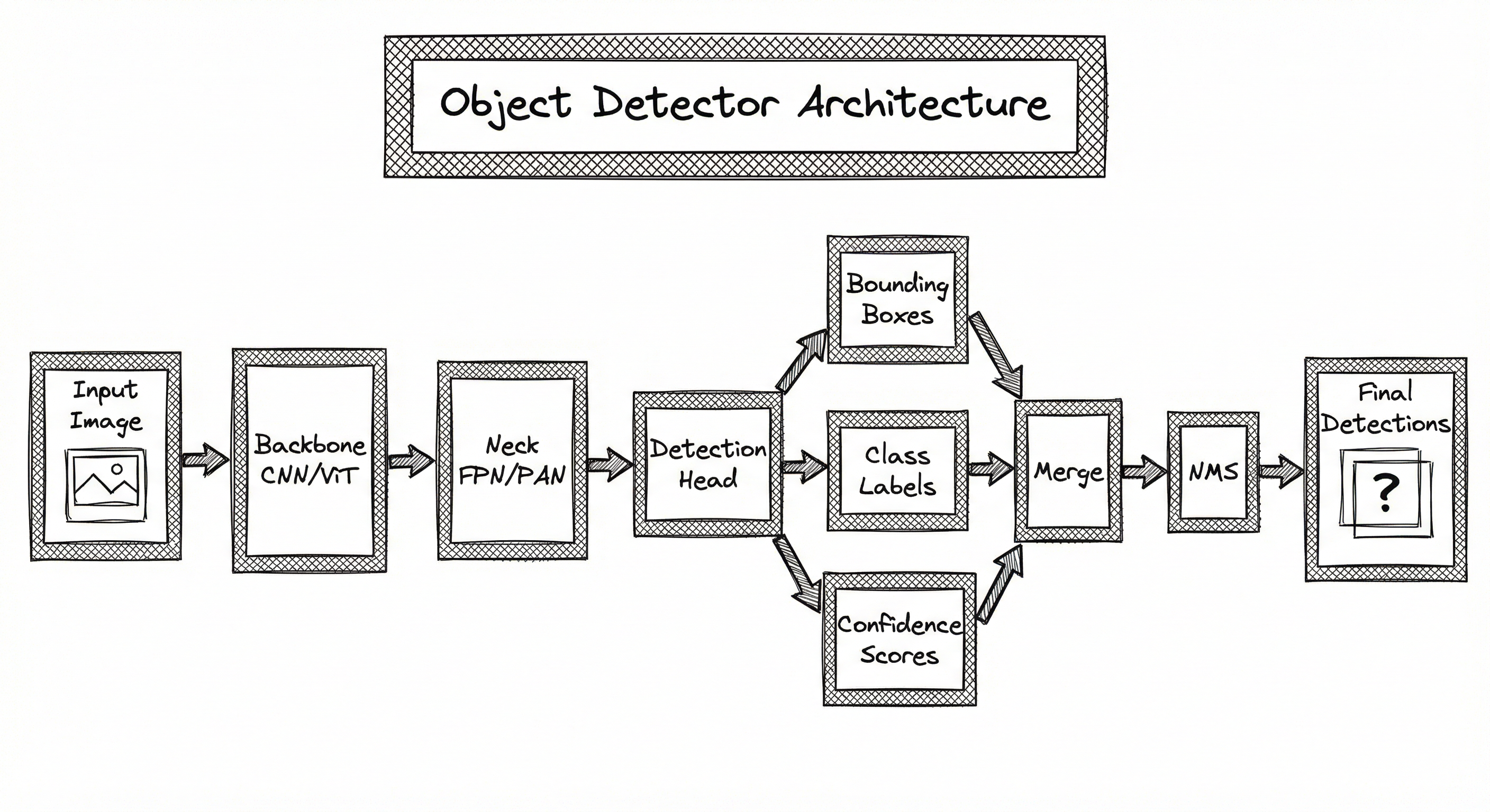
For two-stage detectors like Faster R-CNN, the head is split into a Region Proposal Network (RPN) that generates candidate boxes, followed by a per-region classifier and box regressor. For one-stage detectors like YOLO, the head directly outputs box coordinates and class probabilities at each spatial location. For DETR-style models, learned object queries attend to encoder features via cross-attention and produce detections in parallel.
Key Components
Backbone (Feature Extractor)
Extracts hierarchical feature maps from the input image at multiple resolutions. Common choices include ResNet-50/101 for two-stage detectors, CSPDarknet for YOLO variants, EfficientNet for mobile-oriented detectors, and Swin Transformer or ViT for transformer-based detectors. The backbone typically produces feature maps at strides 8, 16, and 32 relative to the input resolution.
Neck (Feature Aggregator)
Fuses multi-scale features from the backbone to create a rich, scale-invariant representation. FPN (Feature Pyramid Network) adds top-down connections for high-resolution semantics. PAN (Path Aggregation Network) adds bottom-up connections for localization precision. BiFPN (EfficientDet) adds weighted bidirectional connections. The neck is critical for detecting both large and small objects in the same image.
Detection Head
The task-specific prediction layer. In anchor-based detectors, it predicts offsets relative to predefined anchor boxes plus class probabilities. In anchor-free detectors (FCOS, CenterNet), it predicts distances from each pixel to box edges. In DETR variants, it is a transformer decoder with learned object queries that output box coordinates and class labels directly.
Region Proposal Network (RPN)
Specific to two-stage detectors like Faster R-CNN. A lightweight convolutional network that slides over the feature map and predicts objectness scores and box proposals at each location using multiple anchor sizes and aspect ratios. Outputs ~300 proposals per image, ranked by objectness score.
Post-Processing (NMS or End-to-End)
Removes duplicate detections. Traditional NMS greedily suppresses overlapping boxes based on IoU thresholds. Soft-NMS decays scores instead of hard suppression. Modern end-to-end models (DETR, YOLO26) use Hungarian matching or one-to-one label assignment during training to produce unique predictions, eliminating NMS at inference.
Label Assignment Strategy
Determines which predicted boxes are matched to ground-truth boxes during training. Anchor-based methods use IoU thresholds to assign positive/negative labels. SimOTA (used in YOLOX) dynamically assigns labels based on a cost matrix. Hungarian matching (used in DETR) finds the optimal one-to-one assignment. This component critically affects training stability and final accuracy.
Data Flow
Images and annotations (bounding boxes + labels) are loaded and augmented (mosaic, mixup, random crop, color jitter). The image passes through the backbone to produce multi-scale feature maps. The neck fuses these features. The head predicts boxes and classes. The label assignment strategy matches predictions to ground-truth. The multi-task loss (classification + localization) is computed and backpropagated.
An input image is preprocessed (resized, normalized, padded to model input size). The backbone-neck-head forward pass produces raw predictions -- typically thousands of candidate boxes. Post-processing (NMS or end-to-end filtering) removes duplicates and low-confidence predictions. The surviving detections (boxes, labels, scores) are returned.
The inference pipeline must maintain the mapping between model-space coordinates and original image coordinates. Letterbox padding, for example, shifts and scales boxes -- failing to invert this transformation is a common source of misaligned detections in production.
A directed flow diagram showing: Input Image feeds into a Backbone (CNN or Vision Transformer), which produces multi-scale feature maps. These flow into a Neck (FPN/PAN) for feature aggregation. The aggregated features enter a Detection Head that outputs three streams: Bounding Boxes, Class Labels, and Confidence Scores. These three streams converge at a Post-Processing step (NMS or End-to-End filtering), producing the Final Detections output.
How to Implement
Choosing Your Detector
The implementation landscape in 2026 offers three practical paths:
Path 1: YOLO family (Ultralytics). The most popular choice for production. YOLO26, YOLO11, and YOLOv8 offer a unified API for training, validation, export (ONNX, TensorRT, CoreML, TFLite), and deployment. If you want the fastest path from labeled data to deployed model, this is it. YOLO26-m achieves 53+ AP on COCO with NMS-free inference.
Path 2: DETR family (RT-DETR, RF-DETR). Transformer-based detectors that eliminate anchors and NMS. RF-DETR (Roboflow, 2025) achieved the first 60+ AP on COCO for a real-time model. RT-DETR (Baidu) offers excellent accuracy-speed tradeoffs. These are ideal when you need clean end-to-end pipelines and are comfortable with transformer architectures.
Path 3: Detectron2 / MMDetection (Research). Meta's Detectron2 and OpenMMLab's MMDetection provide modular frameworks for experimenting with Faster R-CNN, Cascade R-CNN, and dozens of other architectures. Best for research and benchmarking, but heavier to deploy than YOLO or RT-DETR.
For cost-sensitive deployments in India, YOLO models with TensorRT optimization on NVIDIA Jetson hardware offer the best cost-per-inference. A Jetson Orin Nano (~$249 / ~INR 21,000) can run YOLO11-s at 60+ FPS in FP16 -- sufficient for traffic monitoring, warehouse automation, or retail analytics.
Cost Note: Training a YOLO26-m model on a custom dataset of 50K images takes approximately 8-12 hours on a single NVIDIA A100 GPU. On AWS, that is about 50/month (~INR 4,200/month) total subscription cost.
from ultralytics import YOLO

# Load a pretrained YOLO26 model
model = YOLO("yolo26m.pt")

# Train on a custom dataset (COCO-format YAML)
results = model.train(
    data="custom_dataset.yaml",
    epochs=100,
    imgsz=640,
    batch=16,
    device=0,           # GPU index
    lr0=0.01,
    mosaic=1.0,
    mixup=0.15,
    close_mosaic=10,    # disable mosaic for last 10 epochs
    name="yolo26m_custom",
)

# Run inference on a single image
detections = model.predict(
    source="test_image.jpg",
    conf=0.25,          # confidence threshold
    iou=0.45,           # NMS IoU threshold (ignored if NMS-free)
    imgsz=640,
    device=0,
)

# Parse results
for det in detections:
    boxes = det.boxes.xyxy.cpu().numpy()   # (N, 4) bounding boxes
    scores = det.boxes.conf.cpu().numpy()  # (N,) confidence scores
    classes = det.boxes.cls.cpu().numpy()  # (N,) class indices
    for box, score, cls in zip(boxes, scores, classes):
        print(f"Class: {det.names[int(cls)]}, Score: {score:.2f}, Box: {box}")

# Export to TensorRT for edge deployment
model.export(format="engine", half=True, imgsz=640, device=0)
This example shows the complete workflow with Ultralytics YOLO26: loading a pretrained model, fine-tuning on custom data, running inference, and exporting to TensorRT for edge deployment. The half=True flag enables FP16 quantization, which roughly doubles throughput on NVIDIA GPUs with minimal accuracy loss (~0.2 AP). The close_mosaic parameter disables mosaic augmentation for the final training epochs, which stabilizes convergence.
import torch
import torchvision
from torchvision.models.detection import fasterrcnn_resnet50_fpn_v2, FasterRCNN_ResNet50_FPN_V2_Weights
from torchvision.models.detection.faster_rcnn import FastRCNNPredictor

# Load pretrained Faster R-CNN with ResNet-50-FPN v2 backbone
weights = FasterRCNN_ResNet50_FPN_V2_Weights.DEFAULT
model = fasterrcnn_resnet50_fpn_v2(weights=weights)

# Replace the classifier head for custom number of classes
num_classes = 5 + 1  # 5 custom classes + background
in_features = model.roi_heads.box_predictor.cls_score.in_features
model.roi_heads.box_predictor = FastRCNNPredictor(in_features, num_classes)

# Training loop (simplified)
model.train()
optimizer = torch.optim.SGD(
    model.parameters(), lr=0.005, momentum=0.9, weight_decay=0.0005
)

for epoch in range(20):
    for images, targets in train_loader:
        # targets: list of dicts with 'boxes' (FloatTensor) and 'labels' (IntTensor)
        images = [img.to("cuda") for img in images]
        targets = [{k: v.to("cuda") for k, v in t.items()} for t in targets]

        loss_dict = model(images, targets)
        total_loss = sum(loss for loss in loss_dict.values())

        optimizer.zero_grad()
        total_loss.backward()
        optimizer.step()

# Inference
model.eval()
with torch.no_grad():
    predictions = model([test_image.to("cuda")])
    # predictions[0]['boxes'], predictions[0]['labels'], predictions[0]['scores']
    for box, label, score in zip(
        predictions[0]["boxes"], predictions[0]["labels"], predictions[0]["scores"]
    ):
        if score > 0.5:
            print(f"Label: {label.item()}, Score: {score:.2f}, Box: {box.tolist()}")
This example demonstrates fine-tuning a pretrained Faster R-CNN from torchvision. Faster R-CNN remains valuable when you need high accuracy and can tolerate ~5-15 FPS inference speed -- common in offline batch processing, medical imaging, or satellite image analysis. The fasterrcnn_resnet50_fpn_v2 variant uses improved training recipes (longer training, LSJ augmentation, larger crop size) and achieves 46.7 AP on COCO, a significant jump over the original v1 weights.
from ultralytics import RTDETR

# Load a pretrained RT-DETR model
model = RTDETR("rtdetr-l.pt")

# Train on custom data
results = model.train(
    data="custom_dataset.yaml",
    epochs=80,
    imgsz=640,
    batch=8,          # transformer models need more memory per sample
    device=0,
    name="rtdetr_l_custom",
)

# Inference -- no NMS needed, end-to-end prediction
detections = model.predict(
    source="test_image.jpg",
    conf=0.5,
    imgsz=640,
)

# Evaluate on COCO-format validation set
metrics = model.val(
    data="custom_dataset.yaml",
    imgsz=640,
    batch=8,
)
print(f"[email protected]: {metrics.box.map50:.3f}")
print(f"[email protected]:0.95: {metrics.box.map:.3f}")
RT-DETR (Real-Time DEtection TRansformer) by Baidu uses a hybrid encoder combining CNN feature extraction with transformer-based attention. The key advantage is NMS-free inference: the model produces clean, deduplicated detections end-to-end. RT-DETR-L achieves 53.0 AP on COCO at 114 FPS on a T4 GPU. It is particularly strong on datasets with many overlapping objects where NMS tuning becomes painful.
import tensorrt as trt
import numpy as np
import pycuda.driver as cuda
import pycuda.autoinit

# Step 1: Export ONNX from Ultralytics (done separately)
# model.export(format="onnx", imgsz=640, half=False, simplify=True)

# Step 2: Build TensorRT engine from ONNX
def build_engine(onnx_path, engine_path, fp16=True):
    logger = trt.Logger(trt.Logger.WARNING)
    builder = trt.Builder(logger)
    network = builder.create_network(
        1 << int(trt.NetworkDefinitionCreationFlag.EXPLICIT_BATCH)
    )
    parser = trt.OnnxParser(network, logger)

    with open(onnx_path, "rb") as f:
        if not parser.parse(f.read()):
            for i in range(parser.num_errors):
                print(parser.get_error(i))
            return None

    config = builder.create_builder_config()
    config.set_memory_pool_limit(trt.MemoryPoolType.WORKSPACE, 1 << 30)  # 1 GB
    if fp16:
        config.set_flag(trt.BuilderFlag.FP16)

    engine = builder.build_serialized_network(network, config)
    with open(engine_path, "wb") as f:
        f.write(engine)
    return engine

# Step 3: Run inference with TensorRT engine
def infer(engine_path, input_data):
    logger = trt.Logger(trt.Logger.WARNING)
    with open(engine_path, "rb") as f:
        runtime = trt.Runtime(logger)
        engine = runtime.deserialize_cuda_engine(f.read())

    context = engine.create_execution_context()

    # Allocate device memory
    d_input = cuda.mem_alloc(input_data.nbytes)
    output_shape = (1, 300, 6)  # batch, max_det, (x1,y1,x2,y2,conf,cls)
    output_data = np.empty(output_shape, dtype=np.float32)
    d_output = cuda.mem_alloc(output_data.nbytes)

    cuda.memcpy_htod(d_input, input_data)
    context.execute_v2([int(d_input), int(d_output)])
    cuda.memcpy_dtoh(output_data, d_output)

    return output_data

# Usage
build_engine("yolo26m.onnx", "yolo26m_fp16.engine", fp16=True)
input_img = np.random.randn(1, 3, 640, 640).astype(np.float32)
results = infer("yolo26m_fp16.engine", input_img)
This example demonstrates the TensorRT optimization pipeline: exporting to ONNX, building a TensorRT engine with FP16 precision, and running inference. TensorRT applies layer fusion, kernel auto-tuning, and precision calibration to achieve 2-5x speedup over PyTorch inference. On an NVIDIA Jetson AGX Orin, a YOLO26-s model in FP16 can achieve 120+ FPS -- ideal for real-time edge applications like traffic monitoring or industrial inspection in India where low-cost edge devices are preferred over cloud inference.
# YOLO26 training config (YAML)
task: detect
mode: train
model: yolo26m.pt
data: custom_dataset.yaml
epochs: 100
imgsz: 640
batch: 16
device: 0
lr0: 0.01
lrf: 0.01
momentum: 0.937
weight_decay: 0.0005
warmup_epochs: 3.0
warmup_momentum: 0.8
box: 7.5
cls: 0.5
dfl: 1.5
mosaic: 1.0
mixup: 0.15
copy_paste: 0.1
close_mosaic: 10
# Augmentation
hsv_h: 0.015
hsv_s: 0.7
hsv_v: 0.4
fliplr: 0.5
translate: 0.1
scale: 0.5
# Export for edge
format: engine
half: true
int8: false
workspace: 4
Common Implementation Mistakes
- ●
Wrong input resolution: Training at 640x640 but deploying at 1280x1280 (or vice versa) without adjusting anchor sizes or retraining. The model's receptive field and feature map resolution are calibrated to the training resolution. Always match train and deploy resolutions, or use multi-scale training.
- ●
Ignoring class imbalance: COCO has 80 classes with wildly different frequencies. If your custom dataset has 95% 'car' and 5% 'motorcycle', the detector will underperform on motorcycles. Use focal loss (gamma=2.0), class-weighted sampling, or oversampling of rare classes.
- ●
NMS threshold too aggressive: Setting IoU threshold for NMS too low (e.g., 0.3) will suppress valid detections of nearby objects (e.g., people standing close together). Too high (e.g., 0.8) will produce duplicate boxes. Start with 0.45-0.65 and tune on your validation set.
- ●
Not accounting for aspect ratio in anchors: Using square anchors for detecting elongated objects (poles, trains, snakes) leads to poor localization. Either use anchor-free detectors or configure aspect ratios that match your object shape distribution.
- ●
Forgetting to invert preprocessing transforms: Letterbox padding shifts coordinates. If you do not map predicted boxes back to the original image coordinates, your detections will be offset. This is the #1 deployment bug I see in production.
- ●
Training on small images, deploying on high-res: Feeding a 4K camera stream directly to a model trained on 640x640 images wastes compute and produces poor results. Use a tiling/sliding-window approach or resize appropriately.
- ●
Ignoring small object performance: COCO AP is averaged across object sizes. If your application primarily requires small object detection (e.g., distant pedestrians, defects on PCBs), you need to specifically track AP-small and may need higher input resolution or specialized architectures like SAHI (Slicing Aided Hyper Inference).
When Should You Use This?
Use When
You need to identify and localize multiple object instances in images or video frames -- the core use case for any spatially-aware vision system
Your application requires real-time processing (30+ FPS) of camera feeds -- surveillance, robotics, autonomous driving, drone analytics
You are building an inventory management or retail analytics system that must count and track products on shelves (e.g., for a Reliance Retail or DMart deployment)
Your pipeline requires instance-level understanding as input to downstream tasks like tracking, segmentation, or action recognition
You need to detect defects, anomalies, or specific features in industrial inspection -- manufacturing QC, agricultural crop monitoring, or infrastructure inspection
You are building a visual search system where detected objects serve as query inputs (e.g., Flipkart's camera search feature)
Avoid When
You only need to know whether an object is present, not where -- use image classification instead, which is 10-50x cheaper to run
You need pixel-level boundaries, not bounding boxes -- use instance segmentation (Mask R-CNN, SAM) or semantic segmentation instead
Your objects do not have well-defined bounding boxes -- amorphous substances (smoke, fog, liquid spills) are better handled by segmentation or anomaly detection
You are working with 3D point cloud data from LiDAR -- use 3D object detectors (PointPillars, CenterPoint) rather than 2D image detectors
Your task is purely about counting identical objects in dense scenes (e.g., crowd counting) -- density estimation methods are more appropriate and efficient
You have fewer than 50-100 labeled examples per class -- consider few-shot detection methods or foundation models like Grounding DINO rather than training from scratch
Key Tradeoffs
The Speed-Accuracy Tradeoff
This is the central tension in object detection. Here is a comparison of representative models on COCO val2017:
| Model | AP@[.5:.95] | Latency (T4 GPU) | Params | Best For |
|---|---|---|---|---|
| YOLO26-n | ~38 | ~1.5ms | ~3M | Edge/mobile, real-time |
| YOLO26-m | ~53 | ~4ms | ~20M | Balanced production |
| YOLO26-l | ~55 | ~6ms | ~45M | High accuracy |
| RT-DETR-L | ~53 | ~8ms | ~32M | NMS-free, clean pipeline |
| RF-DETR-B | ~54.7 | ~5ms | ~29M | Fine-tuning champion |
| RF-DETR-2XL | ~60.6 | ~12ms | ~128M | Maximum accuracy |
| Faster R-CNN R101-FPN | ~42 | ~50ms | ~60M | Research baseline |
Input Resolution: The Hidden Multiplier
Doubling input resolution from 640 to 1280 roughly quadruples inference cost but can improve small-object AP by 5-10 points. For applications where small objects matter (distant vehicles, small defects), the resolution increase is often worth it. For applications with mostly large objects (indoor robotics), 640 is sufficient.
Anchor-Based vs. Anchor-Free
Anchor-based detectors (Faster R-CNN, YOLOv5) use predefined box templates. Anchor-free detectors (FCOS, YOLOX, YOLO26) predict directly from points. Anchor-free models are simpler to configure (no anchor hyperparameters) and often perform comparably or better. In 2026, the trend is firmly toward anchor-free.
One-Stage vs. Two-Stage
Two-stage detectors (Faster R-CNN) are more accurate on complex scenes but 5-10x slower. One-stage detectors (YOLO) are faster but historically less accurate on small or occluded objects. The gap has narrowed significantly -- YOLO26-l now exceeds Faster R-CNN's accuracy while being 10x faster.
Rule of Thumb: Start with YOLO26-m for most applications. Move to RF-DETR if you need maximum accuracy. Use Faster R-CNN only if you are doing research or need specific two-stage features (e.g., Cascade R-CNN for high-precision localization).
Alternatives & Comparisons
An image classifier assigns a single label to an entire image; an object detector localizes multiple instances with bounding boxes. If you only need presence/absence of an object (e.g., 'does this X-ray show pneumonia?'), classification is simpler, faster, and cheaper. Use detection when you need to know where and how many.
Instance segmentation (Mask R-CNN, SAM) produces pixel-level masks instead of bounding boxes. It is more precise but 2-5x more expensive. Use segmentation when you need exact object boundaries (medical imaging, autonomous driving lane markings). Use detection when bounding boxes suffice (counting, tracking, simple localization).
Face detection is a specialized form of object detection optimized for a single category. Dedicated face detectors (RetinaFace, MTCNN) incorporate facial landmark prediction and handle extreme poses, occlusion, and tiny faces better than general-purpose detectors. Use a specialized face detector when faces are your only target; use a general detector when you need faces alongside other object categories.
Image preprocessing (resizing, normalization, augmentation) is an upstream component, not an alternative. However, the choice of preprocessing directly affects detector performance. Letterbox resizing preserves aspect ratio and avoids distortion; aggressive augmentation (mosaic, mixup) can substitute for larger datasets. Always co-design preprocessing with your detector.
Pros, Cons & Tradeoffs
Advantages
Instance-level spatial understanding: Provides both classification and localization for every object in an image, enabling downstream tasks like tracking, counting, and spatial reasoning that pure classification cannot support.
Real-time capable: Modern one-stage detectors (YOLO26, RT-DETR) achieve 30-120+ FPS on consumer GPUs and edge devices, making live video processing feasible for applications like traffic monitoring in Indian smart cities.
Transfer learning efficiency: Pretrained COCO models provide strong initialization. Fine-tuning on 500-5000 domain-specific images typically yields production-quality results in hours, not weeks. This dramatically reduces data collection costs for Indian startups.
Mature ecosystem and tooling: Ultralytics, Detectron2, MMDetection, Roboflow, and CVAT provide end-to-end pipelines from annotation to deployment. You rarely need to build anything from scratch.
Multi-scale detection: FPN/PAN necks enable detecting objects across a wide range of sizes in a single forward pass -- from tiny screws in a manufacturing line to large vehicles in a parking lot.
Edge deployment maturity: TensorRT, ONNX Runtime, CoreML, and TFLite export paths are well-tested. Deploying a YOLO model to a Jetson Orin Nano (~INR 21,000 / ~$249) for production is straightforward in 2026.
Disadvantages
Bounding boxes are approximate: Rectangular boxes waste pixels on non-rectangular objects and cannot represent fine-grained boundaries. For irregular shapes (clothing items, medical lesions), segmentation is necessary.
Small object detection remains challenging: Objects smaller than 32x32 pixels on COCO are detected with ~50% lower AP than large objects. High-resolution input or tiling strategies are needed, increasing compute cost by 3-4x.
Annotation cost is high: Drawing bounding boxes is 3-5x more expensive per image than classification labels. A typical COCO-quality annotation costs INR 3-8 (~3,600-9,600).
Class imbalance sensitivity: Detectors struggle when some classes have 100x more instances than others. Focal loss helps but does not fully solve the problem. Rare classes often need targeted oversampling or synthetic data.
NMS introduces a latency floor and failure mode: Traditional NMS adds 1-5ms per image and can suppress valid detections in crowded scenes. NMS-free models solve this but are newer and less battle-tested in all deployment environments.
Domain gap is real: A model trained on COCO (mostly Western, well-lit images) may underperform on Indian street scenes with dense traffic, auto-rickshaws, and different lighting conditions. Domain-specific fine-tuning is almost always required.
Failure Modes & Debugging
Missed small objects
Cause
Input resolution too low relative to object size. At 640x640 input, objects smaller than ~16 pixels in the original image are effectively invisible to the detector because they map to sub-pixel regions on the feature maps.
Symptoms
AP-small on COCO drops below 20. Missed detections in surveillance footage for distant persons or vehicles. Users report that the system "only works when objects are close."
Mitigation
Increase input resolution to 1280 or higher. Use SAHI (Slicing Aided Hyper Inference) to tile the image and run detection on overlapping crops. Use FPN with P2-level features (stride 4) for finer resolution. Consider specialized small-object architectures.
Duplicate detections in crowded scenes
Cause
NMS threshold too permissive () or NMS failing on heavily overlapping objects of the same class (e.g., a crowd of people, stacked products on a shelf).
Symptoms
Multiple bounding boxes per object, inflated object counts. Downstream tracking algorithms receive noisy inputs and produce fragmented tracks.
Mitigation
Tune NMS threshold per-class if possible. Switch to Soft-NMS which decays scores rather than hard-suppressing. Better yet, use NMS-free models (YOLO26, DETR) that handle this end-to-end. For crowd scenarios, consider using a density estimation approach instead of detection.
Class confusion between similar categories
Cause
Insufficient visual distinction between classes in training data (e.g., 'auto-rickshaw' vs 'three-wheeler van'), or class taxonomy is too fine-grained for the model's capacity.
Symptoms
High confusion matrix values between specific class pairs. Detection scores are clustered near the decision boundary (0.4-0.6) rather than confident (>0.8).
Mitigation
Merge visually similar classes if the downstream task does not need the distinction. Add more training examples for confused classes. Use a hierarchical detection approach: detect coarse categories first, then fine-grained classification in a second stage.
False positives from background clutter
Cause
Training data does not include sufficient hard negative examples. The model has not learned what the background looks like in the deployment environment (e.g., trained on clean studio images, deployed in cluttered Indian street scenes).
Symptoms
Random background patches (textured walls, tree branches, signage) are confidently detected as objects. Precision drops while recall stays stable.
Mitigation
Collect and annotate images from the deployment environment. Use hard negative mining during training. Increase the confidence threshold at inference. Add a lightweight verification classifier after the detector.
Catastrophic performance drop on domain shift
Cause
The deployment domain differs significantly from the training domain: different camera angle, resolution, lighting, weather, or geographic context (e.g., COCO is mostly Western; Indian traffic looks very different).
Symptoms
mAP drops 15-30+ points when evaluated on deployment-domain images. The model misses common local objects (auto-rickshaws, cycle rickshaws, hand carts) not present in COCO.
Mitigation
Fine-tune on domain-specific data (even 500-1000 images help significantly). Use domain adaptation techniques (style transfer, adversarial training). For Indian deployments, consider using the Indian Driving Dataset (IDD) or annotating a custom dataset with local vehicle types.
Latency spike under load
Cause
Batch size exceeds GPU memory, triggering CPU fallback or OOM. Dynamic input shapes cause TensorRT to recompile kernels. GIL contention in Python preprocessing pipeline.
Symptoms
P99 latency jumps from 10ms to 500ms+. Inference server starts dropping frames or returning timeouts. GPU utilization oscillates between 0% and 100%.
Mitigation
Fix batch size and input resolution at export time for TensorRT. Use async preprocessing with multi-threaded data loading. Monitor GPU memory utilization and set hard limits. Use NVIDIA Triton Inference Server for production-grade request batching and scheduling.
Placement in an ML System
Where Object Detection Sits
In a perception pipeline (autonomous driving, robotics, surveillance), object detection is the first high-level inference step after raw image acquisition and preprocessing. It transforms pixel data into structured object-level information that all downstream modules consume.
For autonomous vehicles, the detector feeds into a multi-object tracker (MOT), which maintains temporal identity across frames, and a prediction module that forecasts future trajectories. The detector's recall directly determines the safety ceiling -- a missed pedestrian cannot be recovered downstream.
For retail analytics (e.g., a Reliance Retail or BigBasket deployment), the detector identifies products on shelves, feeding into a counting and planogram compliance system. Here, precision matters more -- false positives inflate inventory counts.
For visual search (e.g., Flipkart's camera search), the detector crops objects of interest from the user's photo, which are then passed to an embedding model for similarity search in a product catalog.
Key Insight: The object detector is the perceptual bottleneck of any vision pipeline. Its recall sets the ceiling for downstream task performance (you can't track what you can't detect), and its precision determines the noise floor that downstream filtering must handle.
Pipeline Stage
Inference / Perception
Upstream
- image-preprocessor
- camera-ingestion
- frame-sampler
Downstream
- object-tracker
- segmentation
- action-recognition
- scene-understanding
- face-detection
Scaling Bottlenecks
Object detection is among the most compute-intensive ML inference tasks. A single YOLO26-m inference on 640x640 input requires 50 GFLOPs. At 30 FPS across 100 camera streams, that is 150 TFLOPs/second sustained -- requiring approximately 8-10 NVIDIA T4 GPUs ($4,000/month / ~INR 3.4 lakh/month on AWS).
- Horizontal scaling: Distribute camera streams across GPU workers using a message queue (Kafka, RabbitMQ). Each worker processes a subset of streams.
- Frame skipping: Not every frame needs detection. Running at 5-10 FPS instead of 30 FPS reduces GPU cost by 3-6x. Use object tracking (DeepSORT, ByteTrack) to interpolate between detection frames.
- Model cascading: Run a tiny model (YOLO26-n) on all frames for initial screening, then a larger model (YOLO26-l) only on frames flagged as containing objects of interest.
- TensorRT + INT8 quantization: Reduces inference cost by 2-4x with 0.5-1.0 AP loss. Essential for edge deployment on Jetson devices.
For an Indian smart city deployment monitoring 500 intersections, a combination of edge inference (Jetson Orin Nano per intersection, ~INR 1.05 crore total hardware) plus cloud aggregation is typically more cost-effective than centralized cloud inference.
Production Case Studies
Tesla's official AI page describing their HydraNet architecture for vision-based object detection, which fuses 8-camera feeds through a multi-task neural network with shared backbone for detecting vehicles, pedestrians, lanes, and traffic signals.
Vision-only system deployed across Tesla fleet since 2021; Occupancy Network algorithm introduced in 2022 improved both perception accuracy and path planning for Level 2 autonomous driving (SAE).
Flipkart built a visual search and recommendation system (VisNet) that uses object detection to identify products in user-uploaded photos. The detector localizes clothing items, accessories, and furniture, then crops and embeds each detected object for similarity search against a catalog of 50M+ products. The system handles 100K+ additions/deletions per hour to the catalog, requiring continuous index updates.
Visual search powered by object detection enables Flipkart's camera search feature, allowing users to find products by photographing items in the real world. The system serves over 100 million users with sub-second response times, driving measurable increases in conversion rates for fashion and home categories.
Indian Railways is deploying AI-powered CCTV surveillance across 74,000 passenger coaches with object detection models for security monitoring. The system detects unattended baggage, suspicious activities, overcrowding, and trespassing on tracks. Detection models are optimized for Indian conditions including variable lighting, crowded platforms, and diverse clothing patterns. The deployment uses edge inference on cameras to reduce bandwidth requirements.
The system processes video feeds from thousands of cameras in real-time, flagging security events for human review. The phased rollout (completion target: 2027) represents one of the largest object detection deployments in India, covering the world's fourth-largest railway network serving 23 million passengers daily.
Waymo's perception stack combines 2D image detection with 3D LiDAR detection through sensor fusion. Their multi-frame attention network (3D-MAN) aggregates temporal context across frames for more robust 3D object detection. Waymo also pioneered large-scale auto-labeling using their offboard detection pipeline, which processes full sensor sequences offline to generate higher-quality training labels than real-time annotation.
Waymo's detection system achieves state-of-the-art 3D detection accuracy on the Waymo Open Dataset, enabling safe autonomous driving across multiple US cities. Their auto-labeling pipeline reduces per-scene annotation cost from ~0.10, a 150x reduction that makes dataset scaling feasible.
Tooling & Ecosystem
The most popular object detection framework. Provides a unified Python API and CLI for training, validation, prediction, and export across multiple YOLO versions. Supports detection, segmentation, classification, pose estimation, and OBB. Exports to ONNX, TensorRT, CoreML, TFLite, OpenVINO. AGPL-3.0 license (enterprise license available).
State-of-the-art real-time detection transformer from Roboflow. First model to exceed 60 AP on COCO in real-time. Uses neural architecture search to discover optimal accuracy-latency tradeoffs for any target dataset. Excellent for fine-tuning on custom datasets. Apache 2.0 license.
Meta's modular detection and segmentation framework. Implements Faster R-CNN, Mask R-CNN, RetinaNet, and many other architectures. Excellent for research and benchmarking but heavier to deploy than YOLO. Includes a model zoo with pretrained weights on COCO and LVIS.
Comprehensive detection toolbox with 300+ pretrained models covering all major architectures: Faster R-CNN, DETR, DINO, Co-DETR, YOLOX, and more. Modular config system makes it easy to mix and match backbones, necks, and heads. Best for systematic architecture comparison.
High-performance inference optimizer for NVIDIA GPUs. Applies layer fusion, kernel auto-tuning, FP16/INT8 quantization, and dynamic batching. Essential for production deployment on NVIDIA hardware (cloud GPUs and Jetson edge devices). Achieves 2-5x speedup over PyTorch inference.
End-to-end computer vision platform covering annotation, augmentation, training, and deployment. Provides hosted training for YOLO and RF-DETR models, auto-labeling with foundation models, and one-click deployment to edge devices. Free tier available for small projects. Popular in the Indian CV community for hackathons and prototyping.
Open-source annotation platform for bounding boxes, polygons, and keypoints. Supports collaborative annotation workflows, AI-assisted labeling, and COCO/YOLO format export. Self-hostable or available as a cloud service. Essential for building custom detection datasets.
Production inference serving platform that supports dynamic batching, model ensembling, multi-model pipelines, and GPU/CPU execution. Ideal for serving object detection models at scale with SLA guarantees. Supports TensorRT, ONNX, PyTorch, and TensorFlow backends.
Research & References
Redmon, Divvala, Girshick & Farhadi (2016)CVPR 2016
Introduced the YOLO paradigm: framing object detection as a single regression problem over a grid of cells, enabling real-time detection at 45 FPS. The foundational paper that launched the most influential family of detectors.
Ren, He, Girshick & Sun (2015)NeurIPS 2015
Introduced the Region Proposal Network (RPN) for learnable proposal generation, creating the first fully end-to-end trainable two-stage detector. Remains the conceptual foundation for understanding modern detection architectures.
Carion, Massa, Synnaeve, Usunier, Kirillov & Zagoruyko (2020)ECCV 2020
Reimagined detection as a set prediction problem using a transformer encoder-decoder with Hungarian matching. Eliminated anchors, NMS, and hand-designed components, opening a new paradigm for detection research.
Zhao, Lv, Chen, Shao, Lu, Liu, Jiang & Tang (2024)CVPR 2024
Introduced the first real-time DETR variant with a hybrid encoder architecture that achieves competitive accuracy with YOLO models while maintaining NMS-free end-to-end inference. RT-DETR-L achieves 53.0 AP at 114 FPS on T4.
Robinson, Robicheaux, Popov, Ramanan & Peri (2025)ICLR 2026
Used weight-sharing neural architecture search to discover Pareto-optimal detection transformer configurations. First real-time model to exceed 60 AP on COCO. Designed specifically for fine-tuning, achieving SOTA on custom datasets.
Lin, Dollar, Girshick, He, Hariharan & Belongie (2017)CVPR 2017
Introduced the Feature Pyramid Network (FPN) that builds a multi-scale feature representation with top-down connections. FPN is now a universal component in virtually every modern object detector.
Lin, Goyal, Girshick, He & Dollar (2017)ICCV 2017
Identified extreme foreground-background class imbalance as the cause of one-stage detectors underperforming two-stage models. Proposed focal loss to down-weight easy negatives, enabling the RetinaNet one-stage detector to match two-stage accuracy.
Tian, Shen, Chen & He (2019)ICCV 2019
Proposed an anchor-free, per-pixel detection approach where each foreground pixel directly predicts bounding box distances and a centerness score. Demonstrated that anchor-free detectors can match or exceed anchor-based performance, simplifying the detection pipeline.
Interview & Evaluation Perspective
Common Interview Questions
- ●
How would you design an object detection system for a traffic monitoring application serving 500 intersections in an Indian city?
- ●
Explain the difference between one-stage (YOLO) and two-stage (Faster R-CNN) detectors. When would you choose each?
- ●
What is the role of NMS in object detection, and how do modern architectures eliminate it?
- ●
How does DETR differ from CNN-based detectors? What are its advantages and limitations?
- ●
Walk me through how you would handle a domain shift problem -- your COCO-pretrained model performs poorly on Indian street scenes.
- ●
How do you evaluate an object detector? Explain mAP, IoU, and the difference between [email protected] and AP@[.5:.95].
- ●
How would you optimize an object detection model for edge deployment on a device with 4 TOPS of compute?
- ●
What are anchor boxes, and why are modern detectors moving away from them?
Key Points to Mention
- ●
Object detection is fundamentally a set prediction problem: variable number of outputs per image. This is what makes it architecturally more complex than classification.
- ●
The speed-accuracy tradeoff is the central design axis. Always quantify: "We need X AP at Y FPS on Z hardware." Never say "we need a fast, accurate model" without numbers.
- ●
FPN/PAN is the key architectural innovation for multi-scale detection. Understanding why multi-scale features matter (small objects need high-resolution features, large objects need large receptive fields) demonstrates deep understanding.
- ●
Focal loss solved the foreground-background imbalance problem that held back one-stage detectors. Mention the insight: easy negatives (background) dominate the loss and prevent the model from learning hard positives.
- ●
NMS elimination through one-to-one label assignment (YOLO26, DETR) simplifies deployment and removes a non-differentiable post-processing step from the pipeline. This is the industry direction in 2026.
- ●
Domain adaptation is essential for Indian deployments. COCO does not contain auto-rickshaws, cycle rickshaws, hand carts, or the traffic density typical of Indian roads. Always budget for domain-specific data collection.
- ●
TensorRT FP16/INT8 quantization is the standard optimization for NVIDIA deployment. Know the typical accuracy cost: FP16 loses ~0.2 AP, INT8 loses ~0.5-1.0 AP.
Pitfalls to Avoid
- ●
Claiming YOLO is always the best choice -- different applications have different requirements. A medical imaging system that processes 10 images/day does not need YOLO's speed.
- ●
Confusing [email protected] (PASCAL-style) with AP@[.5:.95] (COCO-style) when comparing models. A model with 75 [email protected] might only have 50 AP on COCO. Always specify the metric.
- ●
Ignoring the annotation cost of building detection datasets. Drawing bounding boxes is expensive. A senior candidate should discuss annotation strategies: semi-automated labeling, active learning, or synthetic data.
- ●
Treating NMS as a minor implementation detail. NMS is a critical design choice that affects both accuracy (crowded scenes) and latency (adds 1-5ms). Knowing when to use Soft-NMS, Weighted NMS, or NMS-free models shows depth.
- ●
Forgetting to mention data augmentation (mosaic, mixup, random crop) as a critical training component. Modern YOLO training relies heavily on augmentation -- disabling mosaic can drop AP by 2-3 points.
Senior-Level Expectation
A senior/staff-level candidate should be able to design an end-to-end detection system from data collection to production serving. This includes: (1) Data strategy -- annotation budget, active learning, domain-specific data collection for Indian conditions; (2) Model selection with quantitative justification tied to latency and accuracy requirements on target hardware; (3) Training pipeline -- augmentation strategy, learning rate schedule, distributed training for large datasets; (4) Deployment architecture -- TensorRT optimization, edge vs. cloud tradeoffs with cost analysis in INR, Triton Inference Server for batched serving, model versioning; (5) Monitoring -- mAP drift detection, latency P99 tracking, camera-specific performance analysis; (6) Failure recovery -- graceful degradation when GPU fails, fallback to lower-resolution model, alerting pipeline. The candidate should also discuss the progression from prototype (Roboflow + Google Colab) to production (distributed training on A100s + TensorRT on Jetson fleet) with realistic cost estimates.
Summary
What We Covered
Object detection is the computer vision task of identifying and localizing all instances of target object categories in an image, producing bounding boxes, class labels, and confidence scores. It is the perceptual foundation for autonomous driving, surveillance, robotics, retail analytics, and visual search systems.
The field has evolved through three paradigms: two-stage detectors (Faster R-CNN) that propose then classify regions, offering high accuracy at lower speed; one-stage detectors (YOLO family) that perform single-pass regression, offering real-time speed with competitive accuracy; and transformer-based detectors (DETR, RT-DETR, RF-DETR) that use set prediction with attention mechanisms, eliminating hand-designed components like anchors and NMS.
In 2026, the state of the art is defined by YOLO26 (NMS-free, 53+ AP, real-time) and RF-DETR (60+ AP on COCO, the first real-time model to cross this threshold). For production deployment, the Ultralytics ecosystem provides the most streamlined path from training to TensorRT-optimized edge inference. Key evaluation metrics center on mAP (COCO AP@[.5:.95]), with IoU as the geometric foundation and focal loss as the training innovation that enabled one-stage detectors to match two-stage accuracy.
For Indian deployments, the critical considerations are domain adaptation (COCO-pretrained models need fine-tuning for Indian traffic conditions, local object types, and lighting), edge deployment cost (Jetson Orin Nano at ~INR 21,000 per camera is the sweet spot), and annotation economics (budget INR 3-5 per bounding box, or use auto-labeling to reduce costs by 60-70%). The object detector is the perceptual bottleneck of any vision pipeline -- its recall sets the ceiling for all downstream tasks, making it one of the most consequential engineering decisions in an ML system.