What is the difference between Cohen's kappa and simple accuracy (raw agreement)?

**Raw agreement** (accuracy) simply counts the proportion of items on which two raters give the same label: $p_o = \text{agreements} / \text{total items}$. It does not account for the fact that some agreement happens by pure chance. **Cohen's kappa** corrects for chance agreement: $\kappa = (p_o - p_e) / (1 - p_e)$, where $p_e$ is the expected agreement if both raters labeled independently at random (preserving their individual marginal distributions). The practical difference is enormous on imbalanced data. If 90% of items belong to one class, two random raters agree about 82% of the time. Raw agreement of 85% looks decent, but kappa reveals the reality: $\kappa = (0.85 - 0.82) / (1 - 0.82) = 0.17$ -- barely above chance. Use raw agreement when class distributions are balanced (chance agreement is naturally low). Use kappa when classes are imbalanced, when comparing agreement across tasks with different label distributions, or when you need a chance-corrected quality metric for annotation pipelines.

What do different kappa values mean? How do I interpret them?

The most widely used interpretation scale is from **Landis & Koch (1977)**: | Kappa Range | Interpretation | |------------|----------------| | = 0.80 is typically required for clinical decision-making. A kappa of 0.60 might be acceptable for screening but not for definitive diagnosis. - **NLP annotation**: Kappa >= 0.60 is a common minimum for production datasets. Tasks with kappa below 0.60 typically need guideline revision. - **ML model evaluation**: Kappa > 0.40 suggests the model is doing meaningfully better than chance. Kappa > 0.70 indicates strong predictive agreement with ground truth. A negative kappa (< 0) indicates systematic disagreement -- the raters are actively contradicting each other more than random chance would predict. This usually indicates a misunderstanding of label definitions or an inverted coding scheme.

When should I use weighted kappa vs. unweighted kappa?

The choice depends entirely on whether your categories have a **natural ordering**: **Unweighted kappa**: Use for **nominal** (unordered) categories where all disagreements are equally bad. Examples: spam vs. ham vs. promotional (no natural order); cat vs. dog vs. bird; positive vs. negative vs. neutral sentiment (if you treat these as unordered). All misclassifications receive the same penalty. **Weighted kappa**: Use for **ordinal** (ordered) categories where some disagreements are worse than others. Examples: disease severity (mild/moderate/severe); star ratings (1-5); educational grades (A/B/C/D/F); Likert scales (strongly disagree to strongly agree). A 1-step disagreement (mild vs. moderate) should be penalized less than a 3-step disagreement (mild vs. critical). Within weighted kappa, you choose between: - **Linear weights**: Penalty proportional to distance. Use when all adjacent categories are equally spaced (e.g., 1-5 star ratings). - **Quadratic weights**: Penalty proportional to squared distance. Use when large disagreements are disproportionately worse (e.g., medical severity). Quadratic weighting is the default in most medical research. In scikit-learn: `cohen_kappa_score(y1, y2, weights=None)` for unweighted, `weights='linear'` for linear, `weights='quadratic'` for quadratic.

What is the kappa paradox and how should I handle it?

The **kappa paradox**, identified by Feinstein & Cicchetti (1990), occurs when raw agreement is high but kappa is low. This is not a bug in kappa -- it is a mathematically correct signal that most of the observed agreement is attributable to class prevalence rather than genuine concordance. **Why it happens**: When one class dominates (e.g., 95% negative, 5% positive), two independent raters will agree on approximately $0.95^2 + 0.05^2 = 0.9050$ of items purely by chance. If actual agreement is 0.92, kappa is only $(0.92 - 0.905) / (1 - 0.905) = 0.16$ -- slight agreement. **How to handle it**: 1. **Accept the signal**: Kappa is telling you that in a population where 95% of items are the same category, agreeing on which items are that category is not impressive. The interesting question is whether you agree on the rare 5% -- and the low kappa suggests you do not. 2. **Report positive and negative agreement separately**: $p_{pos} = 2 \cdot TP / (2 \cdot TP + FP + FN)$ measures agreement on the positive class specifically. $p_{neg} = 2 \cdot TN / (2 \cdot TN + FP + FN)$ measures agreement on the negative class. This separates the effect of prevalence. 3. **Use PABAK** (Prevalence-Adjusted Bias-Adjusted Kappa): $\text{PABAK} = 2 \cdot p_o - 1$, which removes the prevalence effect but also removes some of kappa's desirable chance correction. 4. **Consider whether the task is appropriate**: If 95% of items are trivially easy to classify and 5% require expertise, perhaps evaluate only on the challenging subset.

How does Fleiss' kappa differ from Cohen's kappa?

The key differences are: **Number of raters**: Cohen's kappa is for exactly **two** raters. Fleiss' kappa handles **any number** of raters (2 or more). **Rater assignment**: Cohen's kappa requires the **same two raters** to label all items. Fleiss' kappa allows **different raters** for different items, as long as each item receives the same number of ratings. This is critical for large annotation pipelines where annotators rotate across items. **Marginal computation**: Cohen's kappa uses each rater's individual marginal distribution to compute $p_e$. Fleiss' kappa uses the **overall proportion** of each category across all ratings. **When to use which**: - **Cohen's kappa**: Two specific raters evaluated all items (e.g., two radiologists reviewed all X-rays). Simple, well-understood, supported by sklearn. - **Fleiss' kappa**: Multiple raters, possibly rotating (e.g., each product review is labeled by 3 of 50 annotators at random). Supported by statsmodels. **Practical note**: For multi-rater scenarios, you can also compute **mean pairwise Cohen's kappa** -- average the Cohen's kappa across all rater pairs. This is simpler to compute and interpret but does not handle the rotation of raters as cleanly as Fleiss' kappa. Both approaches are commonly reported in NLP annotation studies.

How many samples do I need for a reliable kappa estimate?

The required sample size depends on the number of categories, the expected kappa, and the desired precision of the estimate. **Rules of thumb**: - **Binary classification**: At least 50 double-annotated items for a rough estimate, 200+ for a reliable estimate with narrow confidence intervals. - **K-class classification**: At least $2K^2$ items (e.g., 200 for 10 classes, 50 for 5 classes). With fewer items, rare categories may have zero observations, making kappa unreliable. - **Sim & Wright (2005)** provide formal sample size tables: to detect $\kappa = 0.60$ with 80% power against the null $\kappa = 0.40$, you need approximately 160 items for binary and 200+ for 5-category classification. **Practical guidelines for annotation pipelines**: - **Pilot study**: 50-100 double-annotated items to estimate kappa and identify problematic categories. Cheap enough to discard and redo if guidelines need revision. - **Production monitoring**: 15-20% overlap in double-annotation. For a 10,000-item dataset, that is 1,500-2,000 double-annotated items -- more than sufficient for a reliable kappa estimate. - **Rolling window**: Compute kappa on a rolling window of the last 500 double-annotated items. This provides a recent, sample-rich estimate. **Confidence interval width as a guide**: If your 95% CI spans more than 0.20 (e.g., $\kappa$ = 0.55, CI = [0.45, 0.65]), you may need more items. If it spans less than 0.10, your estimate is precise enough for most purposes.

Can I use kappa to evaluate a machine learning model, not just human annotators?

Absolutely. Cohen's kappa works for **any pair of categorical label sets** -- whether both come from human annotators, or one comes from a model and the other from ground truth. In ML evaluation, kappa measures how well the model agrees with ground truth **beyond what a random classifier would achieve given the class distribution**. **Why this is useful**: For imbalanced classification, accuracy inflates the model's apparent performance because it rewards correct predictions on the dominant class. Kappa corrects for this, just as it corrects for chance agreement between human raters. **Example**: A fraud detection model on a dataset with 1% fraud rate achieves 99.2% accuracy. Impressive? The majority-class baseline achieves 99.0%. Kappa: $(0.992 - 0.990) / (1 - 0.990) = 0.20$ -- slight agreement. The model is barely better than guessing. **Common use cases in ML**: - **Kaggle competitions**: Several Kaggle competitions (notably the Diabetic Retinopathy Detection competition) use quadratic weighted kappa as the official scoring metric because the task involves ordinal severity ratings. - **Multi-rater comparison**: Compute kappa between each model and ground truth, and between pairs of models, to understand where models agree and disagree. - **Annotation noise measurement**: Compare model predictions to each individual annotator's labels to identify which annotators' labels the model best captures. In scikit-learn, the usage is identical: `cohen_kappa_score(y_true, y_pred)` where `y_true` is ground truth and `y_pred` is the model's predictions.

What is the relationship between Cohen's kappa and Matthews Correlation Coefficient (MCC)?

Both kappa and MCC are chance-corrected metrics for classification that range from -1 to 1, with 0 indicating random performance. However, they differ in important ways: **Cohen's kappa** adjusts for chance agreement based on the raters' marginal distributions. It answers: "How much agreement is there beyond what we would expect if both raters labeled randomly with their observed base rates?" **MCC (Matthews Correlation Coefficient)** is the Pearson correlation between the actual and predicted binary labels. For a 2x2 confusion matrix: $MCC = (TP \cdot TN - FP \cdot FN) / \sqrt{(TP+FP)(TP+FN)(TN+FP)(TN+FN)}$. It answers: "How correlated are the predictions with the truth?" **Key differences**: - For **balanced data** with equal marginals, kappa and MCC are identical. - For **imbalanced data**, they can diverge because kappa uses each rater's individual marginals (which may differ), while MCC treats the confusion matrix symmetrically. - Kappa has the **maximum kappa problem**: if marginals differ, max kappa < 1.0 even with perfect agreement. MCC does not have this issue. - MCC is **symmetric** in the choice of positive/negative class. Kappa can vary depending on which class is designated positive (though this is usually irrelevant for multiclass). **When to use which**: Use kappa when the inter-rater agreement interpretation is important (annotation quality, clinical concordance). Use MCC when you want a robust single-number classifier quality metric that handles imbalance well. Both are superior to accuracy for imbalanced data.

Evaluation

Cohen's Kappa in Machine Learning

Q: When should I use weighted kappa vs. unweighted kappa?

The choice depends entirely on whether your categories have a **natural ordering**: **Unweighted kappa**: Use for **nominal** (unordered) categories where all disagreements are equally bad. Examples: spam vs. ham vs. promotional (no natural order); cat vs. dog vs. bird; positive vs. negative vs. neutral sentiment (if you treat these as unordered). All misclassifications receive the same penalty. **Weighted kappa**: Use for **ordinal** (ordered) categories where some disagreements are worse than others. Examples: disease severity (mild/moderate/severe); star ratings (1-5); educational grades (A/B/C/D/F); Likert scales (strongly disagree to strongly agree). A 1-step disagreement (mild vs. moderate) should be penalized less than a 3-step disagreement (mild vs. critical). Within weighted kappa, you choose between: - **Linear weights**: Penalty proportional to distance. Use when all adjacent categories are equally spaced (e.g., 1-5 star ratings). - **Quadratic weights**: Penalty proportional to squared distance. Use when large disagreements are disproportionately worse (e.g., medical severity). Quadratic weighting is the default in most medical research. In scikit-learn: `cohen_kappa_score(y1, y2, weights=None)` for unweighted, `weights='linear'` for linear, `weights='quadratic'` for quadratic.

Q: What is the kappa paradox and how should I handle it?

The **kappa paradox**, identified by Feinstein & Cicchetti (1990), occurs when raw agreement is high but kappa is low. This is not a bug in kappa -- it is a mathematically correct signal that most of the observed agreement is attributable to class prevalence rather than genuine concordance. **Why it happens**: When one class dominates (e.g., 95% negative, 5% positive), two independent raters will agree on approximately $0.95^2 + 0.05^2 = 0.9050$ of items purely by chance. If actual agreement is 0.92, kappa is only $(0.92 - 0.905) / (1 - 0.905) = 0.16$ -- slight agreement. **How to handle it**: 1. **Accept the signal**: Kappa is telling you that in a population where 95% of items are the same category, agreeing on which items are that category is not impressive. The interesting question is whether you agree on the rare 5% -- and the low kappa suggests you do not. 2. **Report positive and negative agreement separately**: $p_{pos} = 2 \cdot TP / (2 \cdot TP + FP + FN)$ measures agreement on the positive class specifically. $p_{neg} = 2 \cdot TN / (2 \cdot TN + FP + FN)$ measures agreement on the negative class. This separates the effect of prevalence. 3. **Use PABAK** (Prevalence-Adjusted Bias-Adjusted Kappa): $\text{PABAK} = 2 \cdot p_o - 1$, which removes the prevalence effect but also removes some of kappa's desirable chance correction. 4. **Consider whether the task is appropriate**: If 95% of items are trivially easy to classify and 5% require expertise, perhaps evaluate only on the challenging subset.

Q: How does Fleiss' kappa differ from Cohen's kappa?

The key differences are: **Number of raters**: Cohen's kappa is for exactly **two** raters. Fleiss' kappa handles **any number** of raters (2 or more). **Rater assignment**: Cohen's kappa requires the **same two raters** to label all items. Fleiss' kappa allows **different raters** for different items, as long as each item receives the same number of ratings. This is critical for large annotation pipelines where annotators rotate across items. **Marginal computation**: Cohen's kappa uses each rater's individual marginal distribution to compute $p_e$. Fleiss' kappa uses the **overall proportion** of each category across all ratings. **When to use which**: - **Cohen's kappa**: Two specific raters evaluated all items (e.g., two radiologists reviewed all X-rays). Simple, well-understood, supported by sklearn. - **Fleiss' kappa**: Multiple raters, possibly rotating (e.g., each product review is labeled by 3 of 50 annotators at random). Supported by statsmodels. **Practical note**: For multi-rater scenarios, you can also compute **mean pairwise Cohen's kappa** -- average the Cohen's kappa across all rater pairs. This is simpler to compute and interpret but does not handle the rotation of raters as cleanly as Fleiss' kappa. Both approaches are commonly reported in NLP annotation studies.

Q: How many samples do I need for a reliable kappa estimate?

The required sample size depends on the number of categories, the expected kappa, and the desired precision of the estimate. **Rules of thumb**: - **Binary classification**: At least 50 double-annotated items for a rough estimate, 200+ for a reliable estimate with narrow confidence intervals. - **K-class classification**: At least $2K^2$ items (e.g., 200 for 10 classes, 50 for 5 classes). With fewer items, rare categories may have zero observations, making kappa unreliable. - **Sim & Wright (2005)** provide formal sample size tables: to detect $\kappa = 0.60$ with 80% power against the null $\kappa = 0.40$, you need approximately 160 items for binary and 200+ for 5-category classification. **Practical guidelines for annotation pipelines**: - **Pilot study**: 50-100 double-annotated items to estimate kappa and identify problematic categories. Cheap enough to discard and redo if guidelines need revision. - **Production monitoring**: 15-20% overlap in double-annotation. For a 10,000-item dataset, that is 1,500-2,000 double-annotated items -- more than sufficient for a reliable kappa estimate. - **Rolling window**: Compute kappa on a rolling window of the last 500 double-annotated items. This provides a recent, sample-rich estimate. **Confidence interval width as a guide**: If your 95% CI spans more than 0.20 (e.g., $\kappa$ = 0.55, CI = [0.45, 0.65]), you may need more items. If it spans less than 0.10, your estimate is precise enough for most purposes.

Q: Can I use kappa to evaluate a machine learning model, not just human annotators?

Absolutely. Cohen's kappa works for **any pair of categorical label sets** -- whether both come from human annotators, or one comes from a model and the other from ground truth. In ML evaluation, kappa measures how well the model agrees with ground truth **beyond what a random classifier would achieve given the class distribution**. **Why this is useful**: For imbalanced classification, accuracy inflates the model's apparent performance because it rewards correct predictions on the dominant class. Kappa corrects for this, just as it corrects for chance agreement between human raters. **Example**: A fraud detection model on a dataset with 1% fraud rate achieves 99.2% accuracy. Impressive? The majority-class baseline achieves 99.0%. Kappa: $(0.992 - 0.990) / (1 - 0.990) = 0.20$ -- slight agreement. The model is barely better than guessing. **Common use cases in ML**: - **Kaggle competitions**: Several Kaggle competitions (notably the Diabetic Retinopathy Detection competition) use quadratic weighted kappa as the official scoring metric because the task involves ordinal severity ratings. - **Multi-rater comparison**: Compute kappa between each model and ground truth, and between pairs of models, to understand where models agree and disagree. - **Annotation noise measurement**: Compare model predictions to each individual annotator's labels to identify which annotators' labels the model best captures. In scikit-learn, the usage is identical: `cohen_kappa_score(y_true, y_pred)` where `y_true` is ground truth and `y_pred` is the model's predictions.

Q: What is the relationship between Cohen's kappa and Matthews Correlation Coefficient (MCC)?

Both kappa and MCC are chance-corrected metrics for classification that range from -1 to 1, with 0 indicating random performance. However, they differ in important ways: **Cohen's kappa** adjusts for chance agreement based on the raters' marginal distributions. It answers: "How much agreement is there beyond what we would expect if both raters labeled randomly with their observed base rates?" **MCC (Matthews Correlation Coefficient)** is the Pearson correlation between the actual and predicted binary labels. For a 2x2 confusion matrix: $MCC = (TP \cdot TN - FP \cdot FN) / \sqrt{(TP+FP)(TP+FN)(TN+FP)(TN+FN)}$. It answers: "How correlated are the predictions with the truth?" **Key differences**: - For **balanced data** with equal marginals, kappa and MCC are identical. - For **imbalanced data**, they can diverge because kappa uses each rater's individual marginals (which may differ), while MCC treats the confusion matrix symmetrically. - Kappa has the **maximum kappa problem**: if marginals differ, max kappa < 1.0 even with perfect agreement. MCC does not have this issue. - MCC is **symmetric** in the choice of positive/negative class. Kappa can vary depending on which class is designated positive (though this is usually irrelevant for multiclass). **When to use which**: Use kappa when the inter-rater agreement interpretation is important (annotation quality, clinical concordance). Use MCC when you want a robust single-number classifier quality metric that handles imbalance well. Both are superior to accuracy for imbalanced data.

Cohen's kappa ( $\kappa$ ) is the standard chance-adjusted agreement metric for classification tasks, measuring how much two raters (or a model and ground truth) agree beyond what would be expected by random chance. While accuracy answers "how often do two labelers agree?", kappa answers a far more demanding question: "how much of that agreement is genuine, after we subtract the agreement that would happen if both labelers were guessing?"

Why does this distinction matter? Consider sentiment annotation for a Flipkart product review system. If 90% of reviews are positive and two annotators each randomly label 90% as positive, they will agree 82% of the time purely by chance (0.9 x 0.9 + 0.1 x 0.1 = 0.82). Reporting 85% raw agreement sounds decent, but kappa reveals the sobering reality: $\kappa = (0.85 - 0.82) / (1 - 0.82) = 0.17$ -- barely above chance. The annotators are not really agreeing; the prevalence of the positive class is doing all the work.

This is why kappa has become the gold standard for measuring inter-annotator agreement (IAA) in NLP dataset construction, medical diagnosis inter-rater reliability, and ML model evaluation on subjective classification tasks. From Google's NLP annotation pipelines to diagnostic radiology studies at AIIMS, from Prodigy's built-in annotation metrics to scikit-learn's cohen_kappa_score, kappa is ubiquitous wherever the question is not just "do we agree?" but "do we genuinely agree?"

This guide covers the mathematical foundations of Cohen's kappa, the Landis & Koch interpretation scale, weighted kappa variants (linear and quadratic) for ordinal data, Fleiss' kappa for multiple raters, the two famous kappa paradoxes identified by Feinstein and Cicchetti, production implementation in Python, and real-world case studies from medical imaging to NLP annotation at scale.

Concept Snapshot

What It Is: A chance-adjusted agreement statistic that measures the degree to which two raters (or a classifier and ground truth) agree on categorical labels, correcting for the amount of agreement expected by random chance alone.
Category: Evaluation
Complexity: Intermediate
Inputs / Outputs: Inputs: two sets of categorical labels for the same items (from two raters, or from a model and ground truth). Outputs: a single scalar value typically between -1 and 1, where 1 = perfect agreement, 0 = agreement equal to chance, and negative values indicate agreement worse than chance.
System Placement: Sits in the evaluation stage of the ML pipeline, after predictions are generated. Particularly important in the data collection stage for measuring inter-annotator agreement (IAA) on labeled datasets, and in model evaluation for comparing model predictions against human labels on subjective tasks.
Also Known As: Kappa statistic, Kappa coefficient, Cohen's kappa coefficient, Inter-rater kappa, Agreement coefficient, Chance-corrected agreement
Typical Users: Data Scientists, ML Engineers, Annotation Team Leads, NLP Researchers, Medical Researchers, Quality Assurance Teams
Prerequisites: Confusion matrix (TP, TN, FP, FN), Binary and multiclass classification, Basic probability (marginal and joint distributions), Concept of random chance agreement
Key Terms: observed agreement (p_o)expected agreement (p_e)chance correctionLandis & Koch scaleweighted kappaFleiss' kappainter-annotator agreement (IAA)prevalence paradoxbias paradoxKrippendorff's alpha

Why This Concept Exists

The Problem: Raw Agreement Lies

In 1960, psychologist Jacob Cohen published a short but profoundly influential paper in Educational and Psychological Measurement titled "A Coefficient of Agreement for Nominal Scales." Cohen observed that researchers measuring inter-rater agreement were reporting raw percent agreement -- the fraction of items on which two raters gave the same label -- without accounting for the fact that some agreement occurs purely by chance.

The problem is analogous to accuracy on imbalanced data, but even more insidious. If two medical radiologists are asked to classify 1000 X-rays as "normal" or "abnormal," and the population prevalence of abnormality is 5%, both radiologists might independently label ~95% as normal and ~5% as abnormal. Even if they made their decisions completely independently (essentially guessing based on base rates), they would agree about 90.5% of the time: $0.95^2 + 0.05^2 = 0.9050$ . Reporting "90.5% agreement" would create the illusion of concordance where none exists.

Cohen's insight was simple but powerful: subtract the expected chance agreement from the observed agreement, then normalize by the maximum possible agreement above chance. This yields a metric where 0 means "no better than random" and 1 means "perfect agreement beyond chance."

The Evolution: From Psychology to ML

Cohen's kappa was initially adopted in psychology and medical research for measuring inter-rater reliability in diagnostic studies, behavioral coding, and clinical assessments. In 1968, Cohen extended the metric to weighted kappa to handle ordinal scales, where disagreements of different magnitudes should carry different penalties (e.g., confusing "mild" with "severe" is worse than confusing "mild" with "moderate").

In 1971, Joseph Fleiss generalized kappa to handle more than two raters in his paper "Measuring Nominal Scale Agreement Among Many Raters" published in Psychological Bulletin. Fleiss' kappa became the standard for multi-rater agreement, crucial for large-scale annotation projects where items are rated by rotating pools of annotators.

The NLP community adopted kappa in the 1990s and 2000s as corpus annotation became central to building training datasets. The landmark 2008 survey by Artstein and Poesio, "Inter-Coder Agreement for Computational Linguistics" in Computational Linguistics, systematically compared kappa, Scott's pi, and Krippendorff's alpha for annotation tasks. This paper established kappa as the default IAA metric in computational linguistics, where it remains dominant today.

The Modern Context: Annotation Quality at Scale

In the era of large language models and massive annotated datasets, kappa has taken on new urgency. Companies like Google, Meta, and OpenAI rely on human annotations for training data, evaluation benchmarks, and RLHF (Reinforcement Learning from Human Feedback). The quality of these annotations directly determines model quality, and kappa is the primary metric for measuring whether annotators are producing reliable labels.

In India, companies like Flipkart (product categorization across 40M+ products), Swiggy (restaurant cuisine classification), and Aadhaar (biometric matching quality assessment) use kappa to monitor annotation pipelines where thousands of human annotators label data at scale. A kappa score below 0.6 on an annotation task signals that the task definition is ambiguous, the annotator training is insufficient, or the task itself may be too subjective for reliable labeling -- any of which can poison downstream ML models.

Key Insight: Cohen's kappa exists because raw agreement is deceptively optimistic. In any classification task with imbalanced categories, two observers (or a model and ground truth) will agree by chance more often than you might think. Kappa strips away this inflation, revealing the genuine agreement that remains.

Core Intuition & Mental Model

The Exam Correction Analogy

Imagine you and a friend take a true/false exam where 90% of the answers are "True." If you both randomly guess "True" for every question, you will both get the same answer 82% of the time ( $0.9 \times 0.9 + 0.1 \times 0.1 = 0.82$ ). Your teacher says: "Wow, 82% agreement, you two studied together!" But you didn't -- you both exploited the same base rate.

Now suppose you actually studied and agree 91% of the time. Raw agreement says you agree 91% of the time. But Cohen's kappa says: "Hold on, 82% of that was free -- you would have gotten that just by guessing. The real question is: out of the 18% of cases where chance alone wouldn't have produced agreement, how many did you actually agree on?" The answer: $(0.91 - 0.82) / (1 - 0.82) = 0.50$ . Kappa is 0.50 -- moderate agreement at best.

This is the intuition: kappa measures how much you agree beyond what luck would give you, as a fraction of the maximum possible agreement beyond luck.

The Grading Analogy for Weighted Kappa

Now imagine grading essays on a 5-point scale (A, B, C, D, F). Two teachers grading the same essay might reasonably disagree: one gives a B, the other gives a B+. That's a small disagreement. But if one gives an A and the other gives an F, that's a massive disagreement. Standard (unweighted) kappa treats both disagreements the same -- a miss is a miss. Weighted kappa penalizes large disagreements more than small ones, which is exactly right for ordinal scales.

Linear weights penalize proportionally to distance: a 1-step disagreement (B vs. C) gets a penalty of 1, a 2-step disagreement (B vs. D) gets a penalty of 2. Quadratic weights penalize proportionally to the square of distance: a 2-step disagreement gets a penalty of 4 instead of 2, making large disagreements disproportionately costly.

Kappa as a Currency Conversion

Think of kappa as converting from a "local currency" (raw agreement, inflated by prevalence) to a "universal currency" (chance-corrected agreement, comparable across tasks). Two annotation tasks might both show 85% raw agreement, but if Task A has two equally likely categories (50:50) and Task B has one dominant category (95:5), their kappas will be very different. Task A's kappa might be 0.70 (substantial), while Task B's kappa might be 0.10 (nearly chance). Kappa normalizes away the "inflation" caused by class prevalence, making agreement scores comparable across tasks with different label distributions.

Key Insight: Raw agreement is like nominal GDP -- it looks impressive but can be inflated by factors beyond real performance. Kappa is like real GDP -- it adjusts for the "inflation" of chance agreement, revealing the genuine concordance. Always report kappa alongside raw agreement to give the full picture.

Technical Foundations

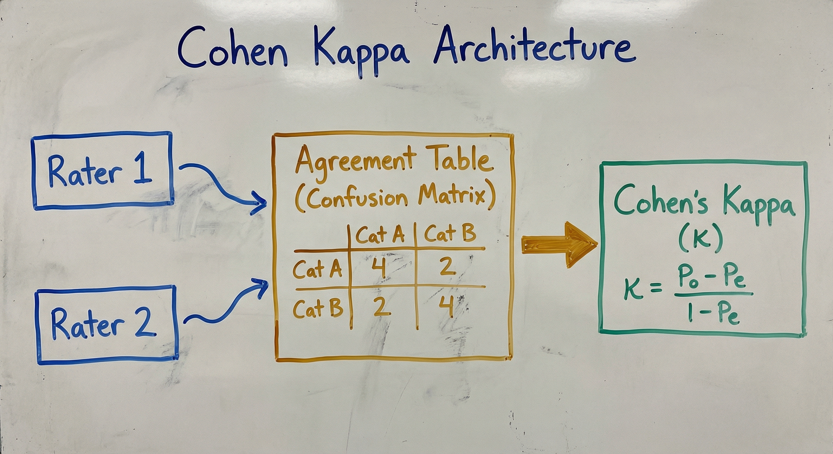
Cohen's Kappa: Binary and Multiclass

Given two raters assigning labels to $n$ items from a set of $K$ categories, let $p_o$ be the observed agreement (proportion of items on which both raters agree) and $p_e$ be the expected agreement by chance (proportion of items on which both raters would agree if they labeled independently at random, preserving their individual marginal distributions).

Cohen's kappa is defined as:

$\kappa = \frac{p_o - p_e}{1 - p_e}$

Computing $p_o$ : From the $K \times K$ agreement table (confusion matrix) where cell $n_{ij}$ is the number of items that rater 1 assigned to category $i$ and rater 2 assigned to category $j$ :

$p_o = \frac{1}{n} \sum_{k=1}^{K} n_{kk}$

This is simply the proportion of items on the main diagonal (where both raters agree).

Computing $p_e$ : Under the assumption of independence, the expected proportion of items in cell $(k, k)$ is the product of the marginal probabilities:

$p_e = \sum_{k=1}^{K} p_{k\cdot} \cdot p_{\cdot k}$

where $p_{k\cdot} = \frac{1}{n} \sum_{j=1}^{K} n_{kj}$ is the proportion of items rater 1 assigned to category $k$ , and $p_{\cdot k} = \frac{1}{n} \sum_{i=1}^{K} n_{ik}$ is the proportion of items rater 2 assigned to category $k$ .

Properties

Range: $-1 \leq \kappa \leq 1$
$\kappa = 1$ : Perfect agreement
$\kappa = 0$ : Agreement equal to chance
$\kappa < 0$ : Agreement worse than chance (systematic disagreement)
Maximum kappa can be less than 1 if the raters' marginal distributions differ, which is a known limitation

Standard Error and Confidence Intervals

The asymptotic standard error of $\kappa$ (under the null hypothesis $\kappa = 0$ ) is:

$\text{SE}_0(\kappa) = \sqrt{\frac{p_e + p_e^2 - \sum_{k=1}^{K} p_{k\cdot} \cdot p_{\cdot k} \cdot (p_{k\cdot} + p_{\cdot k})}{n \cdot (1 - p_e)^2}}$

For a 95% confidence interval: $\kappa \pm 1.96 \cdot \text{SE}(\kappa)$

Weighted Kappa for Ordinal Data

When categories are ordinal (e.g., severity ratings: mild, moderate, severe), disagreements of different magnitudes should carry different penalties. Weighted kappa generalizes kappa with a weight matrix $w_{ij}$ that assigns penalties to disagreements:

$\kappa_w = 1 - \frac{\sum_{i=1}^{K} \sum_{j=1}^{K} w_{ij} \cdot o_{ij}}{\sum_{i=1}^{K} \sum_{j=1}^{K} w_{ij} \cdot e_{ij}}$

where $o_{ij} = n_{ij} / n$ are observed proportions and $e_{ij} = p_{i\cdot} \cdot p_{\cdot j}$ are expected proportions under independence.

Linear weights (Cicchetti-Allison): Penalize proportionally to distance: $w_{ij} = \frac{|i - j|}{K - 1}$

Quadratic weights (Fleiss-Cohen): Penalize proportionally to squared distance: $w_{ij} = \frac{(i - j)^2}{(K - 1)^2}$

Linear weighted kappa is equivalent to the intraclass correlation coefficient (ICC) under certain assumptions. Quadratic weighted kappa is equivalent to the Pearson correlation coefficient between the two raters' scores under certain conditions.

Fleiss' Kappa for Multiple Raters

For $m$ raters assigning labels to $n$ items across $K$ categories, Fleiss' kappa generalizes the concept. Let $n_{ij}$ be the number of raters who assigned item $i$ to category $j$ , where $\sum_{j=1}^{K} n_{ij} = m$ for each item $i$ .

$\bar{P} = \frac{1}{n} \sum_{i=1}^{n} P_i, \quad P_i = \frac{1}{m(m-1)} \left( \sum_{j=1}^{K} n_{ij}^2 - m \right)$

$\bar{P}_e = \sum_{j=1}^{K} p_j^2, \quad p_j = \frac{1}{nm} \sum_{i=1}^{n} n_{ij}$

$\kappa_{\text{Fleiss}} = \frac{\bar{P} - \bar{P}_e}{1 - \bar{P}_e}$

Fleiss' kappa allows different raters for different items (as long as each item gets exactly $m$ ratings), making it ideal for large-scale annotation pipelines where annotators rotate across items.

Relationship to Other Metrics

Kappa is related to accuracy through the confusion matrix:

$\kappa = \frac{\text{Accuracy} - p_e}{1 - p_e}$

where accuracy is the raw observed agreement $p_o$ . When the class distribution is perfectly balanced (50:50 in binary), $p_e = 0.5$ , and kappa simplifies to $\kappa = 2 \cdot \text{Accuracy} - 1$ .

Scott's pi ( $\pi$ ) differs from Cohen's kappa in computing $p_e$ : Scott's pi uses the pooled marginal distribution (average of both raters), while Cohen's kappa uses separate marginal distributions for each rater. Scott's pi penalizes rater bias (different base rates), while Cohen's kappa does not.

Krippendorff's alpha ( $\alpha$ ) generalizes to any number of raters, handles missing data, and supports nominal, ordinal, interval, and ratio data. It is arguably the most flexible agreement coefficient but is computationally more expensive than kappa.

Internal Architecture

A Cohen's kappa computation system has four logical components: a label collector that gathers ratings from two raters (or model vs. ground truth) and ensures alignment, a contingency table builder that cross-tabulates the two sets of labels into a $K \times K$ agreement matrix, a kappa calculator that computes observed agreement ( $p_o$ ), expected agreement ( $p_e$ ), and the kappa statistic, and a result interpreter that maps the kappa value to an interpretation scale and optionally computes confidence intervals.

For large-scale annotation pipelines (as used at Flipkart, Google, and data annotation companies), the architecture extends to handle pairwise kappa computation across all annotator pairs, Fleiss' kappa for multi-rater settings, and rolling kappa monitoring to track annotation quality over time.

Cohen's Kappa in ML Systems Architecture — A vertical flow starting from 'Rater 1 Labels + Rater 2 Labels' feeding into 'Alignment & Validat...

In production annotation pipelines, the system computes kappa on a rolling basis: every 100-500 items, pairwise kappa is recomputed for active annotator pairs. If kappa drops below a threshold (typically 0.6 for classification tasks), an alert triggers retraining or task clarification.

Key Components

Label Collector & Aligner

Ingests labels from two raters (or model predictions vs. ground truth) and ensures alignment by item ID. Validates that both raters have labeled the same set of items, handles missing labels (items labeled by one rater but not the other) via exclusion or imputation, and normalizes label representations (e.g., mapping {'pos', 'positive', 'Positive'} to a canonical form). In streaming annotation pipelines, this component buffers labels until both raters have labeled each item.

Contingency Table Builder

Constructs the $K \times K$ agreement matrix where rows represent rater 1's labels and columns represent rater 2's labels. Cell $(i, j)$ contains the count of items where rater 1 assigned category $i$ and rater 2 assigned category $j$ . Computes row and column marginals for the expected agreement calculation. For weighted kappa, also constructs the weight matrix $w_{ij}$ based on the chosen weighting scheme (linear or quadratic).

Kappa Calculator

Computes the core kappa statistic from the contingency table. For unweighted kappa: sums diagonal elements for $p_o$ , computes products of marginals for $p_e$ , applies the formula $\kappa = (p_o - p_e)/(1 - p_e)$ . For weighted kappa: computes weighted observed and expected disagreement using the weight matrix. For Fleiss' kappa: handles the multi-rater generalization with item-level agreement proportions. Returns the kappa value along with $p_o$ , $p_e$ , and the contingency table for diagnostics.

Standard Error & CI Module

Computes the asymptotic standard error of kappa under the null hypothesis ( $\kappa = 0$ ) using the formula from Fleiss et al. (1969). Provides 95% confidence intervals via the normal approximation ( $\kappa \pm 1.96 \cdot SE$ ) or bootstrap resampling (more robust for small samples). Also computes the z-statistic for testing $H_0: \kappa = 0$ to determine if the observed agreement is statistically significantly different from chance.

Interpretation Engine

Maps the kappa value to a qualitative interpretation using the Landis & Koch (1977) scale: $< 0$ = Poor, $0.00-0.20$ = Slight, $0.21-0.40$ = Fair, $0.41-0.60$ = Moderate, $0.61-0.80$ = Substantial, $0.81-1.00$ = Almost Perfect. Optionally flags kappa paradoxes (high raw agreement but low kappa due to prevalence effects). Generates human-readable reports for annotation team leads and stakeholders.

Data Flow

Collection Phase: Labels from both raters are collected and aligned by item ID. The system validates that the label sets are consistent (same categories used by both raters) and handles edge cases (items labeled by only one rater, unknown category labels).

Table Construction Phase: The aligned labels are cross-tabulated into a $K \times K$ contingency table. Row and column marginals are computed. For weighted kappa, the weight matrix is constructed based on the ordinal distance between categories.

Computation Phase: The kappa calculator computes $p_o$ from the diagonal elements, $p_e$ from the marginal products, and applies the kappa formula. Standard error and confidence intervals are computed. The z-test against $\kappa = 0$ determines statistical significance.

Interpretation Phase: The kappa value is mapped to the Landis & Koch scale, compared against task-specific thresholds (e.g., $\kappa \geq 0.8$ for production annotation tasks at Flipkart), and reported alongside raw agreement, the contingency table, and per-category agreement rates. Low-kappa categories are flagged for investigation.

A vertical flow starting from 'Rater 1 Labels + Rater 2 Labels' feeding into 'Alignment & Validation', then 'K x K Contingency Table', then 'Compute Marginals' which branches to 'Observed Agreement p_o' and 'Expected Agreement p_e'. Both feed into 'Kappa = (p_o - p_e) / (1 - p_e)', which branches based on weighting type (None, Linear, Quadratic). All three paths converge to 'Interpretation & CI', which flows to 'Dashboard / Report'.

How to Implement

Implementation Approaches

Cohen's kappa computation is straightforward with scikit-learn's cohen_kappa_score, which supports unweighted, linear-weighted, and quadratic-weighted variants. For multi-rater scenarios, statsmodels provides Fleiss' kappa, and the nltk library includes agreement metrics for annotation tasks.

Option A: scikit-learn cohen_kappa_score -- the most common choice for two-rater agreement. Supports nominal (unweighted) and ordinal (linear/quadratic weighted) data. One function call, no setup required.

Option B: statsmodels cohens_kappa -- provides additional diagnostics including standard error, confidence intervals, and the z-test for $\kappa = 0$ . More verbose but more informative for research-quality reporting.

Option C: Manual implementation -- useful for understanding the math, customizing the weight matrix, or working in environments without sklearn/statsmodels. Requires only NumPy.

Option D: Fleiss' kappa via statsmodels or NLTK -- for multi-rater scenarios common in annotation pipelines where each item is labeled by 3-5 annotators.

Cost Note: Kappa computation is nearly free -- it is an $O(n)$ operation over the label pairs. The real cost is in collecting reliable labels for computing kappa. Professional annotation services in India charge approximately Rs 1-5 (INR) per label for simple classification tasks and Rs 15-50 per label for complex tasks requiring domain expertise. For a kappa study with 500 double-annotated items across 10 categories, the annotation cost is approximately Rs 1,000-25,000 (~$12-300 USD). The computation itself takes milliseconds.

Basic Cohen's Kappa with scikit-learn41 lines

from sklearn.metrics import cohen_kappa_score, confusion_matrix
import numpy as np

# Two annotators labeling 100 product reviews as positive/negative/neutral
np.random.seed(42)

# Simulate annotator labels (Flipkart review sentiment annotation)
rater_1 = np.random.choice(['positive', 'negative', 'neutral'], size=200,
                            p=[0.6, 0.25, 0.15])
rater_2 = rater_1.copy()
# Introduce ~20% disagreement
flip_indices = np.random.choice(200, size=40, replace=False)
rater_2[flip_indices] = np.random.choice(['positive', 'negative', 'neutral'],
                                          size=40, p=[0.6, 0.25, 0.15])

# Unweighted kappa (nominal categories)
kappa = cohen_kappa_score(rater_1, rater_2)
print(f"Cohen's Kappa (unweighted): {kappa:.4f}")

# Raw agreement for comparison
raw_agreement = np.mean(rater_1 == rater_2)
print(f"Raw Agreement: {raw_agreement:.4f}")

# Confusion matrix (agreement table)
labels = ['positive', 'negative', 'neutral']
cm = confusion_matrix(rater_1, rater_2, labels=labels)
print(f"\nAgreement Table (rows=rater1, cols=rater2):")
print(f"{'':>12} {'positive':>10} {'negative':>10} {'neutral':>10}")
for i, label in enumerate(labels):
    print(f"{label:>12} {cm[i, 0]:>10} {cm[i, 1]:>10} {cm[i, 2]:>10}")

# Interpretation using Landis & Koch scale
def interpret_kappa(k):
    if k < 0.00: return 'Poor (less than chance)'
    elif k < 0.20: return 'Slight'
    elif k < 0.40: return 'Fair'
    elif k < 0.60: return 'Moderate'
    elif k < 0.80: return 'Substantial'
    else: return 'Almost Perfect'

print(f"\nInterpretation: {interpret_kappa(kappa)}")

This example demonstrates the core workflow: compute kappa with cohen_kappa_score, compare it to raw agreement, inspect the confusion matrix for disagreement patterns, and interpret using the Landis & Koch scale. Notice that raw agreement is always higher than kappa would suggest -- kappa adjusts for the fact that annotators would agree on some items purely by chance given their labeling tendencies.

Weighted Kappa for Ordinal Ratings43 lines

from sklearn.metrics import cohen_kappa_score
import numpy as np

# Two radiologists rating disease severity on a 5-point ordinal scale
# 1=Normal, 2=Mild, 3=Moderate, 4=Severe, 5=Critical
np.random.seed(42)
n_cases = 300

# Simulate radiologist ratings (correlated but with noise)
true_severity = np.random.choice([1, 2, 3, 4, 5], size=n_cases,
                                  p=[0.30, 0.25, 0.20, 0.15, 0.10])
noise_1 = np.random.choice([-1, 0, 0, 0, 1], size=n_cases)
noise_2 = np.random.choice([-1, 0, 0, 0, 1], size=n_cases)
radiologist_1 = np.clip(true_severity + noise_1, 1, 5)
radiologist_2 = np.clip(true_severity + noise_2, 1, 5)

# Unweighted kappa (treats all disagreements equally)
kappa_unweighted = cohen_kappa_score(radiologist_1, radiologist_2, weights=None)
print(f"Unweighted Kappa: {kappa_unweighted:.4f}")

# Linear weighted kappa (disagreement penalty proportional to distance)
kappa_linear = cohen_kappa_score(radiologist_1, radiologist_2, weights='linear')
print(f"Linear Weighted Kappa: {kappa_linear:.4f}")

# Quadratic weighted kappa (disagreement penalty proportional to distance^2)
kappa_quadratic = cohen_kappa_score(radiologist_1, radiologist_2, weights='quadratic')
print(f"Quadratic Weighted Kappa: {kappa_quadratic:.4f}")

# Key insight: weighted > unweighted for ordinal data because
# small disagreements (e.g., Mild vs Moderate) are penalized less
# than large disagreements (e.g., Normal vs Critical)
print(f"\nDifference (quadratic - unweighted): {kappa_quadratic - kappa_unweighted:+.4f}")
print("Weighted kappa is higher because most disagreements are small (1-step)")
print("and only a few are large (2+ steps). Weighted kappa gives partial")
print("credit for near-agreements.")

# Show disagreement distribution
diffs = np.abs(radiologist_1 - radiologist_2)
print(f"\nDisagreement distribution:")
for d in range(5):
    count = np.sum(diffs == d)
    pct = count / n_cases * 100
    print(f"  {d}-step disagreement: {count:>4} ({pct:.1f}%)")

For ordinal data (disease severity, Likert scales, star ratings), weighted kappa is essential. Unweighted kappa treats a 1-step disagreement (mild vs. moderate) the same as a 4-step disagreement (normal vs. critical), which is inappropriate for ordered categories. Linear weighting penalizes proportionally to the distance between categories, while quadratic weighting penalizes proportionally to the square of the distance. In practice, quadratic weighted kappa is more commonly used in medical research, while linear weighted kappa is preferred when all adjacent categories are equally spaced.

Fleiss' Kappa for Multiple Annotators70 lines

import numpy as np
from statsmodels.stats.inter_rater import fleiss_kappa, aggregate_raters

# 5 annotators label 50 text snippets as: spam, ham, promotional
# Each item is labeled by all 5 annotators
np.random.seed(42)
n_items = 50
n_raters = 5
categories = ['spam', 'ham', 'promotional']

# Simulate annotations (mostly agree, some disagreement)
annotations = []
for i in range(n_items):
    # True category for this item
    true_cat = np.random.choice(categories, p=[0.3, 0.5, 0.2])
    # Each rater has 80% chance of choosing the true category
    item_labels = []
    for r in range(n_raters):
        if np.random.rand() < 0.80:
            item_labels.append(true_cat)
        else:
            item_labels.append(np.random.choice(categories))
    annotations.append(item_labels)

annotations = np.array(annotations)
print("Sample annotations (first 5 items):")
for i in range(5):
    print(f"  Item {i+1}: {annotations[i].tolist()}")

# Convert to category counts format required by statsmodels
# Each row: [count_cat1, count_cat2, count_cat3] for one item
category_map = {cat: idx for idx, cat in enumerate(categories)}
counts = np.zeros((n_items, len(categories)), dtype=int)
for i in range(n_items):
    for label in annotations[i]:
        counts[i, category_map[label]] += 1

print(f"\nCategory count matrix (first 5 items):")
print(f"{'':>10} {'spam':>6} {'ham':>6} {'promo':>6}")
for i in range(5):
    print(f"Item {i+1:>4}: {counts[i, 0]:>6} {counts[i, 1]:>6} {counts[i, 2]:>6}")

# Compute Fleiss' kappa
kappa_fleiss = fleiss_kappa(counts, method='fleiss')
print(f"\nFleiss' Kappa: {kappa_fleiss:.4f}")

# Interpretation
def interpret_kappa(k):
    if k < 0.00: return 'Poor'
    elif k < 0.20: return 'Slight'
    elif k < 0.40: return 'Fair'
    elif k < 0.60: return 'Moderate'
    elif k < 0.80: return 'Substantial'
    else: return 'Almost Perfect'

print(f"Interpretation: {interpret_kappa(kappa_fleiss)}")

# Pairwise Cohen's kappa for comparison
from sklearn.metrics import cohen_kappa_score

print(f"\nPairwise Cohen's Kappa (all rater pairs):")
pairwise_kappas = []
for r1 in range(n_raters):
    for r2 in range(r1 + 1, n_raters):
        k = cohen_kappa_score(annotations[:, r1], annotations[:, r2])
        pairwise_kappas.append(k)
        print(f"  Rater {r1+1} vs Rater {r2+1}: {k:.4f}")

print(f"\nMean Pairwise Cohen's Kappa: {np.mean(pairwise_kappas):.4f}")
print(f"Fleiss' Kappa:               {kappa_fleiss:.4f}")

Fleiss' kappa extends Cohen's kappa to multiple raters -- essential for production annotation pipelines where items are labeled by 3-5 annotators (e.g., at data annotation companies like iMerit, Labelbox, or in-house teams at Flipkart). The key difference: Cohen's kappa requires the same two raters for all items, while Fleiss' kappa allows different raters for different items (as long as each item gets the same number of ratings). This example also computes pairwise Cohen's kappa for comparison -- the mean pairwise kappa and Fleiss' kappa are related but not identical.

Kappa with Confidence Intervals and Hypothesis Testing84 lines

from sklearn.metrics import cohen_kappa_score
import numpy as np
from scipy import stats

def kappa_with_ci(rater_1, rater_2, weights=None, confidence=0.95, n_bootstrap=1000):
    """
    Compute Cohen's kappa with bootstrap confidence interval
    and hypothesis test for kappa = 0.
    
    Returns:
        kappa: point estimate
        ci: tuple (lower, upper) confidence interval
        p_value: p-value for test H0: kappa = 0
    """
    # Point estimate
    kappa = cohen_kappa_score(rater_1, rater_2, weights=weights)
    n = len(rater_1)
    
    # Bootstrap confidence interval
    bootstrap_kappas = []
    for _ in range(n_bootstrap):
        indices = np.random.choice(n, size=n, replace=True)
        boot_r1 = rater_1[indices]
        boot_r2 = rater_2[indices]
        try:
            boot_kappa = cohen_kappa_score(boot_r1, boot_r2, weights=weights)
            bootstrap_kappas.append(boot_kappa)
        except Exception:
            continue  # Skip degenerate bootstrap samples
    
    alpha = 1 - confidence
    ci_lower = np.percentile(bootstrap_kappas, 100 * alpha / 2)
    ci_upper = np.percentile(bootstrap_kappas, 100 * (1 - alpha / 2))
    
    # Approximate standard error from bootstrap
    se_bootstrap = np.std(bootstrap_kappas, ddof=1)
    
    # Z-test: H0: kappa = 0
    z_stat = kappa / se_bootstrap if se_bootstrap > 0 else 0
    p_value = 2 * (1 - stats.norm.cdf(abs(z_stat)))
    
    return {
        'kappa': kappa,
        'ci_lower': ci_lower,
        'ci_upper': ci_upper,
        'se': se_bootstrap,
        'z_stat': z_stat,
        'p_value': p_value,
        'n_items': n
    }

# Example: Medical diagnosis inter-rater study
np.random.seed(42)
n_patients = 150

# Two doctors classifying skin lesions
true_labels = np.random.choice(['benign', 'malignant', 'uncertain'], 
                                size=n_patients, p=[0.6, 0.25, 0.15])
doctor_1 = true_labels.copy()
doctor_2 = true_labels.copy()

# Doctor 1: 15% random disagreement
flip_1 = np.random.choice(n_patients, size=22, replace=False)
doctor_1[flip_1] = np.random.choice(['benign', 'malignant', 'uncertain'], size=22)

# Doctor 2: 12% random disagreement
flip_2 = np.random.choice(n_patients, size=18, replace=False)
doctor_2[flip_2] = np.random.choice(['benign', 'malignant', 'uncertain'], size=18)

result = kappa_with_ci(doctor_1, doctor_2, n_bootstrap=2000)

print(f"Cohen's Kappa: {result['kappa']:.4f}")
print(f"95% CI: [{result['ci_lower']:.4f}, {result['ci_upper']:.4f}]")
print(f"Standard Error: {result['se']:.4f}")
print(f"Z-statistic: {result['z_stat']:.4f}")
print(f"P-value: {result['p_value']:.6f}")
print(f"N items: {result['n_items']}")
print(f"\nConclusion: {'Significant' if result['p_value'] < 0.05 else 'Not significant'} "
      f"agreement beyond chance (p {'<' if result['p_value'] < 0.001 else '='} "
      f"{'0.001' if result['p_value'] < 0.001 else f'{result[chr(112)+chr(95)+chr(118)+chr(97)+chr(108)+chr(117)+chr(101)]:.4f}'})"
      if result['p_value'] >= 0.001 else '')
print(f"\nSignificant agreement beyond chance (p < 0.001)" 
      if result['p_value'] < 0.001 
      else f"P-value: {result['p_value']:.4f}")

In medical research and NLP annotation studies, reporting kappa without a confidence interval is incomplete. This function computes kappa with a bootstrap 95% CI and a z-test for the null hypothesis $\kappa = 0$ . A narrow CI with a significant p-value confirms genuine agreement beyond chance. A wide CI (e.g., $[0.30, 0.75]$ ) indicates you need more labeled items to pin down the true agreement level. For clinical studies published in Indian medical journals (IJMR, JAPI), reporting kappa with CI is often a requirement.

Model vs. Ground Truth Kappa for Classification Evaluation51 lines

from sklearn.metrics import cohen_kappa_score, accuracy_score, f1_score
from sklearn.metrics import classification_report
from sklearn.ensemble import RandomForestClassifier
from sklearn.datasets import make_classification
from sklearn.model_selection import train_test_split
import numpy as np

# Generate imbalanced 3-class dataset (e.g., customer support ticket routing)
X, y = make_classification(
    n_samples=2000, n_features=20, n_informative=15, n_redundant=5,
    n_classes=3, n_clusters_per_class=1,
    weights=[0.60, 0.25, 0.15],  # Imbalanced: billing 60%, tech 25%, other 15%
    random_state=42
)

class_names = ['billing', 'technical', 'other']
X_train, X_test, y_train, y_test = train_test_split(
    X, y, test_size=0.3, stratify=y, random_state=42
)

# Train model
model = RandomForestClassifier(n_estimators=100, random_state=42)
model.fit(X_train, y_train)
y_pred = model.predict(X_test)

# Compare accuracy vs. kappa
accuracy = accuracy_score(y_test, y_pred)
kappa = cohen_kappa_score(y_test, y_pred)
f1_macro = f1_score(y_test, y_pred, average='macro')

print(f"Accuracy:          {accuracy:.4f}")
print(f"Cohen's Kappa:     {kappa:.4f}")
print(f"Macro F1:          {f1_macro:.4f}")
print(f"\nAccuracy - Kappa gap: {accuracy - kappa:.4f}")
print("(Larger gap = more class imbalance inflating accuracy)")

# Full classification report
print(f"\nClassification Report:")
print(classification_report(y_test, y_pred, target_names=class_names))

# Dummy classifier baseline
from sklearn.dummy import DummyClassifier

dummy = DummyClassifier(strategy='most_frequent')
dummy.fit(X_train, y_train)
y_dummy = dummy.predict(X_test)

print(f"\nDummy Classifier (always predict majority):")
print(f"  Accuracy: {accuracy_score(y_test, y_dummy):.4f}")
print(f"  Kappa:    {cohen_kappa_score(y_test, y_dummy):.4f}")
print(f"  (Kappa correctly scores the dummy at ~0, unlike accuracy)")

Cohen's kappa is not just for inter-annotator agreement -- it works equally well for evaluating model vs. ground truth agreement on classification tasks. This is particularly valuable for imbalanced datasets where accuracy inflates. Notice how the dummy classifier achieves non-trivial accuracy (around 60% due to the dominant billing class) but kappa correctly scores it near 0, since the dummy's agreement is entirely due to chance. The gap between accuracy and kappa reveals how much of the model's apparent performance is attributable to class prevalence rather than genuine classification ability.

Configuration Example37 lines

# Annotation quality monitoring configuration (YAML)
annotation_quality:
  metrics:
    primary: cohen_kappa  # Chance-corrected agreement
    additional:
      - raw_agreement      # For reference / stakeholder reporting
      - fleiss_kappa        # When >2 annotators per item
      - krippendorff_alpha  # For tasks with missing data
  
  kappa_settings:
    weighting: null        # null for nominal, 'linear' or 'quadratic' for ordinal
    confidence_level: 0.95
    bootstrap_iterations: 1000
  
  thresholds:
    minimum_acceptable: 0.60    # Below this: task needs redesign
    target: 0.80                # Above this: production quality
    excellent: 0.90             # Above this: exceptional quality
  
  monitoring:
    compute_frequency: every_100_items  # Recompute after every 100 items
    rolling_window: 500                  # Compute over last 500 items
    alert_on_drop: true
    alert_threshold: 0.10               # Alert if kappa drops by >0.10
    compare_across_annotators: true     # Flag low-kappa annotator pairs
  
  double_annotation:
    enabled: true
    overlap_percentage: 20       # 20% of items get double-annotated
    min_overlap_items: 100       # Minimum items for reliable kappa estimate
    adjudication: expert_review  # How to resolve disagreements
  
  reporting:
    include_contingency_table: true
    include_per_category_agreement: true
    include_kappa_paradox_check: true
    interpretation_scale: landis_koch    # or 'fleiss' or 'custom'

Common Implementation Mistakes

●
Using unweighted kappa for ordinal data: When categories have a natural order (severity ratings, star reviews, Likert scales), unweighted kappa treats a 1-step disagreement (mild vs. moderate) the same as a 4-step disagreement (mild vs. critical). Always use linear or quadratic weighted kappa for ordinal data.
●
Ignoring the kappa paradox: High raw agreement with low kappa is not a bug -- it is the kappa paradox identified by Feinstein & Cicchetti (1990). When one category is highly prevalent (e.g., 95% of samples are 'negative'), raters agree by chance most of the time, and kappa correctly scores this agreement as minimal. Do not discard kappa in favor of raw agreement when this occurs.
●
Using Cohen's kappa for more than two raters: Cohen's kappa is designed for exactly two raters. For 3+ raters, use Fleiss' kappa or compute the mean pairwise Cohen's kappa. Using Cohen's kappa on aggregated multi-rater data (e.g., majority vote) loses information about inter-rater variability.
●
Not reporting confidence intervals: A kappa of 0.65 could have a 95% CI of [0.50, 0.80] or [0.62, 0.68] depending on sample size. Without CI, you cannot determine if kappa is reliably above your threshold. Always report CI, especially for sample sizes under 200.
●
Comparing kappa across tasks with different numbers of categories: Kappa is affected by the number of categories -- all else being equal, kappa tends to be lower with more categories because there are more ways to disagree. Do not directly compare kappa between a binary classification task and a 10-class classification task.
●
Confusing Cohen's kappa with Scott's pi: Both are chance-corrected agreement metrics, but they compute expected agreement differently. Cohen's kappa uses each rater's individual marginal distribution; Scott's pi uses the pooled marginal. For most ML applications, the difference is small, but be precise about which you are reporting.

When Should You Use This?

Use When

You need to measure inter-annotator agreement on a labeled dataset and want to account for the possibility that annotators agree by chance due to class prevalence
Your classification task has imbalanced categories where raw agreement (accuracy) would be inflated by the dominant class
You are comparing annotation quality across multiple tasks with different label distributions and need a metric that normalizes for base rates
Your evaluation involves subjective judgments (sentiment, severity, quality) where some baseline agreement is expected by chance and you want to measure agreement above that baseline
You need to evaluate model predictions vs. ground truth on a classification task where chance correction is important (e.g., comparing two models that both predict the majority class most of the time)
You are building an annotation quality monitoring pipeline and need a metric that is sensitive to annotator drift and degradation beyond what raw agreement captures

Avoid When

Your data has extreme class imbalance (one category >95% prevalence) -- the kappa paradox may produce counterintuitively low values despite genuinely high agreement. Consider prevalence-adjusted kappa (PABAK) or separate positive/negative agreement metrics
You have more than two raters and items are rated by different subsets -- use Fleiss' kappa (fixed number of raters per item) or Krippendorff's alpha (handles missing data and variable raters)
Your labels are continuous or interval-scaled (e.g., predicted probabilities, regression scores) -- kappa requires categorical data. Use ICC (intraclass correlation) or Bland-Altman analysis instead
You need to handle missing annotations (some items labeled by one rater but not the other) -- Cohen's kappa requires complete overlap. Use Krippendorff's alpha which handles missing data natively
Your raters have very different marginal distributions (one rater labels 80% positive, the other labels 30% positive) -- kappa may be artificially low because its maximum is constrained by marginal agreement. Investigate rater bias before interpreting kappa
You are evaluating threshold-dependent classifier performance and need a metric that varies smoothly with the decision threshold -- kappa is not designed for threshold optimization. Use ROC-AUC or PR-AUC instead

Key Tradeoffs

Kappa vs. Raw Agreement

Raw agreement (accuracy) is simple, intuitive, and always higher than kappa. It is the right metric when chance agreement is negligible (balanced classes, many categories). Kappa is the right metric when chance agreement is substantial (imbalanced classes, few categories, subjective tasks). The gap between raw agreement and kappa reveals how much of the agreement is "free" -- attributable to class prevalence rather than genuine concordance.

Scenario	Raw Agreement	Kappa	Interpretation
Balanced binary (50:50)	0.90	0.80	Genuine substantial agreement
Imbalanced binary (90:10)	0.90	0.44	Much of agreement is chance
10-class balanced	0.85	0.83	Minimal chance inflation
10-class, 1 dominant (70%)	0.85	0.78	Moderate chance inflation

Kappa vs. F1 Score

F1 score measures precision-recall balance for the positive class. Kappa measures overall chance-corrected agreement across all classes. For binary classification, F1 focuses on the positive class and ignores true negatives, while kappa considers all four quadrants of the confusion matrix. Use F1 when you care specifically about positive-class performance; use kappa when you care about overall agreement corrected for chance.

Kappa vs. Matthews Correlation Coefficient (MCC)

MCC is another chance-corrected metric that ranges from -1 to 1 and is robust to class imbalance. The key difference: MCC is symmetric in its treatment of classes (does not distinguish a "positive" class), while kappa adjusts for chance based on marginal distributions. For balanced binary data, kappa and MCC are very similar. For imbalanced data, they can diverge. MCC is preferred when you want a single quality metric for a binary classifier; kappa is preferred when the inter-rater agreement interpretation is important.

Unweighted vs. Weighted Kappa

For nominal data (categories with no natural ordering, e.g., spam/ham/promo), use unweighted kappa. For ordinal data (categories with a natural order, e.g., severity ratings, star reviews), use weighted kappa. Linear weights penalize proportionally to distance; quadratic weights penalize proportionally to squared distance. Quadratic weighted kappa is more commonly used in medical research because it gives partial credit for near-agreements.

Practical recommendation: Report kappa alongside raw agreement and the full contingency table. Use kappa for decision-making (is this annotation quality sufficient for production?), raw agreement for communication (stakeholders understand percentages), and the contingency table for diagnostics (which specific categories cause disagreement?).

Alternatives & Comparisons

Accuracy (Raw Agreement)

Accuracy measures the proportion of items where raters agree without correcting for chance. It is simpler and more intuitive but inflated by class prevalence. With 95% prevalence of one class, two random raters achieve ~90% accuracy but kappa near 0. Use accuracy for balanced data where chance correction is unnecessary; use kappa when class imbalance makes raw agreement misleading.

Confusion Matrix

The confusion matrix provides the raw cross-tabulation of labels from which kappa (and all other classification metrics) are derived. It is more informative but harder to summarize as a single number. Always inspect the confusion matrix alongside kappa to understand which specific category pairs cause disagreement. Kappa is a single-number summary of the confusion matrix that accounts for chance.

Precision, Recall, and F1 Score

F1 measures the balance between precision and recall for the positive class, ignoring true negatives. Kappa measures overall agreement corrected for chance, using all four quadrants of the confusion matrix. Use F1 when you care about positive-class performance specifically (fraud detection, disease diagnosis); use kappa when you care about overall agreement quality (annotation tasks, multi-class evaluation).

ROC-AUC

ROC-AUC is a threshold-independent metric that measures discrimination ability across all thresholds. Kappa is threshold-dependent (computed at a specific classification threshold) and measures agreement at a specific operating point. Use ROC-AUC for model comparison and threshold-independent assessment; use kappa when you need a chance-corrected agreement score at a specific threshold or for inter-rater studies.

Pros, Cons & Tradeoffs

Advantages

Chance-corrected -- unlike raw agreement, kappa adjusts for the agreement expected by random chance, making it robust to class prevalence. A kappa of 0.70 means the same thing regardless of whether the dominant class is 50% or 95% of the data
Universally understood scale -- the Landis & Koch interpretation scale (slight, fair, moderate, substantial, almost perfect) provides a standardized qualitative interpretation that is recognized across disciplines from medicine to NLP to psychology
Supports ordinal weighting -- weighted kappa (linear and quadratic) gives partial credit for near-agreements on ordinal scales, unlike accuracy which treats all disagreements equally. A 1-step disagreement on a severity scale contributes less to kappa reduction than a 4-step disagreement
Multi-rater generalization -- Fleiss' kappa extends the framework to any number of raters with rotating annotator pools, making it practical for large-scale annotation pipelines where different annotators label different items
Built into standard tooling -- sklearn.metrics.cohen_kappa_score provides one-line computation with support for unweighted, linear, and quadratic variants. Statsmodels provides Fleiss' kappa with standard errors. No custom code needed
Comparable across tasks -- because kappa normalizes for class prevalence, you can meaningfully compare agreement scores across tasks with different label distributions, unlike raw agreement which is confounded by base rates

Disadvantages

Kappa paradox -- when one class dominates (>90% prevalence), kappa can be counterintuitively low despite high raw agreement (Feinstein & Cicchetti, 1990). This is mathematically correct but practically confusing, and can lead teams to discard genuinely good agreement
Sensitive to number of categories -- kappa tends to decrease as the number of categories increases (more ways to disagree), making cross-task comparisons unfair when tasks have different numbers of labels
Maximum kappa constrained by marginals -- if two raters have different marginal distributions (e.g., one labels 70% positive, the other labels 40% positive), the maximum possible kappa is less than 1.0 even with the best possible agreement. This can penalize raters with legitimate calibration differences
Requires complete overlap -- Cohen's kappa requires both raters to label all items. Missing labels must be excluded, which can bias the estimate if missingness is non-random. Krippendorff's alpha handles missing data; kappa does not
Not threshold-independent -- for classifier evaluation, kappa is computed at a specific threshold. Changing the threshold changes kappa, confounding model quality with threshold choice. AUC-ROC is preferred for threshold-independent evaluation
Interpretation scale is somewhat arbitrary -- the Landis & Koch thresholds (0.20 for slight, 0.40 for fair, etc.) were proposed without strong statistical justification. Different disciplines use different thresholds, and what counts as 'acceptable' varies by application

Failure Modes & Debugging

Kappa Paradox: High Agreement but Low Kappa

Cause

Extreme class prevalence (one category >90% of all items) causes the expected chance agreement $p_e$ to be very high, leaving little room for kappa to exceed 0. Even if two raters agree on 92% of items, kappa may be only 0.20 because $p_e$ is already 0.90.

Symptoms

Raw agreement is high (85-95%) but kappa is low (0.10-0.30). Annotation team leads are confused because annotators appear to be doing well by percent agreement but kappa suggests poor concordance. Stakeholders lose trust in kappa as a metric.

Mitigation

Recognize the paradox: high prevalence genuinely reduces the informativeness of agreement -- most of it is free. Report both metrics: raw agreement for stakeholder communication, kappa for actual quality assessment. Use prevalence-adjusted kappa (PABAK): $(2 \cdot p_o - 1)$ adjusts for prevalence effects but loses some of kappa's chance correction. Compute positive and negative agreement separately (Cicchetti & Feinstein, 1990): $p_{pos} = 2 \cdot TP / (2 \cdot TP + FP + FN)$ and $p_{neg} = 2 \cdot TN / (2 \cdot TN + FP + FN)$ to diagnose which class drives the paradox.

Marginal Distribution Mismatch (Bias Paradox)

Cause

Two raters have different marginal distributions -- e.g., rater A labels 70% of items as positive while rater B labels only 40% as positive. This rater bias constrains the maximum possible kappa to well below 1.0, even if the raters agree on every item where they can agree.

Symptoms

Kappa is unexpectedly low despite reasonable agreement. The maximum possible kappa (given the marginals) is, say, 0.65, so a kappa of 0.55 might actually represent 85% of the achievable agreement. Without computing the maximum kappa, the result looks worse than it is.

Mitigation

Compute the maximum possible kappa given the observed marginal distributions. Report kappa as a fraction of its maximum: $\kappa / \kappa_{max}$ . Investigate rater bias: if one rater systematically labels more items as positive, they may need calibration training or the category definition may be ambiguous. Use Scott's pi instead of Cohen's kappa if you want to penalize rater bias rather than accommodate it.

Insufficient Sample Size for Reliable Kappa

Cause

Computing kappa on too few doubly-annotated items (e.g., 20-30 items) leads to wide confidence intervals and unreliable estimates. The variance of kappa increases as the number of items decreases and as the number of categories increases.

Symptoms

Kappa fluctuates dramatically between batches or time periods (0.50 in one batch, 0.80 in the next). Confidence intervals span more than 0.30 (e.g., CI = [0.35, 0.75]). Teams make contradictory decisions based on noisy kappa estimates.

Mitigation

Ensure sufficient sample size: a common rule of thumb is at least 2k^2 items per kappa estimate, where k is the number of categories (so at least 50 items for binary, 200 for a 10-class task). Report confidence intervals to quantify uncertainty. Use rolling kappa over a large window (e.g., last 500 items) rather than small batches. Sim & Wright (2005) provide sample size tables for desired kappa precision.

Misuse of Unweighted Kappa on Ordinal Data

Cause

Applying unweighted kappa to ordinal categories (e.g., disease severity: mild/moderate/severe, star ratings: 1-5) treats all disagreements equally. Confusing "mild" with "moderate" (a 1-step disagreement) is penalized the same as confusing "mild" with "severe" (a 2-step disagreement).

Symptoms

Kappa is surprisingly low even though most disagreements are small (adjacent categories). The metric does not reflect the clinical or business reality that near-agreements are more acceptable than far-agreements on ordered scales.

Mitigation

Use weighted kappa with linear or quadratic weights. Linear weights ( $w_{ij} = |i-j|/(K-1)$ ) penalize proportionally to distance. Quadratic weights ( $w_{ij} = (i-j)^2 / (K-1)^2$ ) penalize proportionally to squared distance. For medical severity scales, quadratic weighting is standard (Cohen, 1968). Always specify the weighting scheme when reporting kappa for ordinal data.

Confusing Cohen's Kappa with Fleiss' Kappa in Multi-Rater Settings

Cause

Applying Cohen's kappa to aggregated multi-rater data (e.g., computing kappa between the majority vote and each individual rater, or computing kappa on concatenated pairwise data). This violates the two-rater assumption and produces meaningless results.

Symptoms

Kappa values that do not match theoretical expectations. Inconsistencies between pairwise kappas and the reported multi-rater kappa. Disagreements appear smaller or larger than they actually are due to incorrect aggregation.

Mitigation

For multiple raters, use Fleiss' kappa (statsmodels fleiss_kappa) which correctly handles the multi-rater case. Alternatively, compute all pairwise Cohen's kappa values and report the mean pairwise kappa with standard deviation. For annotation pipelines with variable annotator assignments, use Krippendorff's alpha which handles missing data and variable numbers of raters per item.

Placement in an ML System

Where Does Kappa Sit in the Pipeline?

Cohen's kappa appears at two critical points in the ML pipeline:

1. Data Collection Stage (Inter-Annotator Agreement): Before any model is trained, kappa measures the quality of the labeled dataset. If human annotators cannot agree on labels (kappa < 0.6), the data is too noisy for reliable model training. This is the most common use of kappa in industry -- annotation teams at Flipkart, Google, and data labeling companies (iMerit, Scale AI, Labelbox) compute kappa as a standard quality metric.

The typical workflow is: define annotation guidelines -> pilot annotation (50-100 items) -> compute kappa -> revise guidelines if kappa < 0.6 -> scale annotation with 15-20% overlap -> continuous kappa monitoring.

2. Model Evaluation Stage (Model vs. Ground Truth): After model training, kappa measures how well the model agrees with ground truth, corrected for chance. This is more informative than accuracy for imbalanced classification because it reveals whether the model's correct predictions are genuine or just reflecting the base rate. A model with 95% accuracy but kappa of 0.30 on an imbalanced dataset is barely better than a majority-class predictor.

In production monitoring, kappa is tracked over time as new predictions are evaluated against delayed ground truth labels. A declining kappa signals model drift -- the model's agreement with reality is degrading, even if raw accuracy looks stable (because both the model and the baseline are tracking the same shifting class distribution).

Key Insight: Kappa is unique among evaluation metrics in being equally important at the data stage and the model stage. Poor inter-annotator kappa upstream leads to noisy labels, which leads to poor model-vs-ground-truth kappa downstream. Investing in annotation quality (higher kappa) has a direct, measurable impact on model quality.

Pipeline Stage

Evaluation / Data Quality

Upstream

confusion-matrix
train-test-split
data-annotation

Downstream

model-registry
deployment
monitoring

Scaling Bottlenecks

Where It Gets Expensive

Kappa computation itself is trivial -- O(n) time, O(K^2) space. The bottleneck is collecting double-annotated data to compute kappa on.

For offline annotation quality, the standard practice is to double-annotate 15-20% of items. For a dataset of 100,000 items at Flipkart's annotation center in Bengaluru, this means 15,000-20,000 items need two annotations. At Rs 3-5 per annotation for product categorization, the double-annotation cost is Rs 90,000-200,000 (~$1,100-2,400 USD) just for the quality measurement portion.

For production monitoring, computing kappa requires ground truth labels, which may arrive with delay (24-hour fraud confirmation at Razorpay, expert review turnaround of 1-3 days for medical imaging). This creates a monitoring lag -- kappa can only be computed on data with confirmed labels, not real-time predictions.

For large-scale multi-rater pipelines (Fleiss' kappa across 50+ annotators), computing all pairwise Cohen's kappa values grows as $O(R^2)$ where $R$ is the number of raters. With 50 raters, this is 1,225 pairwise kappa values per evaluation window. Manageable computationally, but the interpretation challenge is significant: which annotator pairs have low kappa? Is the problem with specific annotators or specific categories?

Cost-Effectiveness Tradeoff

The ROI of kappa monitoring is high: catching a drop in annotation quality early (before bad labels contaminate the training data) prevents expensive model retraining and production failures downstream. At Swiggy, a kappa monitoring system that flagged annotator drift on cuisine classification saved an estimated Rs 15-20 lakhs (~$18,000-24,000 USD) in avoided retraining costs over six months.

The pragmatic approach is tiered monitoring: compute kappa on every batch of 100 double-annotated items (fast, cheap), escalate to expert adjudication only when kappa drops below threshold (targeted, expensive). This gives continuous quality signals without requiring full double-annotation of every item.

Production Case Studies

Google (NLP Data Annotation)Technology / NLP

Google's NLP annotation pipelines (used for training models like BERT and PaLM) rely heavily on Cohen's kappa and Fleiss' kappa to measure inter-annotator agreement across tasks including sentiment analysis, named entity recognition, and toxicity classification. Each annotation task has a kappa threshold (typically 0.70+ for production datasets), and tasks below threshold undergo guideline revision and annotator retraining. The annotation team uses pairwise kappa to identify underperforming annotator pairs and category-specific kappa to identify ambiguous label definitions.

Outcome:

By enforcing kappa > 0.70 thresholds across all annotation tasks, Google's NLP team achieved 15% improvement in downstream model accuracy on tasks where annotation noise had previously been the bottleneck. The pairwise kappa monitoring system reduced annotator-related quality issues by 40%, with the biggest gains coming from identifying ambiguous category boundaries (e.g., 'sarcastic' vs. 'negative' sentiment) and revising annotation guidelines.

AIIMS / Medical Imaging ResearchHealthcare (India)

Medical imaging studies at AIIMS (All India Institute of Medical Sciences) and other Indian teaching hospitals routinely use weighted kappa to measure inter-observer agreement between radiologists on diagnostic classification tasks. A landmark study on chest X-ray classification used quadratic weighted kappa to assess agreement between two senior radiologists on a 5-point severity scale (normal, mild, moderate, severe, critical) for pulmonary disease. The study found weighted kappa of 0.78 (substantial agreement) compared to unweighted kappa of 0.62, demonstrating that most disagreements were on adjacent categories.

Outcome:

The weighted kappa analysis revealed that disagreements were concentrated at the mild-moderate boundary (41% of all disagreements), leading to revised diagnostic criteria with more specific radiographic features for each severity level. After guideline revision, weighted kappa improved from 0.78 to 0.87 (almost perfect), and the revised criteria were adopted across AIIMS diagnostic radiology departments for training junior residents.

Flipkart (Product Categorization)E-commerce (India)

Flipkart's product categorization system assigns 40M+ products to a hierarchical taxonomy of 5,000+ categories. The annotation pipeline employs 200+ annotators in Bengaluru, with 20% double-annotation for kappa monitoring. The team uses Cohen's kappa for pairwise annotator quality and Fleiss' kappa for team-level agreement. Category-specific kappa revealed that electronics subcategories (e.g., 'laptop sleeve' vs. 'laptop bag') had kappa as low as 0.45 (moderate), while clothing gender categories had kappa above 0.90 (almost perfect).

Outcome:

Kappa-driven quality improvements included: (1) splitting ambiguous categories ('laptop accessories' into 'laptop sleeve', 'laptop bag', 'laptop stand' with photo examples) which improved kappa from 0.45 to 0.78, (2) identifying and retraining 15 annotators whose pairwise kappa was consistently below 0.60, and (3) implementing automatic escalation to senior annotators when real-time kappa on a batch drops below 0.65. Overall annotation accuracy improved from 87% to 94% over six months.

Prodigy / Explosion AINLP Tooling

Prodigy, the commercial annotation tool by Explosion AI (creators of spaCy), includes built-in Cohen's kappa computation as a core feature of its annotation metrics. When multiple annotators label the same examples, Prodigy automatically computes pairwise Cohen's kappa, highlights disagreements for adjudication, and generates agreement reports. The tool recommends kappa > 0.80 for production NLP datasets and flags tasks where kappa drops below 0.60 as needing guideline revision.

Outcome:

According to Prodigy's documentation and user reports, teams using the built-in kappa monitoring reduced annotation iteration cycles by 30-40%, as they caught guideline ambiguities in pilot studies (50-100 items) rather than discovering them after annotating thousands of items. The tool's agreement report feature, showing per-category kappa alongside the full contingency table, became the standard for NLP annotation quality assurance.

Tooling & Ecosystem

scikit-learn cohen_kappa_score

PythonOpen Source

The standard Python function for computing Cohen's kappa between two sets of labels. Supports unweighted (nominal), linear weighted, and quadratic weighted kappa via the weights parameter. Accepts arrays of labels (strings or integers) and optional sample_weight. Part of sklearn.metrics. The most commonly used kappa implementation in ML.

statsmodels inter_rater (Cohen's & Fleiss' Kappa)

PythonOpen Source

Provides Cohen's kappa with standard error, confidence intervals, and z-test for $\kappa = 0$ . Also includes fleiss_kappa for multi-rater agreement and aggregate_raters for converting raw annotations to the category-count format required by Fleiss' kappa. More comprehensive than sklearn for statistical reporting.

NLTK AnnotationTask

PythonOpen Source

NLTK's agreement module provides AnnotationTask class for computing Cohen's kappa, Fleiss' kappa, Scott's pi, and Krippendorff's alpha from annotation data. Handles the standard (rater, item, label) triple format common in NLP annotation. Less efficient than sklearn for large datasets but supports more agreement coefficients natively.

Prodigy Annotation Metrics

PythonCommercial

Commercial annotation tool by Explosion AI (creators of spaCy) with built-in Cohen's kappa computation for inter-annotator agreement. Automatically computes kappa when multiple annotators label the same examples, generates agreement reports, and highlights disagreements for adjudication. Integrates directly with the annotation workflow.

irr (R Package)

ROpen Source

The standard R package for inter-rater reliability, providing kappa2() for Cohen's kappa (with weighted variants), kappam.fleiss() for Fleiss' kappa, and functions for Krippendorff's alpha, ICC, and other agreement coefficients. Widely used in medical and behavioral research. Includes standard errors and hypothesis tests.

Label Studio

PythonOpen Source

Open-source data annotation platform that supports inter-annotator agreement computation including Cohen's kappa and Krippendorff's alpha. Provides dashboards for monitoring annotation quality, annotator-level performance metrics, and agreement reports. Used by teams at Indian startups and enterprises for building labeled datasets.

Research & References

A Coefficient of Agreement for Nominal Scales

Cohen, J. (1960)Educational and Psychological Measurement, Vol. 20, No. 1, pp. 37-46

The foundational paper introducing Cohen's kappa as a chance-corrected agreement coefficient for nominal scales. Cohen argued that raw percent agreement overestimates true concordance by failing to account for chance agreement, and proposed kappa as the standard correction. This paper has over 50,000 citations and remains the definitive reference for the kappa statistic.

Weighted Kappa: Nominal Scale Agreement with Provision for Scaled Disagreement or Partial Credit

Cohen, J. (1968)Psychological Bulletin, Vol. 70, No. 4, pp. 213-220

Cohen's extension of kappa to ordinal scales using a weight matrix that assigns partial credit for near-agreements. Introduces linear and quadratic weighting schemes and shows that weighted kappa is equivalent to the intraclass correlation coefficient under certain conditions. Essential reading for medical severity rating and Likert scale applications.

Measuring Nominal Scale Agreement Among Many Raters

Fleiss, J. L. (1971)Psychological Bulletin, Vol. 76, No. 5, pp. 378-382

Generalizes Cohen's kappa from two raters to any number of raters, producing what is now known as Fleiss' kappa. The paper derives large-sample standard errors and provides a numerical example. Essential for large-scale annotation pipelines where items are labeled by rotating pools of annotators.

The Measurement of Observer Agreement for Categorical Data

Landis, J. R., & Koch, G. G. (1977)Biometrics, Vol. 33, No. 1, pp. 159-174

Introduces the widely-used interpretation scale for kappa: Poor (<0.00), Slight (0.00-0.20), Fair (0.21-0.40), Moderate (0.41-0.60), Substantial (0.61-0.80), Almost Perfect (0.81-1.00). While the thresholds are somewhat arbitrary, this scale has become the de facto standard for qualitative interpretation of kappa across all disciplines.

High Agreement but Low Kappa: I. The Problems of Two Paradoxes

Feinstein, A. R., & Cicchetti, D. V. (1990)Journal of Clinical Epidemiology, Vol. 43, No. 6, pp. 543-549

Identifies the two famous kappa paradoxes: (1) high observed agreement with low kappa due to extreme prevalence imbalance, and (2) kappa behaving differently for symmetric vs. asymmetric marginal imbalance. Proposes reporting separate positive and negative agreement alongside kappa to diagnose these paradoxes. Essential for understanding when kappa gives counterintuitive results.

Survey Article: Inter-Coder Agreement for Computational Linguistics

Artstein, R., & Poesio, M. (2008)Computational Linguistics, Vol. 34, No. 4, pp. 555-596

The definitive survey of agreement metrics for NLP corpus annotation, comparing Cohen's kappa, Scott's pi, and Krippendorff's alpha. Argues that weighted, alpha-like coefficients may be more appropriate than kappa for many annotation tasks. Covers the assumptions underlying each metric and provides practical guidance for choosing among them. Standard reference for NLP researchers.

Interview & Evaluation Perspective

Common Interview Questions

●
What is Cohen's kappa and how does it differ from simple accuracy?
●
Explain the formula for Cohen's kappa. What are p_o and p_e?
●
What is the Landis & Koch interpretation scale for kappa values?
●
When would you use weighted kappa vs. unweighted kappa?
●
What is the kappa paradox and when does it occur?
●
How does Fleiss' kappa extend Cohen's kappa to multiple raters?
●
Why is kappa important for measuring annotation quality in NLP datasets?
●
How would you compare kappa to Matthews Correlation Coefficient (MCC)?

Key Points to Mention

●
Chance correction: Kappa measures agreement beyond chance, using the formula $\kappa = (p_o - p_e)/(1 - p_e)$ . Unlike raw agreement, kappa is 0 when raters agree only as much as random chance would predict. This is critical for imbalanced datasets where chance agreement can be very high.
●
Landis & Koch scale: Know the interpretation thresholds -- slight (<0.20), fair (0.21-0.40), moderate (0.41-0.60), substantial (0.61-0.80), almost perfect (0.81-1.00). Most production annotation tasks require kappa >= 0.60 (moderate) and target >= 0.80 (substantial).
●
Weighted kappa for ordinal data: Always use weighted kappa when categories are ordered. Linear weights penalize proportionally to distance, quadratic weights penalize proportionally to squared distance. Quadratic is standard in medical research.
●
Kappa paradox: With extreme prevalence (one category >90%), kappa can be low despite high raw agreement because $p_e$ is very high. This is mathematically correct -- it means most of the agreement is attributable to the base rate, not genuine concordance.
●
Dual use: Kappa is used both at the data annotation stage (inter-annotator agreement) and the model evaluation stage (model vs. ground truth). Poor annotation kappa upstream causes poor model performance downstream.
●
Limitations: Maximum kappa is constrained by marginal distributions. Kappa is not threshold-independent. It requires complete overlap between raters (no missing data). For more flexibility, consider Krippendorff's alpha.

Pitfalls to Avoid

●
Saying kappa and accuracy are the same thing -- kappa is chance-corrected, accuracy is not. The key difference is the subtraction of expected chance agreement $p_e$
●
Not mentioning the kappa paradox when discussing limitations -- it is the most well-known issue with kappa and interviewers expect you to know about it
●
Using unweighted kappa for ordinal data without acknowledging the problem -- this conflates small and large disagreements
●
Forgetting that Cohen's kappa is for exactly two raters -- mention Fleiss' kappa for the multi-rater case
●
Treating the Landis & Koch scale as absolute truth -- it is widely used but somewhat arbitrary. Mention that acceptable kappa depends on the application context (medical diagnosis requires higher kappa than sentiment annotation)

Senior-Level Expectation

A senior candidate should demonstrate fluency with the mathematical formulation of kappa (p_o, p_e, and how p_e is computed from marginal distributions), the difference between Cohen's kappa and Scott's pi (individual vs. pooled marginals), and when to use Krippendorff's alpha instead (missing data, variable raters, interval scales). They should know the two kappa paradoxes (Feinstein & Cicchetti, 1990) and be able to explain when high agreement produces low kappa. They should have practical experience with weighted kappa for ordinal data and know the difference between linear and quadratic weighting. For annotation pipeline design, they should discuss double annotation overlap percentages (15-20% is standard), sample size requirements for reliable kappa (rule of thumb: 2k^2 items), and rolling kappa monitoring with alerting thresholds. They should understand the relationship between annotation quality (kappa) and downstream model quality, and be able to articulate how investing in higher kappa during data collection translates to better model performance and reduced retraining costs. Finally, they should know the ecosystem: sklearn cohen_kappa_score, statsmodels fleiss_kappa, and annotation tooling like Prodigy and Label Studio that provide built-in agreement metrics.

Summary

Cohen's kappa is the standard chance-adjusted agreement metric for classification, answering the question "how much do two raters agree beyond what would be expected by random chance?" Introduced by Jacob Cohen in 1960, kappa corrects the fundamental flaw of raw agreement (accuracy): on imbalanced data, two random raters will agree frequently simply because one class dominates, and raw agreement inflates this into apparent concordance. Kappa strips away this inflation with the formula $\kappa = (p_o - p_e) / (1 - p_e)$ , where $p_o$ is observed agreement and $p_e$ is expected chance agreement.

The Landis & Koch (1977) interpretation scale provides a widely-used qualitative framework: slight (<0.20), fair (0.21-0.40), moderate (0.41-0.60), substantial (0.61-0.80), and almost perfect (0.81-1.00). For ordinal data (severity ratings, star reviews), weighted kappa with linear or quadratic weights gives partial credit for near-agreements. Fleiss' kappa (1971) extends the framework to multiple raters, essential for large-scale annotation pipelines. The two kappa paradoxes identified by Feinstein & Cicchetti (1990) -- high agreement with low kappa due to extreme prevalence, and the bias paradox from marginal imbalance -- are important to recognize and handle correctly.

In ML systems, kappa serves a dual role: it measures annotation quality during dataset construction (inter-annotator agreement, typically requiring kappa >= 0.60-0.80 for production data) and model quality during evaluation (model vs. ground truth agreement, corrected for chance). Companies like Flipkart, Google, and Prodigy/Explosion AI rely on kappa monitoring to maintain annotation pipeline quality. At Indian tech companies, kappa-driven quality improvements have demonstrated measurable returns: identifying ambiguous categories, retraining underperforming annotators, and preventing noisy labels from contaminating training data.

The fundamental lesson: Raw agreement is seductive -- it is easy to compute and always looks high on imbalanced data. Cohen's kappa is the antidote: it reveals how much of that agreement is genuine and how much is attributable to class prevalence. Always report kappa alongside raw agreement for any classification task where class imbalance exists or where the question is not just "do we agree?" but "do we genuinely agree?"

Concept Snapshot

Why This Concept Exists

The Problem: Raw Agreement Lies

The Evolution: From Psychology to ML

The Modern Context: Annotation Quality at Scale

Core Intuition & Mental Model

The Exam Correction Analogy

The Grading Analogy for Weighted Kappa

Kappa as a Currency Conversion

Technical Foundations

Cohen's Kappa: Binary and Multiclass

Properties

Standard Error and Confidence Intervals

Weighted Kappa for Ordinal Data

Fleiss' Kappa for Multiple Raters

Relationship to Other Metrics

Internal Architecture

Key Components

Data Flow

How to Implement

Implementation Approaches

Common Implementation Mistakes

When Should You Use This?

Use When

Avoid When

Key Tradeoffs

Kappa vs. Raw Agreement

Kappa vs. F1 Score

Kappa vs. Matthews Correlation Coefficient (MCC)

Unweighted vs. Weighted Kappa

Alternatives & Comparisons

Pros, Cons & Tradeoffs

Advantages

Disadvantages

Failure Modes & Debugging

Kappa Paradox: High Agreement but Low Kappa

Marginal Distribution Mismatch (Bias Paradox)

Insufficient Sample Size for Reliable Kappa

Misuse of Unweighted Kappa on Ordinal Data

Confusing Cohen's Kappa with Fleiss' Kappa in Multi-Rater Settings

Placement in an ML System

Where Does Kappa Sit in the Pipeline?

Pipeline Stage

Upstream

Downstream

Scaling Bottlenecks

Production Case Studies

Tooling & Ecosystem

Research & References

Interview & Evaluation Perspective

Common Interview Questions

Key Points to Mention

Pitfalls to Avoid

Senior-Level Expectation

Summary

Related Blocks & Further Reading

Related ML Blocks

Further Reading