Novelty Score in Machine Learning
Here is a question that keeps recommendation system engineers up at night: your model has a near-perfect click-through rate -- so why are users churning?
The answer, more often than not, is boredom. Accuracy-focused recommendation systems have a fatal flaw: they converge on popular items. If everyone watches Stranger Things, the system learns to recommend Stranger Things to everyone. The model is technically "correct" -- users do click -- but the experience feels stale, predictable, and devoid of discovery. Users stop being surprised and eventually stop coming back.
Novelty Score is the metric that quantifies this problem. It measures how unfamiliar or surprising the recommended items are to the average user, using a concept borrowed directly from information theory: self-information. Items that fewer people have interacted with carry more information (are more "novel"), while popular items everyone has already seen carry less. A recommendation list full of blockbusters scores low on novelty; one that surfaces hidden gems from the long tail scores high.
Novelty sits in a family of beyond-accuracy metrics -- alongside diversity, serendipity, and coverage -- that collectively measure whether a recommendation system is doing more than just predicting clicks. From Spotify's Discover Weekly surfacing obscure artists to Flipkart promoting long-tail sellers during sale events, novelty is the metric that tells you if your system is helping users discover things they did not already know about. In this guide, we will walk through the mathematics, implementation, failure modes, and real-world applications of the novelty score, and explain exactly when (and when not) to optimize for it.
Concept Snapshot
- What It Is
- A beyond-accuracy recommendation metric that quantifies how unfamiliar or surprising recommended items are to the average user, calculated as the mean self-information (negative log-probability of item popularity) across all recommended items.
- Category
- Evaluation
- Complexity
- Intermediate
- Inputs / Outputs
- Inputs: a list of recommended items per user and a popularity distribution (interaction counts) for all items in the catalog. Outputs: a single novelty score per recommendation list, typically averaged across all users, where higher values indicate more novel (less popular) recommendations.
- System Placement
- Used during offline evaluation and A/B testing of recommendation algorithms, alongside accuracy metrics like precision, recall, and NDCG. Sits in the evaluation/monitoring layer, not the serving path.
- Also Known As
- Mean Self-Information, Expected Free Discovery, Inverse Popularity Score, Item Novelty, Surprisal Score, Recommendation Novelty
- Typical Users
- ML Engineers, Recommendation System Developers, Product Managers, Data Scientists, Content Strategy Teams
- Prerequisites
- Information theory basics (self-information, entropy), Recommendation system fundamentals, Popularity distributions and power laws, Basic probability and logarithms
- Key Terms
- self-informationinverse popularitylong-tail distributionpopularity biasmean self-informationexpected popularity complementcold-startfilter bubble
Why This Concept Exists
The Popularity Trap
Recommendation systems trained on user interaction data (clicks, purchases, ratings) inevitably suffer from popularity bias. Here is why: popular items have more interactions, which means the model has more training signal for them, which means it recommends them more confidently, which generates even more interactions. It is a self-reinforcing feedback loop.
Consider an e-commerce platform like Flipkart. During a Big Billion Days sale, 10% of products might account for 80% of all purchases. A collaborative filtering model trained on this data will learn to recommend those same popular products -- iPhones, Samsung Galaxy phones, Nike shoes -- to virtually everyone. The model achieves high accuracy (users do buy these items) but fails at discovery: a user who might have loved an artisanal leather wallet from a small seller in Jaipur will never see it.
This is not just a theoretical concern. Research consistently shows that popularity-biased systems hurt long-tail item producers (small sellers, independent artists, niche content creators) and reduce user satisfaction over time. Users who only receive popular recommendations disengage faster than those who experience discovery.
From Shannon to Recommender Systems
The mathematical foundation for novelty comes from Claude Shannon's information theory (1948). Shannon defined the self-information of an event as the negative logarithm of its probability:
The intuition is simple: a rare event carries more "information" than a common one. Hearing that it rained in Cherrapunji (very common) is not surprising -- low information. Hearing that it snowed in Chennai (extremely rare) is highly surprising -- high information.
Applied to recommendations: an item that 90% of users have already interacted with (like a top-charting Bollywood movie on JioCinema) carries very little self-information. An item that only 0.1% of users have seen (like a critically acclaimed Marathi independent film) carries a lot. The novelty metric simply averages this self-information across all recommended items.
This connection was formalized by Zhou et al. (2010) in their influential PNAS paper "Solving the Apparent Diversity-Accuracy Dilemma of Recommender Systems," where they used mean self-information as the standard novelty measure. It was further refined by Vargas and Castells (2011) at ACM RecSys, who introduced rank-awareness and relevance-weighting into the novelty framework through their Expected Popularity Complement (EPC) and Expected Free Discovery (EFD) metrics.
The Beyond-Accuracy Movement
For decades, recommendation research focused almost exclusively on accuracy: can we predict which items a user will rate highly? Metrics like RMSE, precision, recall, and NDCG dominated the landscape.
But starting around 2010, researchers began systematically studying beyond-accuracy properties: novelty, diversity, serendipity, and coverage. The landmark survey by Kaminskas and Bridge (2017) in ACM Transactions on Interactive Intelligent Systems cataloged these dimensions and showed that they independently predict user satisfaction.
The key insight: accuracy and novelty are partially orthogonal. A system can be accurate and novel -- it just requires intentional design. The challenge, as Zhou et al. demonstrated, is that naive approaches trade off accuracy for novelty. You can trivially increase novelty by recommending random obscure items, but users will hate the results. The art is boosting novelty while maintaining relevance.
Key Insight: Novelty exists because popularity bias is an inherent property of interaction-based recommendation systems. Without explicit measurement and optimization, recommender systems converge toward recommending what everyone already knows, killing discovery and eventually driving user churn.
Core Intuition & Mental Model
The Bookshop Analogy
Imagine you walk into a bookshop and ask the owner for recommendations. A popularity-focused owner says: "Everyone is reading Atomic Habits and Sapiens -- you should too." Technically accurate (these are bestsellers for a reason), but you have probably already heard of both. Zero discovery.
A novelty-focused owner says: "Have you read Piranesi by Susanna Clarke? It is a quiet, strange novel about a man living in an infinite house of statues. Not many people know about it, but readers who enjoy magical realism love it." Now that is interesting. The recommendation carries information you did not already have.
The novelty metric quantifies exactly this: how much "new information" does a recommendation carry? Recommending Sapiens (which 50% of book buyers have purchased) carries very little information -- you probably already knew about it. Recommending Piranesi (which 0.5% of buyers have purchased) carries much more -- it tells you something you did not know.
Thinking in Bits
Self-information is measured in bits (when using log base 2). An item with 50% popularity has self-information of bit. An item with 1% popularity has bits. An item with 0.01% popularity has bits.
The logarithmic scale matters. Moving from 50% popularity to 10% adds about 2.3 bits. Moving from 10% to 1% adds another 3.3 bits. Moving from 1% to 0.1% adds yet another 3.3 bits. The deeper you go into the long tail, the more information each step carries -- but the incremental gain diminishes.
This matches our intuition: the difference between "everyone knows this" and "most people know this" is small. The difference between "hardly anyone knows this" and "virtually nobody knows this" is also small. But the difference between "most people know this" and "hardly anyone knows this" is massive.
The Popularity-Novelty Seesaw
Think of novelty and popularity as sitting on opposite ends of a seesaw. Push popularity up (recommend more mainstream items) and novelty goes down. Push novelty up (recommend more obscure items) and popularity drops. The challenge for recommendation engineers is not to pick one end, but to find the balance point that maximizes long-term user satisfaction.
In practice, most real-world systems use a hybrid objective: optimize primarily for accuracy (relevance) while adding a novelty penalty or bonus term. The result is recommendations that are both relevant and surprising -- the sweet spot where users discover items they did not know they wanted.
Mental Model: Novelty measures how much your recommendation list looks like a "best-kept secrets" list versus a "top 10 most popular" list. Both have value, but systems that only produce the latter fail at the core promise of recommendation: helping users discover things they would not find on their own.
Technical Foundations
Building the Novelty Score Step by Step
Let us formalize the novelty metric from first principles, connecting each step to the intuition.
Step 1: Item Popularity
Given a catalog of items and a user-item interaction matrix, the popularity of item is defined as the fraction of users who have interacted with it:
For example, if 10,000 out of 1,000,000 users have watched a movie, . Popularity follows a power-law distribution (Zipf's law) in virtually all recommendation domains: a small number of head items have very high popularity, while a massive long tail of items has very low popularity.
Step 2: Self-Information of an Item
The self-information (or surprisal) of recommending item is:
This is directly from Shannon's information theory. Properties:
- If (everyone has seen it): novelty = 0 bits (no surprise)
- If (half the users): novelty = 1 bit
- If (1% of users): novelty 6.64 bits
- If (0.1% of users): novelty 9.97 bits
- As : novelty (infinitely surprising)
The logarithmic scaling ensures that the metric is sensitive to relative changes in popularity rather than absolute ones.
Step 3: Mean Self-Information (Basic Novelty Score)
For a recommendation list generated for user , the novelty of the list is the average self-information across all recommended items:
And the system-level novelty is the average across all users:
This is the formulation used by Zhou et al. (2010) and is the most widely cited definition of the novelty score.
Step 4: Rank-Aware Novelty (EFD)
Vargas and Castells (2011) argued that position in the recommendation list matters -- an item at position 1 has more impact than one at position 10. They introduced Expected Free Discovery (EFD), which discounts novelty by a position-dependent browsing model:
where is a discount function (e.g., , same as NDCG) and is a normalization constant.
Step 5: Relevance-Weighted Novelty
A further refinement weights novelty by relevance, so that only novel items the user actually likes contribute:
where is the binary or graded relevance of item for user . This prevents a system from gaming the novelty metric by recommending irrelevant obscure items.
Alternative Formulations
Expected Popularity Complement (EPC): Instead of log-based self-information, EPC uses as the novelty of item :
EPC is simpler and more interpretable ("what fraction of users have NOT seen this item?") but less principled than self-information because it is not rooted in information theory.
Inverse User Frequency (IUF): Analogous to IDF in text retrieval:
This is algebraically equivalent to up to a constant, so it produces the same ranking of items by novelty.
Worked Example
Suppose we have a catalog with 100,000 users and recommend 5 items to a user:
| Item | Users who interacted | ||
|---|---|---|---|
| Bollywood Blockbuster | 80,000 | 0.80 | 0.32 bits |
| Popular Thriller | 30,000 | 0.30 | 1.74 bits |
| Indie Drama | 2,000 | 0.02 | 5.64 bits |
| Regional Documentary | 500 | 0.005 | 7.64 bits |
| Obscure Short Film | 50 | 0.0005 | 10.97 bits |
For comparison, a list of 5 blockbusters (all with ) would score bits. A list of 5 extremely obscure items (all with ) would score bits. Our mixed list at 5.26 bits represents a healthy balance.
Implementation Note: The base of the logarithm (2, , 10) only changes the scale, not the relative ordering of items or lists. Base 2 is conventional in information theory (scores in bits), but any base works.
Internal Architecture
The novelty score is a metric, not a deployable service, but there is a clear computational architecture for how it integrates into a recommendation evaluation pipeline. The key data dependency is the popularity distribution, which must be computed from the training set (not the test set) to avoid information leakage.
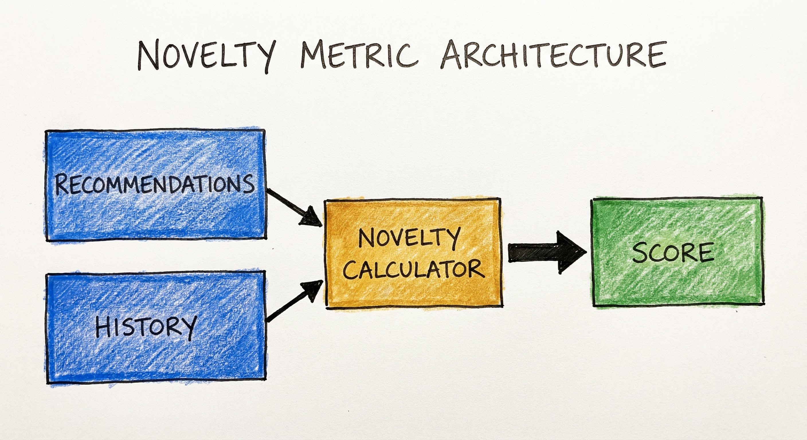
The architecture has two parallel paths: one computing the popularity distribution from historical data, and one generating recommendation lists from the model. These converge at the novelty calculator, which applies the self-information formula to produce per-user and aggregate scores.
Key Components
Popularity Calculator
Computes the popularity distribution for every item in the catalog by counting the number of distinct users who interacted with each item, divided by the total number of users. Uses training set interactions only to avoid leakage. Must handle time-windowed popularity (e.g., last 30 days) for domains where popularity shifts rapidly.
Recommendation Model
Any recommendation algorithm (collaborative filtering, content-based, hybrid, neural) that produces a ranked list of top-K items for each user. The novelty metric is model-agnostic -- it evaluates the output, not the internals.
Novelty Calculator
Takes each user's recommended list and the global popularity distribution, computes for each recommended item, and averages across the list. Optionally applies rank discounting (EFD) or relevance weighting. Handles edge cases like unseen items (no interactions) and items with zero popularity.
Aggregation Layer
Averages per-user novelty scores across the entire user population to produce the system-level novelty score. May also compute novelty segmented by user cohort (new users vs. power users), item category, or time period.
Evaluation Dashboard
Displays novelty alongside accuracy metrics (precision, NDCG), other beyond-accuracy metrics (diversity, coverage, serendipity), and business metrics (CTR, conversion, retention). Enables comparison across model variants in A/B tests.
Data Flow
The data flow for novelty computation follows these steps:
Offline preparation (run once per training cycle):
- Load user-item interaction matrix from the training set
- For each item , count distinct users who interacted:
- Compute popularity:
- Precompute self-information:
- Store as a lookup table: item_id -> self_information
Per-model evaluation:
- For each user , generate top-K recommendation list
- For each item , look up
- Compute list novelty:
- Average across users:
Online evaluation (A/B testing):
- Log which items are shown and which are interacted with
- Periodically recompute popularity from recent interactions
- Compute novelty for each treatment group
- Compare novelty alongside engagement metrics to assess trade-offs
A directed flow showing two input sources: 'Item Catalog' and 'Interaction Logs' feeding into a 'Popularity Calculator' that produces 'Popularity Distribution'. In parallel, a 'Recommendation Model' produces 'Recommended Lists'. Both outputs feed into a 'Novelty Calculator', which produces 'Per-User Novelty' scores, aggregated into a 'Mean Novelty Score' displayed on an 'Evaluation Dashboard' that informs 'A/B Test Decisions'.
How to Implement
Three Approaches to Computing Novelty
The novelty score is straightforward to implement because it requires only two inputs: recommendation lists and item popularity counts. Unlike metrics that need ground-truth relevance labels (NDCG, MAP), novelty is computed entirely from interaction data you already have.
Option A: From scratch in NumPy -- simplest approach, full control, works for any recommendation framework. Takes about 20 lines of code. Ideal for custom pipelines.
Option B: Use RecBole -- the most comprehensive recommendation evaluation library, supports novelty (mean self-information) out of the box alongside 30+ other metrics. Best for academic research and benchmarking.
Option C: Use Cornac or recmetrics -- lightweight alternatives when you do not need the full RecBole ecosystem. Cornac is better for multimodal recommenders; recmetrics is the smallest library.
For production systems at Indian tech companies, Option A is most common because it integrates directly into existing evaluation pipelines (Spark, Airflow, internal frameworks) without adding a heavy dependency.
Cost Note: Computing novelty is essentially free -- it is basic arithmetic over precomputed popularity values. The computational cost is dominated by generating the recommendations themselves (model inference), not evaluating them. For 1 million users with top-10 lists, novelty computation takes under 1 second on a single CPU core. Storage for the popularity lookup table is negligible (one float per item -- for a catalog of 10 million items, that is about 40 MB).
import numpy as np
from collections import Counter

def compute_item_popularity(interactions, n_users):
    """Compute popularity p(i) for each item.

    Args:
        interactions: list of (user_id, item_id) tuples
        n_users: total number of users in the system

    Returns:
        dict mapping item_id -> popularity p(i)
    """
    item_user_counts = Counter()
    seen_pairs = set()
    for user_id, item_id in interactions:
        if (user_id, item_id) not in seen_pairs:
            item_user_counts[item_id] += 1
            seen_pairs.add((user_id, item_id))

    return {item_id: count / n_users
            for item_id, count in item_user_counts.items()}

def novelty_score(recommendations, popularity, log_base=2):
    """Compute mean self-information novelty score.

    Args:
        recommendations: dict mapping user_id -> list of recommended item_ids
        popularity: dict mapping item_id -> p(i) (fraction of users)
        log_base: base of logarithm (2 for bits, e for nats)

    Returns:
        float: system-level novelty score (mean self-information)
    """
    user_novelties = []

    for user_id, rec_list in recommendations.items():
        item_novelties = []
        for item_id in rec_list:
            p_i = popularity.get(item_id, 1e-10)  # small epsilon for unseen items
            self_info = -np.log(p_i) / np.log(log_base)
            item_novelties.append(self_info)

        if item_novelties:
            user_novelties.append(np.mean(item_novelties))

    return np.mean(user_novelties) if user_novelties else 0.0

# Example usage
interactions = [
    ('u1', 'item_a'), ('u1', 'item_b'), ('u1', 'item_c'),
    ('u2', 'item_a'), ('u2', 'item_d'),
    ('u3', 'item_a'), ('u3', 'item_b'), ('u3', 'item_e'),
    ('u4', 'item_a'), ('u4', 'item_c'),
    ('u5', 'item_a'),
]
n_users = 5

popularity = compute_item_popularity(interactions, n_users)
print("Item popularity:")
for item, p in sorted(popularity.items()):
    print(f"  {item}: p={p:.2f}, novelty={-np.log2(p):.2f} bits")

# item_a: p=1.00 -> 0.00 bits (everyone has seen it)
# item_b: p=0.40 -> 1.32 bits
# item_c: p=0.40 -> 1.32 bits
# item_d: p=0.20 -> 2.32 bits
# item_e: p=0.20 -> 2.32 bits

recommendations = {
    'u1': ['item_d', 'item_e'],          # novel items
    'u2': ['item_b', 'item_c', 'item_e'],# mix
    'u3': ['item_a', 'item_d'],          # popular + novel
}

score = novelty_score(recommendations, popularity)
print(f"\nSystem novelty: {score:.2f} bits")
# System novelty: 1.65 bits
This implementation follows the standard mean self-information formula from Zhou et al. (2010). We first compute the popularity distribution from training interactions (counting distinct user-item pairs to avoid duplicate inflation), then compute the average negative log-probability across each user's recommendation list. The 1e-10 epsilon handles cold-start items with zero interactions -- without it, log(0) would produce infinity. The result is in bits (log base 2), meaning a score of 5.0 means each recommended item carries about 5 bits of surprise on average.
import numpy as np

def efd_novelty(recommendations, popularity, relevance=None, log_base=2):
    """Compute Expected Free Discovery (EFD) - rank-aware novelty.

    Vargas & Castells (RecSys 2011): weights novelty by position discount
    and optional relevance, so that novel items at the top of the list
    and novel items the user actually likes count more.

    Args:
        recommendations: dict of user_id -> list of recommended item_ids (ordered)
        popularity: dict of item_id -> p(i)
        relevance: dict of (user_id, item_id) -> relevance score (0 or 1).
                   If None, all items treated as relevant.
        log_base: base of logarithm

    Returns:
        float: system-level EFD score
    """
    user_scores = []

    for user_id, rec_list in recommendations.items():
        K = len(rec_list)
        if K == 0:
            continue

        # Position discount (same as NDCG: 1/log2(k+1))
        positions = np.arange(1, K + 1)
        discounts = 1.0 / np.log2(positions + 1)
        normalization = np.sum(discounts)

        weighted_novelty = 0.0
        for k, item_id in enumerate(rec_list):
            p_i = popularity.get(item_id, 1e-10)
            self_info = -np.log(p_i) / np.log(log_base)

            # Optional relevance weighting
            rel = 1.0
            if relevance is not None:
                rel = relevance.get((user_id, item_id), 0.0)

            weighted_novelty += discounts[k] * rel * self_info

        user_scores.append(weighted_novelty / normalization)

    return np.mean(user_scores) if user_scores else 0.0


def epc_novelty(recommendations, popularity, relevance=None):
    """Compute Expected Popularity Complement (EPC).

    A simpler alternative to EFD that uses (1 - p(i)) instead of
    log-based self-information. More interpretable but less
    theoretically grounded.

    Args:
        Same as efd_novelty

    Returns:
        float: system-level EPC score (0 to 1 scale)
    """
    user_scores = []

    for user_id, rec_list in recommendations.items():
        K = len(rec_list)
        if K == 0:
            continue

        positions = np.arange(1, K + 1)
        discounts = 1.0 / np.log2(positions + 1)
        normalization = np.sum(discounts)

        weighted_novelty = 0.0
        for k, item_id in enumerate(rec_list):
            p_i = popularity.get(item_id, 1.0)
            pop_complement = 1.0 - p_i  # How "unknown" the item is

            rel = 1.0
            if relevance is not None:
                rel = relevance.get((user_id, item_id), 0.0)

            weighted_novelty += discounts[k] * rel * pop_complement

        user_scores.append(weighted_novelty / normalization)

    return np.mean(user_scores) if user_scores else 0.0


# Example: Compare EFD and EPC
popularity = {
    'blockbuster': 0.80,
    'popular': 0.30,
    'indie': 0.02,
    'obscure': 0.001,
}

recs = {'user1': ['indie', 'popular', 'blockbuster', 'obscure']}

print(f"EFD novelty: {efd_novelty(recs, popularity):.2f} bits")
print(f"EPC novelty: {epc_novelty(recs, popularity):.4f}")
# EFD novelty: 4.59 bits  (log-scaled, emphasizes rare items)
# EPC novelty: 0.7234      (linear scale, 0-1 range)
This implements two rank-aware novelty variants from Vargas and Castells (2011). EFD (Expected Free Discovery) uses self-information with logarithmic position discounting, identical to NDCG's discount function. Items at position 1 contribute more to the novelty score than items at position 10. The optional relevance weighting ensures only relevant novel items count -- preventing the metric from being gamed by recommending random obscure items. EPC (Expected Popularity Complement) is a simpler alternative using linear popularity complement instead of logarithmic self-information, producing scores on a 0-1 scale that is easier to interpret but less sensitive to differences in the deep long tail.
from recbole.quick_start import run_recbole

# RecBole configuration with novelty metric
parameter_dict = {
    'model': 'BPR',              # Bayesian Personalized Ranking
    'dataset': 'ml-1m',          # MovieLens 1M
    'eval_args': {
        'split': {'RS': [0.8, 0.1, 0.1]},  # train/val/test
        'group_by': 'user',
        'order': 'RO',           # Random Order
        'mode': 'full',          # Full ranking
    },
    'topk': [5, 10, 20],
    'metrics': [
        'Recall', 'NDCG',       # accuracy metrics
        'AveragePopularity',     # mean popularity of recommended items
        'ItemCoverage',          # catalog coverage
        'ShannonEntropy',        # distribution entropy
        'TailPercentage',        # fraction from long tail
    ],
    'epochs': 50,
    'learning_rate': 0.001,
    'train_batch_size': 2048,
}

# Run training and evaluation
result = run_recbole(parameter_dict=parameter_dict)

# Access results
print("Evaluation Results:")
for metric, value in result['test_result'].items():
    print(f"  {metric}: {value:.4f}")

# Example output:
#   Recall@10: 0.1823
#   NDCG@10: 0.2156
#   AveragePopularity@10: 0.0341
#   ItemCoverage@10: 0.4521
#   TailPercentage@10: 0.6234

# Lower AveragePopularity = higher novelty
# Higher TailPercentage = more long-tail items recommended

# To compute self-information novelty from AveragePopularity:
import numpy as np
avg_pop = result['test_result'].get('AveragePopularity@10', 0.05)
approx_novelty_bits = -np.log2(avg_pop) if avg_pop > 0 else float('inf')
print(f"Approximate novelty: {approx_novelty_bits:.2f} bits")
RecBole is the most comprehensive open-source recommendation evaluation framework, supporting 90+ models and 40+ metrics out of the box. While it does not have a Novelty metric by that exact name, it provides AveragePopularity (mean popularity of recommended items -- the inverse of novelty), TailPercentage (fraction of recommendations from the long tail), and ShannonEntropy (how evenly distributed recommendations are across the catalog). You can derive the mean self-information novelty from AveragePopularity as shown. RecBole handles data splitting, popularity computation, and metric aggregation automatically.
from pyspark.sql import SparkSession, functions as F
from pyspark.sql.window import Window

spark = SparkSession.builder.appName("novelty_metric").getOrCreate()

# Step 1: Compute item popularity from interaction logs
interactions = spark.read.parquet("s3://data-lake/interactions/")

total_users = interactions.select("user_id").distinct().count()

item_popularity = (
    interactions
    .select("user_id", "item_id")
    .distinct()  # deduplicate
    .groupBy("item_id")
    .agg(F.count("user_id").alias("user_count"))
    .withColumn("popularity", F.col("user_count") / F.lit(total_users))
    .withColumn(
        "self_information",
        -F.log2(F.col("popularity"))
    )
)

# Step 2: Join with recommendation outputs
recommendations = spark.read.parquet("s3://model-outputs/recs/")
# Schema: user_id, item_id, rank

recs_with_novelty = (
    recommendations
    .join(item_popularity.select("item_id", "self_information"), "item_id", "left")
    .fillna({"self_information": 20.0})  # high novelty for cold-start items
)

# Step 3: Compute per-user novelty
user_novelty = (
    recs_with_novelty
    .groupBy("user_id")
    .agg(
        F.avg("self_information").alias("novelty_score"),
        F.count("item_id").alias("num_recs"),
    )
)

# Step 4: System-level novelty
system_novelty = user_novelty.agg(
    F.avg("novelty_score").alias("mean_novelty"),
    F.stddev("novelty_score").alias("std_novelty"),
    F.percentile_approx("novelty_score", 0.5).alias("median_novelty"),
).collect()[0]

print(f"Mean novelty:   {system_novelty['mean_novelty']:.2f} bits")
print(f"Std novelty:    {system_novelty['std_novelty']:.2f} bits")
print(f"Median novelty: {system_novelty['median_novelty']:.2f} bits")

# Step 5: Novelty by user segment (new vs. power users)
user_segments = spark.read.parquet("s3://data-lake/user_segments/")

segmented_novelty = (
    user_novelty
    .join(user_segments, "user_id")
    .groupBy("segment")
    .agg(F.avg("novelty_score").alias("mean_novelty"))
    .orderBy("segment")
)
segmented_novelty.show()

# Output:
# +------------+-------------+
# |segment     |mean_novelty |
# +------------+-------------+
# |new_user    |7.23         |  # New users get more novel recs
# |casual      |5.81         |
# |power_user  |4.12         |  # Power users get more popular recs
# +------------+-------------+
This PySpark implementation is designed for production-scale recommendation pipelines processing millions of users and items. Step 1 computes the popularity distribution from the full interaction log (using distinct user-item pairs). Step 2 joins recommendation outputs with the popularity table. Step 3 computes per-user novelty as the mean self-information of their recommended items. Step 4 aggregates to the system level with mean, standard deviation, and median. Step 5 segments novelty by user cohort, which is critical in practice -- you typically want different novelty targets for new users (higher, to aid exploration) versus power users (lower, because they have stronger preferences). The fillna(20.0) for cold-start items assigns high novelty to items with zero interactions.
# Novelty evaluation configuration (YAML)
metrics:
  novelty:
    enabled: true
    formula: mean_self_information  # or efd, epc
    log_base: 2                     # bits
    topk: [5, 10, 20]
    popularity_source: training_set  # NEVER test_set
    smoothing: laplace               # or floor, none
    min_popularity: 1e-7
    rank_discount: logarithmic       # for EFD: logarithmic, linear, none
    relevance_weighted: false        # requires ground-truth relevance

  # Report alongside accuracy metrics
  accuracy:
    metrics: [precision, recall, ndcg, hit_rate]
    topk: [5, 10, 20]

  # Other beyond-accuracy metrics
  beyond_accuracy:
    diversity: true      # intra-list diversity
    coverage: true       # catalog coverage
    serendipity: true    # unexpected + relevant
    gini_index: true     # inequality of item exposure
Common Implementation Mistakes
- ●
Using test-set interactions to compute popularity: The popularity distribution must come from the training set only. If you include test-set interactions, you leak future information into the metric, and items that are popular in the test period will appear less novel than they truly were at recommendation time.
- ●
Confusing novelty with serendipity: Novelty measures how unfamiliar an item is (inverse popularity). Serendipity measures how unexpected and relevant an item is (divergence from the user's profile). An obscure but terrible recommendation is novel but not serendipitous. Always report both metrics separately.
- ●
Ignoring the log base: Using
ln(natural log) instead oflog2gives scores in nats instead of bits. The relative ordering is identical, but absolute values differ by a factor of . Pick one convention and document it. - ●
Not handling zero-popularity items: Cold-start items with zero interactions have , making . Use a smoothing term (Laplace smoothing: ) or set a minimum popularity floor (e.g., , equivalent to one interaction).
- ●
Reporting novelty without accuracy: Novelty in isolation is meaningless -- a random recommender achieves maximum novelty. Always report novelty alongside accuracy metrics (precision, NDCG) and ideally compute relevance-weighted novelty (EFD) to capture the tradeoff.
- ●
Treating all positions equally: Basic mean self-information ignores item position. An obscure item at position 1 (which the user sees) should count more than one at position 50 (which the user never scrolls to). Use EFD with position discounting for more realistic measurement.
When Should You Use This?
Use When
Your recommendation system suffers from popularity bias -- a small fraction of head items dominate all recommendation slots, and you want to quantify how bad the problem is
You need to evaluate whether a new model or re-ranking strategy is promoting long-tail items more effectively than the baseline
Your business depends on catalog utilization -- platforms like Flipkart, Myntra, or Amazon need to surface products from small sellers, not just bestsellers, to justify seller onboarding costs
You are running A/B tests comparing recommendation algorithms and need a metric that captures discovery quality alongside accuracy (CTR, conversion)
Users are reporting recommendation fatigue -- they see the same popular items repeatedly, and you need to measure whether your interventions (e.g., popularity debiasing, explore/exploit) are working
Your domain involves content discovery (music, articles, videos, podcasts) where long-term engagement depends on surfacing fresh and surprising content, not just safe popular picks
You want to ensure fairness to content creators -- small artists, independent sellers, and niche producers should get a fair share of recommendation exposure, and novelty tracks this indirectly
Avoid When
Your users have high-intent, specific needs -- someone searching for "iPhone 15 Pro Max" on Flipkart wants the exact popular item, not a novel alternative. Novelty is irrelevant for navigational queries
Your catalog has no meaningful long tail -- if you have 50 items and users have seen most of them, novelty scores will be uniformly low and uninformative
You care about relevance above all else and have not yet achieved acceptable accuracy. Optimize precision/NDCG first; novelty optimization on top of a bad accuracy baseline produces random-looking recommendations
Your evaluation already includes serendipity and diversity metrics that capture similar concerns. Novelty adds less marginal information if these are already tracked, though it is simpler to compute
Items have no meaningful popularity difference -- in domains where all items have roughly equal interaction rates (e.g., A/B testing of page layouts), novelty is undefined or trivial
You are evaluating a ranking system (search, not recommendations) where the goal is to rank known-relevant items, not discover unknown ones. Use NDCG or MAP instead
Key Tradeoffs
The Accuracy-Novelty Tradeoff
The central tension in novelty optimization is that accuracy and novelty are negatively correlated in naive systems. Popular items are popular for a reason -- they tend to be broadly appealing. Recommending them produces high accuracy (users click/buy) but low novelty. Recommending obscure items produces high novelty but low accuracy (most obscure items are obscure because they are niche or low-quality).
Zhou et al. (2010) showed this is not an inherent law but an artifact of algorithm design. Their hybrid algorithm (combining ProbS for accuracy and HeatS for novelty) achieved simultaneous gains in both dimensions. The key insight: you do not need to sacrifice accuracy for novelty if you use the right blending strategy.
How Much Novelty Is Enough?
There is no universal "good" novelty score because it depends on the catalog size and popularity distribution. A useful heuristic:
| Novelty (bits) | Interpretation | Typical Domain |
|---|---|---|
| 0-2 | Very low novelty (mostly blockbusters) | Short-form video (TikTok, Reels) |
| 2-5 | Moderate novelty (healthy mix) | E-commerce (Flipkart, Amazon) |
| 5-8 | High novelty (discovery-heavy) | Music streaming (Spotify, JioSaavn) |
| 8+ | Very high novelty (deep long tail) | Academic paper recommendation |
The right target depends on your product strategy: a "trending now" feed should have low novelty (that is the point), while a "discover something new" feature should have high novelty.
Novelty vs. Diversity vs. Serendipity
These three beyond-accuracy metrics are related but measure different things:
- Novelty: How unfamiliar are the recommended items to the average user? (Inverse popularity)
- Diversity: How different are the recommended items from each other? (Intra-list dissimilarity)
- Serendipity: How unexpected AND relevant are the items to this specific user? (Divergence from user profile + relevance)
You can have high novelty with low diversity (recommending 10 obscure items from the same genre) or high diversity with low novelty (recommending popular items from 10 different genres). Serendipity is the hardest to optimize because it requires relevance -- an irrelevant novel item is not serendipitous, just random.
Practical Advice: Track all three alongside accuracy. Set a novelty floor (e.g., "mean novelty must be above 3 bits") as a guardrail, then optimize primarily for accuracy and serendipity. This naturally produces recommendations that are relevant, surprising, and not too popular.
Alternatives & Comparisons
Serendipity measures how unexpected AND relevant a recommendation is, considering the user's individual profile (not just global popularity). Novelty only considers item popularity -- an item is novel if few people have seen it, regardless of whether this specific user would find it relevant. Choose serendipity when you care about personalized surprise; choose novelty when you want a simpler, user-agnostic measure of long-tail promotion.
Diversity measures how different recommended items are from each other (intra-list dissimilarity), while novelty measures how unfamiliar items are to the general population (inverse popularity). A list of 10 obscure horror movies has high novelty but low diversity. A list mixing popular movies from 10 genres has high diversity but low novelty. Use diversity when you want breadth of topics; use novelty when you want depth into the long tail.
Coverage measures what fraction of the entire catalog is ever recommended across all users. Novelty measures how unpopular individual recommended items are. A system could achieve high coverage (recommending 80% of items at least once) while having low novelty (if the most popular 20% dominate each user's list). Coverage is a system-level aggregate; novelty is a per-list measurement. Use coverage for catalog utilization; use novelty for per-user discovery.
NDCG measures ranking quality based on ground-truth relevance labels (how well the top items match what the user actually wants). Novelty measures how unfamiliar items are (independent of relevance). They are complementary, not alternatives: NDCG tells you if the ranking is good, novelty tells you if the items are surprising. Always report both. A system with high NDCG and high novelty is the gold standard.
Pros, Cons & Tradeoffs
Advantages
Simple and principled: Based on self-information from Shannon's information theory, giving it a solid mathematical foundation. The formula is a single line: . No hyperparameters, no tuning required.
No ground-truth labels needed: Unlike NDCG or precision, novelty only requires item popularity counts from existing interaction data. No expensive human annotation. This makes it essentially free to compute.
Model-agnostic: Works with any recommendation algorithm (collaborative filtering, content-based, deep learning, hybrid). Just evaluate the output list -- the model internals do not matter.
Directly actionable: A low novelty score tells you exactly what is wrong (too many popular items) and implies a clear fix (popularity debiasing, explore/exploit, re-ranking). More actionable than abstract metrics like AUC.
Tracks long-tail health: Novelty is a proxy for how well your platform serves niche content and long-tail sellers. For marketplace platforms (Flipkart, Meesho, Amazon India), this has direct business implications -- seller satisfaction and catalog utilization.
Complements accuracy metrics: Novelty is partially orthogonal to precision/NDCG, so tracking both gives a more complete picture of recommendation quality. A Pareto frontier of accuracy vs. novelty reveals the true capability of different algorithms.
Scales trivially: Computing novelty is O(K) per user (where K is the recommendation list length) with a precomputed popularity lookup. Evaluating 100 million users takes seconds on Spark.
Disadvantages
Ignores individual user knowledge: Novelty uses global popularity as a proxy for familiarity. But a film critic might know about an "obscure" arthouse film that has low global popularity. Novelty would call it novel, even though the user already knows it. Serendipity handles this better.
Easily gamed: A random recommender achieves near-maximal novelty because random items are unpopular on average. Novelty must always be reported alongside accuracy to be meaningful. Without relevance weighting, it rewards noise.
No relevance signal: Standard mean self-information treats relevant and irrelevant novel items equally. Recommending an obscure but terrible movie scores the same as an obscure but brilliant one. Use relevance-weighted EFD to mitigate this.
Sensitive to popularity distribution shifts: Item popularity changes over time (seasonal trends, viral content, new releases). A novelty score computed on stale popularity data may not reflect current user familiarity. Requires periodic recomputation.
Logarithmic scale is hard to interpret: A novelty score of 6.3 bits is not intuitive to stakeholders. "Is that good?" Product managers prefer simpler metrics like "% of recommendations from the long tail" or EPC (0-1 scale).
Does not distinguish types of novelty: An obscure item might be novel because it is new (cold-start), niche (genuinely long-tail), or simply bad (nobody wants it). The metric treats all three equally. You need additional signals to differentiate.
Cold-start items distort the metric: New items with zero or very few interactions have extremely high self-information (). Without smoothing, a few cold-start recommendations can inflate the novelty score dramatically.
Failure Modes & Debugging
Popularity distribution staleness
Cause
The popularity distribution is computed from a historical snapshot and not updated frequently enough. In fast-moving domains (news, social media, trending products), item popularity changes rapidly. A movie that was obscure last month may have gone viral this week.
Symptoms
Novelty scores show unexpected drift between evaluation periods. Items that are currently popular appear as "novel" because historical popularity was low. The metric no longer reflects actual user familiarity. A/B test decisions based on stale novelty scores lead to incorrect conclusions.
Mitigation
Recompute the popularity distribution at least weekly (daily for fast-moving domains like news or social commerce). Use exponentially weighted moving averages (EWMA) for popularity instead of all-time counts: , where controls decay speed. For real-time systems, maintain a streaming popularity counter using Redis or Apache Flink.
Cold-start inflation
Cause
New items with zero or very few interactions have , resulting in . If the recommendation system has an exploration component that surfaces many new items, the novelty score becomes artificially inflated.
Symptoms
Novelty score spikes whenever a batch of new items is added to the catalog. The metric becomes dominated by cold-start items rather than reflecting genuine long-tail discovery. A model that explores heavily appears to have much higher novelty than one that does not, even if both surface similar proportions of niche items among established items.
Mitigation
Apply Laplace smoothing to popularity: , which ensures no item has zero probability. Alternatively, set a popularity floor: , equivalent to assuming at least one user has seen every item. For new-item-heavy catalogs, consider excluding items with fewer than interactions (e.g., ) from the novelty calculation and reporting cold-start novelty separately.
Gaming through irrelevant obscurity
Cause
A recommendation model or re-ranking strategy optimizes novelty without considering relevance. It is trivial to maximize novelty by recommending the most obscure items in the catalog, regardless of whether they match the user's interests.
Symptoms
Novelty score increases but accuracy metrics (precision, NDCG, click-through rate) drop sharply. Users see unfamiliar but irrelevant recommendations. User satisfaction and engagement decline even as the novelty metric improves. In extreme cases, the system recommends items from completely unrelated categories.
Mitigation
Never optimize novelty in isolation. Use one of three approaches: (1) Relevance-weighted novelty (EFD with relevance term) so only relevant novel items count. (2) Constrained optimization: maximize accuracy subject to a novelty floor (e.g., novelty > 3 bits). (3) Multi-objective Pareto optimization: find the accuracy-novelty Pareto frontier and pick the operating point that matches your product strategy.
User-segment blindness
Cause
Computing a single system-level novelty score masks significant differences across user segments. New users with sparse history should receive more novel recommendations (exploration), while power users with rich history may prefer familiar, high-confidence recommendations (exploitation).
Symptoms
System-level novelty appears acceptable (e.g., 4.5 bits) but new users receive very popular recommendations (low novelty) because the model has no signal for them, while power users receive obscure recommendations they do not want. Neither segment is well-served, but the average looks fine.
Mitigation
Always segment novelty by user cohort: new users, casual users, power users, churning users. Set different novelty targets per segment. For new users, ensure a minimum novelty floor (encourage exploration). For power users, ensure novelty does not exceed a ceiling (they have clear preferences). Report percentile distributions (p25, p50, p75) alongside the mean to catch segment-level issues.
Temporal popularity bias
Cause
Using all-time popularity instead of recent popularity. An item that was popular 3 years ago but is now forgotten has high all-time popularity but is effectively "novel" to current users. Conversely, a newly viral item has low all-time popularity but is well-known to current users.
Symptoms
The metric disagrees with user perception. Items that users consider "old news" register as popular (low novelty), while currently trending items register as novel. Recommendations that surface forgotten classics are rewarded, but recommendations of currently viral content are penalized -- the opposite of what users experience.
Mitigation
Use time-windowed popularity: compute based on interactions from the last 30-90 days instead of all-time. The window should match the domain's natural lifecycle: 7 days for news, 30 days for e-commerce, 90 days for movies, 365 days for books. Alternatively, use an exponential decay model where recent interactions are weighted more heavily.
Catalog size confounding
Cause
Comparing novelty scores across systems or time periods with different catalog sizes. A platform with 1 million items naturally has lower average (and thus higher novelty) than one with 10,000 items, even if both systems have identical recommendation strategies.
Symptoms
Novelty scores increase when the catalog grows (new items are added) and decrease when items are removed, even though the recommendation algorithm has not changed. Cross-platform comparisons are misleading: a niche platform with 5,000 items may show lower novelty than a large marketplace with 10 million items, despite the niche platform doing a better job at discovery.
Mitigation
Normalize novelty by the expected novelty of a random recommender on the same catalog: . This produces a ratio that is comparable across catalog sizes. Alternatively, track novelty relative to a baseline model (e.g., most-popular recommender) rather than in absolute terms.
Placement in an ML System
Where Novelty Fits in the ML Pipeline
Novelty is a metric in the evaluation layer, not a component of the serving path. It never touches user-facing inference. Here is how it fits:
Training time: Novelty is not typically used as a training objective (unlike NDCG, which can be optimized via LambdaMART). Instead, it is a guardrail: if a trained model's novelty score drops below a threshold, the model is flagged for review before deployment. Some research systems do incorporate novelty as a regularization term in the loss function (e.g., adding a popularity penalty to the ranking score), but this is not mainstream.
Offline evaluation: After training, compute novelty alongside accuracy metrics on a held-out test set. The standard evaluation report includes: precision@K, recall@K, NDCG@K, novelty (bits), diversity (ILD), coverage (%), and serendipity. The model with the best accuracy-novelty tradeoff is selected for A/B testing.
Re-ranking (optional): Some systems use novelty as a signal in a post-hoc re-ranking step. The recommendation model produces a candidate list ranked by predicted relevance, then a re-ranker adjusts the order to boost novel items without sacrificing too much accuracy. This is where novelty transitions from a metric to an optimization target.
A/B testing: In production, novelty is computed on live recommendation traffic. The A/B test compares novelty (alongside engagement metrics) between control and treatment groups. A model that increases novelty by 1 bit while maintaining CTR is typically preferred.
Monitoring: Novelty is tracked on a dashboard alongside other health metrics. A sudden drop in novelty may indicate that the model has converged on a smaller set of popular items (e.g., due to data drift or a training bug). This serves as an early warning signal for recommendation quality degradation.
Key Insight: Novelty's primary role is as a diagnostic and guardrail metric. It tells you if your system has a popularity bias problem, but it does not directly tell you how to fix it. The fix comes from the model architecture, training procedure, or re-ranking strategy.
Pipeline Stage
Evaluation / Metrics
Upstream
- recommendation-engine
- collaborative-filtering
- content-based-filter
- popularity-tracker
Downstream
- coverage-metric
- diversity-metric
- serendipity-metric
- ab-testing-framework
Scaling Bottlenecks
Novelty computation itself is trivially cheap: O(K) per user where K is the recommendation list length, with a precomputed popularity lookup. For 10 million users with K=20, this is 200 million lookups -- a few seconds on Spark, under a second with vectorized NumPy on a single machine.
The actual bottleneck is popularity computation, which requires a full pass over the interaction table to count distinct user-item pairs. For a platform like Flipkart with 500 million interactions, this is a moderate-sized Spark job (5-10 minutes on a typical cluster). Running this daily is feasible; running it hourly would require streaming infrastructure.
The popularity lookup table stores one float per item. For a catalog of 10 million items: ~40 MB. For 100 million items: ~400 MB. Both fit comfortably in memory.
-
Batch evaluation: Compute popularity daily using a Spark/BigQuery job. Cache as a Parquet file or Redis hash. Evaluate novelty during the regular model evaluation cycle (daily or per-training run). This is the most common production approach.
-
Streaming evaluation: Maintain a streaming popularity counter (Redis HyperLogLog for approximate distinct user counts per item). Compute novelty in real-time for each served recommendation. Useful for live A/B test dashboards. Cost: ~INR 15,000-30,000/month ($180-360) for a Redis instance on Azure India.
-
Approximate novelty: For catalogs with 100M+ items, use approximate distinct counts (HyperLogLog) instead of exact counts. The error margin (~1-2%) is negligible for a metric that is already a rough proxy for user familiarity.
Production Case Studies
Spotify's Discover Weekly playlist is one of the most successful novelty-driven recommendation features ever built. It generates a personalized 30-track playlist every Monday with music the user has not heard before, emphasizing discovery over familiarity. Spotify measures novelty using item popularity and artist obscurity metrics, aiming to surface tracks from the long tail of their 100M+ track catalog. The system uses collaborative filtering combined with natural language processing of music reviews and audio feature analysis to find relevant-but-novel tracks. Their engineering blog describes how balancing novelty with relevance is critical: too much novelty leads to user skip rates above 40%, while too little makes the playlist feel stale.
Discover Weekly drove 40 million active users within its first year (2015) and is credited with transforming Spotify from a utility ("play the song I asked for") into a discovery platform. Spotify reported that Discover Weekly users streamed 2.3 billion hours of music from the feature in its first year, with a significant portion coming from long-tail artists who would otherwise receive minimal exposure.
Netflix tracks effective catalog size (ECS) -- a metric closely related to novelty that measures how evenly viewing is distributed across their catalog. A low ECS means a few titles dominate all watching; a high ECS means users are spread across the long tail. Netflix's RecSysOps framework monitors ECS alongside accuracy to detect recommendation quality degradation. They also measure novelty preference per user: some users want familiar comfort content, while others seek new discoveries. The system adapts its novelty level per user segment. Netflix has publicly stated that their recommendation system surfaces 80% of content that members watch, making novelty critical for content utilization and amortizing their $17 billion annual content spend.
Netflix reports that their recommendation system generates an estimated **17B content library is utilized efficiently -- without novelty optimization, a small fraction of titles would dominate, rendering most content investments wasteful.
Flipkart monitors recommendation novelty to ensure long-tail seller visibility. With over 500,000 sellers and 150 million products, popular brands (Samsung, Nike, Apple) naturally dominate recommendations. Flipkart uses a re-ranking strategy that boosts novelty for product discovery feeds ("Recommended for You") while keeping search results accuracy-focused. During Big Billion Days sales events, they temporarily increase the novelty weight to surface deals from smaller sellers. The platform measures novelty using inverse popularity of recommended products and tracks it segmented by category -- electronics benefits from lower novelty (users want trusted brands) while fashion benefits from higher novelty (users enjoy discovering new styles and designers).
Flipkart's novelty-aware re-ranking increased long-tail seller impressions by 35% during sale events and improved category-level catalog utilization. For the fashion vertical, higher novelty correlated with a 12% increase in add-to-cart rate for discovery-oriented users, as they engaged more with unfamiliar but relevant brands.
Alibaba's research team published a comprehensive study on popularity debiasing for their Taobao recommendation system, directly motivated by the novelty problem. Their platform hosts over 1 billion products, but a small fraction of popular items (top brands, best-selling products) captured disproportionate recommendation share. They developed a causal inference approach to separate genuine user preference from popularity bias, using an inverse propensity scoring (IPS) framework where the propensity is item popularity. The debiased model increased the novelty of recommendations while maintaining click-through rate, ensuring that less-popular but relevant products received fair exposure.
The popularity-debiased model increased mean novelty by 1.8 bits (from 4.2 to 6.0 bits on their catalog) while maintaining CTR within 2% of the baseline. Long-tail products saw a 47% increase in impressions, and the Gini coefficient of item exposure dropped from 0.89 to 0.72, indicating a more equitable distribution of recommendation slots.
Tooling & Ecosystem
Comprehensive recommendation library (94+ models, 40+ metrics) with built-in support for AveragePopularity, TailPercentage, ShannonEntropy, and GiniIndex -- all related to novelty measurement. Best for academic research and standardized benchmarking. Supports GPU-accelerated training and evaluation.
Comparative framework for multimodal recommender systems with built-in evaluation metrics. Supports novelty computation and provides a clean API for comparing models on accuracy vs. beyond-accuracy tradeoffs. Lighter weight than RecBole.
Lightweight Python library specifically for recommendation system evaluation metrics. Provides functions for novelty, diversity, coverage, and personalization alongside standard accuracy metrics. Minimal dependencies (just NumPy and pandas). Good for quick prototyping.
ML monitoring platform with built-in recommendation evaluation reports. Tracks novelty, diversity, popularity bias, and accuracy over time with visual dashboards. Useful for production monitoring and drift detection. Free tier available; enterprise pricing starts at ~INR 40,000/month ($480).
Social network recommendation library that implements multiple novelty metrics including Expected Popularity Complement (EPC), Expected Free Discovery (EFD), and Inverse User Frequency (IUF). Based on the Vargas & Castells framework. Good for social graph-based recommendations.
Research toolkit for building and evaluating recommender systems. Supports beyond-accuracy evaluation including novelty and diversity. Used widely in academic RecSys research. Recently rewritten in Python (was Java). Good documentation and reproducibility support.
Research & References
Zhou, T., Kuscsik, Z., Liu, J.G., Medo, M., Wakeling, J.R. & Zhang, Y.C. (2010)Proceedings of the National Academy of Sciences (PNAS), Vol. 107, No. 10
The foundational paper that established mean self-information as the standard novelty metric for recommender systems. Introduced a hybrid algorithm (ProbS + HeatS) that achieves simultaneous gains in accuracy and novelty, proving the diversity-accuracy dilemma is not inherent but an artifact of algorithm design. This is the paper to cite when defining novelty score.
Vargas, S. & Castells, P. (2011)ACM RecSys 2011
Introduced the Expected Free Discovery (EFD) and Expected Popularity Complement (EPC) metrics that extend basic novelty with rank-awareness and relevance weighting. Provided a formal probabilistic framework for novelty/diversity metrics based on three ground concepts: choice, discovery, and relevance. This is the paper that made novelty metrics position-aware.
Castells, P., Hurley, N. & Vargas, S. (2022)Recommender Systems Handbook (3rd Edition), Springer
Comprehensive handbook chapter covering the full landscape of novelty and diversity metrics, from information-theoretic foundations to practical implementation. Provides a unified view connecting novelty, diversity, serendipity, and coverage. The most complete reference for understanding how these metrics relate to each other.
Kaminskas, M. & Bridge, D. (2017)ACM Transactions on Interactive Intelligent Systems, Vol. 7, No. 1
The definitive survey of beyond-accuracy objectives in recommender systems. Catalogs 40+ papers on novelty, diversity, serendipity, and coverage. Provides empirical analysis showing that these metrics are partially independent of accuracy and independently predict user satisfaction. Essential reading for anyone designing a multi-objective recommendation evaluation framework.
Abdollahpouri, H., Mansoury, M., Burke, R., Mobasher, B. & Malthouse, E. (2024)User Modeling and User-Adapted Interaction (UMUAI)
Comprehensive survey on popularity bias -- the root cause that makes novelty metrics necessary. Covers causes (feedback loops, exposure bias, conformity effects), measurement (including novelty and long-tail metrics), and mitigation strategies (re-ranking, causal debiasing, adversarial training). Includes analysis of how popularity bias affects different stakeholders (users, providers, platform).
Interview & Evaluation Perspective
Common Interview Questions
- ●
What is novelty in the context of recommendation systems, and how do you measure it?
- ●
How is novelty different from serendipity and diversity?
- ●
Your recommendation system has high accuracy but users are churning. What beyond-accuracy metrics would you look at?
- ●
How would you balance accuracy and novelty in a production recommendation system?
- ●
What is the self-information formula for novelty, and why use a logarithm?
- ●
How would you handle cold-start items when computing novelty?
- ●
Design a recommendation evaluation framework that goes beyond accuracy metrics.
- ●
A product manager asks you to increase recommendation novelty. What are the risks?
Key Points to Mention
- ●
Novelty is measured as mean self-information: , where is item popularity. Items fewer users have interacted with carry more information (are more novel). This is directly from Shannon's information theory.
- ●
Novelty is necessary but not sufficient for good recommendations. Always report it alongside accuracy (precision, NDCG) and other beyond-accuracy metrics (diversity, serendipity, coverage). A random recommender has maximum novelty.
- ●
The accuracy-novelty tradeoff is not inherent -- Zhou et al. (2010) showed that hybrid algorithms can improve both simultaneously. The tradeoff is an artifact of naive optimization, not a fundamental limitation.
- ●
In production, novelty is used as a guardrail, not a primary objective. Set a novelty floor (e.g., > 3 bits) and optimize primarily for accuracy/engagement. Use re-ranking to boost novelty when it falls below the floor.
- ●
Popularity bias is the root cause: interaction-based models have a feedback loop where popular items get more training data, leading to more recommendations, leading to more interactions. Novelty quantifies the severity of this bias.
- ●
For Indian e-commerce (Flipkart, Meesho), novelty directly impacts long-tail seller economics. Low novelty means small sellers get no visibility, reducing marketplace health. Budget INR 5-10 lakh annually for novelty monitoring and optimization.
Pitfalls to Avoid
- ●
Saying novelty is the same as serendipity or diversity -- they are distinct metrics measuring different properties. Novelty = inverse popularity (global). Serendipity = unexpected + relevant (user-specific). Diversity = intra-list dissimilarity.
- ●
Claiming novelty alone can evaluate recommendation quality. A random recommender achieves near-maximum novelty. Always pair with accuracy metrics.
- ●
Ignoring the logarithmic nature of the metric. Know why we use log (from information theory -- self-information) and what the units mean (bits for log2, nats for ln).
- ●
Not mentioning popularity bias as the underlying problem that novelty addresses. The interviewer wants to see that you understand the root cause, not just the symptom.
- ●
Suggesting to optimize novelty directly as the training objective without discussing the accuracy tradeoff. This shows a lack of practical experience. Senior engineers use novelty as a constraint, not an objective.
Senior-Level Expectation
A senior candidate should discuss the full ecosystem: why popularity bias arises (feedback loops in interaction data), how it manifests (head-heavy item distributions, filter bubbles, long-tail seller starvation), how to measure it (novelty alongside diversity, coverage, Gini index), and how to mitigate it (popularity debiasing via IPS, causal inference, re-ranking with diversity constraints, explore/exploit bandits). They should connect novelty to business metrics (seller satisfaction for marketplaces, content utilization for streaming platforms, user retention for discovery-oriented products) and explain why a multi-objective evaluation framework (Pareto frontier of accuracy vs. novelty) is necessary. Senior engineers also recognize novelty's limitations -- it is a global metric that ignores individual user knowledge -- and propose user-level alternatives (serendipity, personalized novelty). They should be able to design a production pipeline that computes novelty at scale (Spark/BigQuery), integrates it into A/B testing, and sets segment-specific targets for different user cohorts.
Summary
Let us recap the key points about the Novelty Score metric:
Novelty Score measures how unfamiliar recommended items are to the average user, using self-information from Shannon's information theory: , where is the fraction of users who have interacted with item . Items that fewer people have seen carry more information (are more novel). The system-level score is the mean self-information across all recommended items and all users.
The metric exists because recommendation systems trained on interaction data develop popularity bias -- a feedback loop where popular items get more recommendations, generating more interactions, making them even more popular. Novelty quantifies the severity of this bias and tracks whether interventions (popularity debiasing, re-ranking, explore/exploit) are working. Zhou et al. (2010) established this as the standard novelty metric and showed that the accuracy-novelty tradeoff is not inherent but can be overcome with hybrid algorithms.
Novelty belongs to the family of beyond-accuracy metrics alongside diversity (intra-list dissimilarity), serendipity (unexpected + relevant), and coverage (catalog utilization). These are distinct but complementary: you can have high novelty with low diversity (many obscure items from the same genre) or high diversity with low novelty (popular items from many genres). A complete evaluation framework should track all four alongside accuracy metrics.
In practice, novelty serves as a diagnostic and guardrail metric rather than a primary optimization target. Set a novelty floor (e.g., > 3 bits for e-commerce, > 5 bits for music streaming), optimize primarily for accuracy/engagement, and use re-ranking or debiasing to boost novelty when it falls below the threshold. Always report novelty alongside accuracy -- in isolation, it rewards random recommendations. For Indian marketplace platforms (Flipkart, Meesho, Amazon India), novelty directly impacts long-tail seller economics and catalog utilization, making it a business-critical metric.
Novelty answers a question that accuracy metrics cannot: "Is my recommendation system helping users discover things they did not already know about, or is it just confirming what everyone already knows?" The answer determines whether your platform is a discovery engine or an echo chamber.