Dice Coefficient in Machine Learning
If you have ever evaluated a segmentation model -- whether for tumor detection, satellite imagery, or autonomous driving -- you have almost certainly encountered the Dice coefficient. It is arguably the single most reported metric in medical image segmentation, and for good reason.
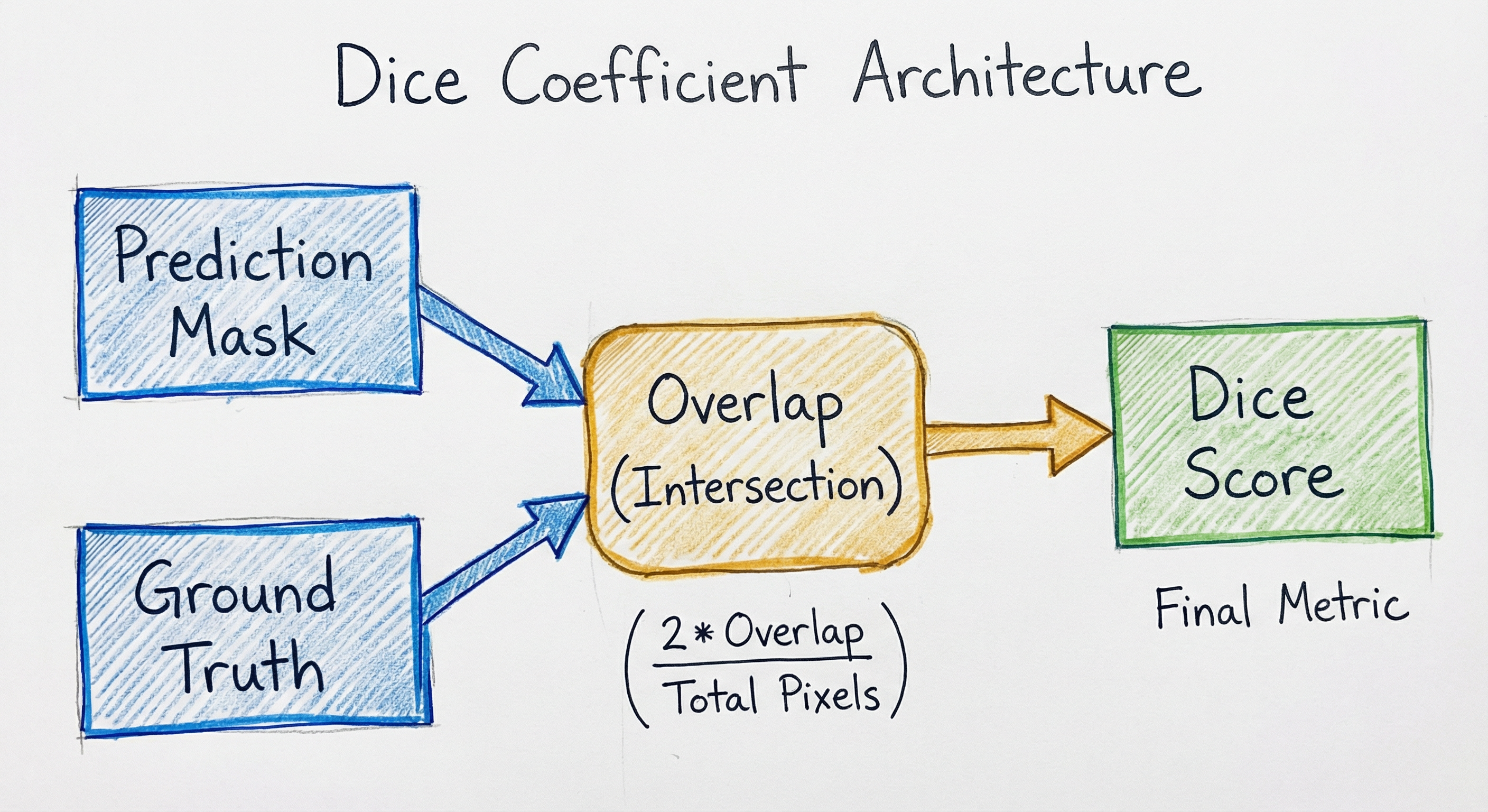
The Dice coefficient (also called the Dice-Sorensen index, or simply Dice score) measures the spatial overlap between a predicted segmentation mask and the ground truth. Its formula is deceptively simple: twice the area of intersection divided by the sum of the two areas. The result is a number between 0 (no overlap) and 1 (perfect agreement). If you recognize this as the harmonic mean of precision and recall applied to pixels, you are exactly right -- the Dice coefficient is the pixel-level F1 score.
But Dice is far more than a metric you compute after training. When turned into a loss function (Dice loss = 1 - Dice), it directly optimizes for segmentation overlap during training. When extended to its "soft" variant, it becomes differentiable and GPU-friendly. When generalized with class weights, it handles the severe class imbalance that plagues real-world segmentation tasks -- where a tumor might occupy 0.5% of the image and background the remaining 99.5%.
From radiology departments in AIIMS Delhi using AI-assisted diagnostic tools to autonomous vehicle teams at Ola Krutrim building road scene parsing, if a system segments anything in an image, the Dice coefficient is likely measuring how well it does that job. Understanding its mechanics, its relationship to IoU, its failure modes, and its many variants is essential for anyone building production segmentation systems.
Concept Snapshot
- What It Is
- A metric that quantifies the overlap between two sets (typically predicted and ground truth segmentation masks) as twice the intersection area divided by the sum of both areas, producing a score from 0 (no overlap) to 1 (perfect match).
- Category
- Evaluation
- Complexity
- Beginner
- Inputs / Outputs
- Inputs: predicted segmentation masks and ground truth masks (binary or multi-class, as pixel arrays or tensors). Outputs: Dice score(s) ranging from 0.0 to 1.0, or mean Dice when averaged across classes.
- System Placement
- Used during model evaluation (offline) to report segmentation quality, and during training (online) as a differentiable loss function (Dice loss). Standard in medical imaging benchmarks, increasingly common in general computer vision.
- Also Known As
- Dice-Sorensen coefficient, Sorensen-Dice index, F1 score (pixel-level), Dice similarity coefficient (DSC), Dice overlap, Samplewise F1
- Typical Users
- Medical imaging researchers, Computer vision engineers, Radiology AI teams, Remote sensing analysts, Autonomous driving perception engineers, ML evaluation engineers
- Prerequisites
- Binary classification (precision, recall, F1), Set theory (intersection, union), Image segmentation fundamentals, Basic calculus (for understanding Dice loss gradients)
- Key Terms
- intersectionsegmentation maskDice losssoft Dicegeneralized Dice lossclass imbalancemean Diceper-class DiceF1 scoreharmonic mean
Why This Concept Exists
The Problem with Pixel Accuracy in Segmentation
When deep learning models began tackling image segmentation in the early 2010s, the obvious evaluation metric was pixel accuracy -- what fraction of pixels were classified correctly? This worked fine for balanced datasets where foreground and background occupied roughly equal area. But real-world segmentation is almost never balanced.
Consider a brain tumor segmentation task. A typical MRI slice might be 256x256 = 65,536 pixels. The tumor might occupy 300 pixels -- less than 0.5% of the image. A model that predicts "no tumor" for every pixel achieves 99.5% pixel accuracy while being completely useless. This is the class imbalance problem, and it made pixel accuracy worthless for practically every medical imaging task.
The Statistician's Solution (1945)
The solution came from an unlikely source. In 1945, American botanist Lee Raymond Dice published a paper introducing a "coefficient of association" to measure the overlap between species ranges in ecology. Independently, in 1948, Danish botanist Thorvald Sorensen proposed an equivalent index for comparing vegetation data. Their formula -- -- turned out to be exactly what medical image segmentation needed half a century later.
The key insight was normalization. Unlike pixel accuracy, Dice normalizes by the sizes of the predicted and ground truth regions themselves (not the entire image). A model that correctly predicts 250 out of 300 tumor pixels, with 50 false positives, gets a Dice score of about 0.83 -- regardless of whether the background is 50,000 or 5,000,000 pixels. The metric "zooms in" on the region of interest.
From Metric to Loss Function
The real breakthrough came when Milletari et al. (2016) proposed using 1 minus the Dice coefficient as a training loss function in their V-Net architecture. This was transformative for two reasons:
- Direct optimization: Instead of training with cross-entropy (a pixel-level surrogate) and evaluating with Dice (a region-level metric), you could now train directly for the metric you care about. This eliminated the misalignment between training objective and evaluation criterion.
- Built-in class balancing: Dice loss inherently handles class imbalance without needing to manually compute class weights or use oversampling. The formula naturally gives equal importance to foreground and background overlap, regardless of their relative sizes.
Sudirman et al. (2019) extended this further with the Generalized Dice Loss, which weights each class by the inverse of its area, providing even stronger handling of multi-class imbalance. Today, Dice loss and its variants are the default training objectives for segmentation in medical imaging, remote sensing, and an increasing share of general computer vision.
Historical Note: The convergence of ecology (Dice, 1945), statistics (Sorensen, 1948), information retrieval (F1 score, van Rijsbergen, 1979), and computer vision (Dice loss, Milletari, 2016) onto the same mathematical formula is remarkable. It suggests that measuring overlap via the harmonic mean of two set-sizes is a fundamentally useful idea that transcends any single domain.
Core Intuition & Mental Model
What Dice Really Measures
Imagine you and a colleague are both asked to outline a tumor on the same MRI scan. You each draw a boundary, creating two regions. The Dice coefficient answers: how similar are your two outlines?
Specifically, it asks: of all the pixels that either of you marked as tumor, what fraction did you both agree on? But it does this with a twist -- it double-counts the agreement (the intersection) to balance between the two reviewers equally.
Here is an intuitive way to think about it. Suppose the tumor is 100 pixels. You marked 90 of the correct tumor pixels plus 20 extra pixels that were actually healthy tissue. Your colleague (ground truth) marked exactly 100 tumor pixels. The intersection (pixels you both agree on) is 90. The Dice score is:
The denominator sums both regions' sizes (your 110 pixels and the ground truth's 100 pixels), which means both missing pixels (false negatives, the 10 tumor pixels you missed) and extra pixels (false positives, the 20 healthy pixels you incorrectly marked) reduce the score. This dual penalty is why Dice is equivalent to the F1 score -- it is the harmonic mean of precision and recall at the pixel level.
Dice vs. IoU: The Sibling Relationship
Dice and IoU are related by a monotonic transformation:
This means they always agree on which of two models is better (rank-preserving), but Dice produces higher numerical scores for the same spatial overlap. A Dice of 0.80 corresponds to an IoU of approximately 0.67. A Dice of 0.90 corresponds to an IoU of approximately 0.82.
Why does this matter? Psychologically, reporting "Dice = 0.90" feels much better than reporting "IoU = 0.82" -- even though they represent identical overlap quality. In medical imaging, where Dice is the convention, this optimism is embraced. In general computer vision benchmarks (COCO, Cityscapes), IoU is preferred because it is stricter and less forgiving.
The "F1 of Pixels" Mental Model
If you already understand precision, recall, and F1 for classification, you understand Dice for segmentation:
- Precision: Of all pixels your model called foreground, what fraction were actually foreground? (i.e., how much of your prediction is correct)
- Recall: Of all actual foreground pixels, what fraction did your model find? (i.e., how much of the ground truth did you capture)
- Dice = F1: The harmonic mean of precision and recall, balancing both concerns equally.
This framing makes it clear why Dice is so popular: it captures the two fundamental failure modes of segmentation (over-segmentation via low precision, under-segmentation via low recall) in a single number.
Technical Foundations
Mathematical Definition
Let be the set of pixels in the predicted segmentation mask and be the set of pixels in the ground truth mask. The Dice coefficient (also called the Dice similarity coefficient, DSC) is defined as:
where denotes the cardinality (number of pixels) of a set and denotes intersection.
Equivalence to F1 Score
For binary segmentation, define:
- True Positives (TP): pixels in both and →
- False Positives (FP): pixels in but not →
- False Negatives (FN): pixels in but not →
Then:
which is exactly the F1 score:
Relationship to IoU (Jaccard Index)
The Dice coefficient and IoU are monotonically related:
Since is strictly increasing for , Dice and IoU always agree on the ranking of models. However, Dice IoU for all overlap values (with equality only at 0 and 1).
Properties
- Bounded:
- Symmetric:
- Identity:
- Null: If and ( or ), then
- Undefined case: If , the formula is . By convention, (perfect agreement on empty).
Soft Dice (Differentiable Version)
For training with gradient descent, we need a differentiable version. Replace binary masks with soft probabilities (model outputs after sigmoid/softmax) and ground truth :
Alternatively (more common in practice):
where is a small smoothing constant (typically to ) that prevents division by zero and provides numerical stability.
Dice Loss
The gradient with respect to predicted probability (for a positive ground truth pixel ) is:
This gradient is always non-zero as long as the prediction is imperfect, which is a significant advantage over IoU loss where the gradient vanishes for non-overlapping regions.
Generalized Dice Loss (GDL)
For multi-class segmentation with severe class imbalance, the Generalized Dice Loss weights each class inversely by its area:
where is the weight for class , inversely proportional to the squared area of that class in the ground truth. This ensures that small structures (e.g., a 50-pixel tumor in a 65,536-pixel image) receive proportionally higher weight in the loss.
Implementation Tip: For binary segmentation, standard Dice loss suffices. For multi-class tasks with imbalanced class sizes (which is almost always the case in medical imaging), use Generalized Dice Loss. For tasks where you need to combine region-level and pixel-level optimization, use a weighted sum of Dice loss and cross-entropy: with .
Internal Architecture
The Dice coefficient is a pure mathematical computation with no trainable parameters. However, in production ML systems, it appears in multiple architectural contexts -- as an evaluation metric, a training loss, and a monitoring signal. Understanding where and how Dice is computed in each context is critical for correct implementation.
The key architectural distinction is between hard Dice (used for evaluation, with thresholded binary masks) and soft Dice (used for training, with continuous probabilities). They produce similar but not identical scores -- soft Dice with a threshold of 0.5 typically slightly exceeds hard Dice because the continuous probabilities encode richer information about prediction confidence.
Key Components
Prediction Processor
Takes raw model outputs (logits) and converts them to either soft probabilities (via sigmoid for binary or softmax for multi-class) for Dice loss computation, or hard masks (via thresholding at 0.5 or argmax) for Dice metric evaluation.
Intersection Calculator
Computes the element-wise product of predicted and ground truth masks (soft Dice: ; hard Dice: ). This is the numerator's core term. Operates per-class for multi-class segmentation.
Area Summation
Computes the sum of predicted mask values () and ground truth mask values () separately. These form the denominator. For the squared variant, computes and instead.
Smoothing & Division
Adds epsilon smoothing to both numerator and denominator to prevent division by zero (especially critical when both prediction and ground truth are empty for a given class). Computes the final Dice score as .
Class Aggregator
For multi-class segmentation, aggregates per-class Dice scores into a single metric. Options include macro-average (mean Dice across all classes), weighted average (weighted by class frequency or inverse frequency), and per-class reporting.
Class Weight Calculator (GDL)
For Generalized Dice Loss, computes per-class weights as the inverse square of the class area in the ground truth batch. This ensures rare classes (small organs, thin boundaries) contribute proportionally to the loss.
Data Flow
Here is how data flows through Dice computation in each context:
During Training (as Dice Loss):
- Model outputs logits of shape (B, C, H, W) for batch size B, C classes, spatial dimensions H x W
- Softmax/sigmoid converts logits to probabilities
- Soft Dice computed per-class:
- Optionally weighted by class (Generalized Dice Loss)
- Loss = 1 - mean(Dice_c), backpropagated through the model
- Often combined with cross-entropy:
During Evaluation (as Metric):
- Model predictions thresholded at 0.5 (binary) or argmax (multi-class) to produce hard masks
- Per-class Dice computed using integer counts (no gradients needed)
- Per-class scores aggregated to mean Dice (macro average)
- Per-class breakdown reported for clinical/domain review
- Results logged to experiment tracker (MLflow, W&B, TensorBoard)
During Annotation Quality Control:
- Multiple annotators segment the same images
- Pairwise Dice computed between annotators per structure
- Low inter-annotator Dice (< 0.75) flags ambiguous cases for expert review
- Mean inter-annotator Dice reported as dataset quality measure
Flow showing model predictions being processed through threshold/argmax and then branching: the evaluation path produces hard Dice scores aggregated into per-class and mean Dice for reporting; the training path computes soft Dice loss that feeds into backpropagation for model weight updates.
How to Implement
Two Implementation Patterns
Dice appears in two distinct implementation contexts:
Pattern 1: Dice as a Metric (Evaluation) Computed on hard (thresholded) binary masks after model inference. No gradients needed. Prioritizes numerical correctness and edge-case handling (empty masks, single-pixel structures). Typically uses NumPy or TorchMetrics.
Pattern 2: Dice as a Loss (Training) Computed on soft (continuous probability) masks during the forward pass. Must be differentiable. Prioritizes GPU efficiency and numerical stability (epsilon smoothing, gradient flow). Always uses PyTorch or TensorFlow tensors.
The critical implementation detail is the smoothing constant epsilon. Without it, when both the prediction and ground truth are empty for a class (e.g., a batch contains no tumors), you get 0/0. The convention is to return 1.0 (perfect agreement that nothing is there), which epsilon naturally handles: .
Cost Note: Dice computation is O(HW) per class per image, where H and W are the spatial dimensions. For a 512x512 image with 5 classes, that is about 1.3M operations -- trivially fast on GPU. A full evaluation of 1,000 medical images takes under a second on a single GPU. In India, a radiology AI startup processing 500 CT scans per day (each with 100-300 slices and 5-10 structures) will compute roughly 750K Dice scores daily. On an NVIDIA T4 GPU (available at approximately 30,000 INR/month or $360/month on AWS Mumbai), this takes seconds.
import numpy as np

def dice_coefficient(pred_mask: np.ndarray, gt_mask: np.ndarray, smooth: float = 1e-6) -> float:
    """
    Compute the Dice coefficient between a predicted binary mask and ground truth.

    Args:
        pred_mask: Binary prediction mask (H, W), values in {0, 1}
        gt_mask: Binary ground truth mask (H, W), values in {0, 1}
        smooth: Smoothing constant to avoid division by zero

    Returns:
        Dice score (float) in [0, 1]
    """
    # Flatten to 1D for simplicity
    pred_flat = pred_mask.flatten().astype(np.float32)
    gt_flat = gt_mask.flatten().astype(np.float32)

    # Intersection: element-wise product (both are binary, so AND = multiply)
    intersection = np.sum(pred_flat * gt_flat)

    # Dice formula: 2 * |A ∩ B| / (|A| + |B|)
    dice = (2.0 * intersection + smooth) / (np.sum(pred_flat) + np.sum(gt_flat) + smooth)

    return float(dice)


def mean_dice_multiclass(pred: np.ndarray, gt: np.ndarray, num_classes: int,
                          ignore_background: bool = True) -> dict:
    """
    Compute per-class and mean Dice for multi-class segmentation.

    Args:
        pred: Predicted class labels (H, W), integer values in [0, num_classes)
        gt: Ground truth class labels (H, W), integer values in [0, num_classes)
        num_classes: Total number of classes (including background)
        ignore_background: If True, exclude class 0 from mean Dice

    Returns:
        Dict with 'per_class' (list of per-class Dice) and 'mean' (mean Dice)
    """
    per_class_dice = []
    start_class = 1 if ignore_background else 0

    for c in range(start_class, num_classes):
        pred_c = (pred == c).astype(np.float32)
        gt_c = (gt == c).astype(np.float32)
        dice_c = dice_coefficient(pred_c, gt_c)
        per_class_dice.append(dice_c)

    return {
        'per_class': per_class_dice,
        'mean': float(np.mean(per_class_dice)) if per_class_dice else 0.0
    }


# Example usage
np.random.seed(42)
gt = np.zeros((256, 256), dtype=np.uint8)
gt[80:180, 80:180] = 1  # 100x100 square tumor

pred = np.zeros((256, 256), dtype=np.uint8)
pred[85:175, 85:175] = 1  # Slightly smaller prediction

dice = dice_coefficient(pred, gt)
print(f"Dice coefficient: {dice:.4f}")
# Dice coefficient: 0.9121
This is the canonical Dice implementation for binary and multi-class segmentation. The key steps: (1) flatten masks, (2) compute intersection as element-wise product and sum, (3) apply the Dice formula with epsilon smoothing. The multi-class version treats each class as a binary problem (one-vs-rest) and averages. The ignore_background option is important -- in medical imaging, background Dice is almost always near 1.0 (trivially easy) and inflates the mean, so it is typically excluded.
import torch
import torch.nn as nn
import torch.nn.functional as F

class SoftDiceLoss(nn.Module):
    """
    Soft Dice Loss for binary or multi-class segmentation.

    Uses soft probabilities (no thresholding) to maintain differentiability.
    Supports per-class computation and optional background exclusion.
    """

    def __init__(self, smooth: float = 1e-6, ignore_background: bool = True):
        super().__init__()
        self.smooth = smooth
        self.ignore_background = ignore_background

    def forward(self, logits: torch.Tensor, targets: torch.Tensor) -> torch.Tensor:
        """
        Args:
            logits: Model output, shape (B, C, H, W) for C classes
            targets: Ground truth class indices, shape (B, H, W), values in [0, C)

        Returns:
            Scalar Dice loss
        """
        num_classes = logits.shape[1]

        # Convert logits to probabilities
        probs = F.softmax(logits, dim=1)  # (B, C, H, W)

        # One-hot encode targets: (B, H, W) -> (B, C, H, W)
        targets_onehot = F.one_hot(targets.long(), num_classes)  # (B, H, W, C)
        targets_onehot = targets_onehot.permute(0, 3, 1, 2).float()  # (B, C, H, W)

        # Determine which classes to include
        start_class = 1 if self.ignore_background else 0

        # Compute per-class Dice
        dice_scores = []
        for c in range(start_class, num_classes):
            p = probs[:, c]          # (B, H, W)
            g = targets_onehot[:, c]  # (B, H, W)

            # Flatten spatial dimensions
            p_flat = p.reshape(p.shape[0], -1)  # (B, H*W)
            g_flat = g.reshape(g.shape[0], -1)  # (B, H*W)

            # Soft Dice per sample in batch
            intersection = (p_flat * g_flat).sum(dim=1)  # (B,)
            union = p_flat.sum(dim=1) + g_flat.sum(dim=1)  # (B,)

            dice_c = (2.0 * intersection + self.smooth) / (union + self.smooth)  # (B,)
            dice_scores.append(dice_c.mean())  # Average over batch

        # Average over classes
        mean_dice = torch.stack(dice_scores).mean()

        return 1.0 - mean_dice


# Example: training loop snippet
model = torch.nn.Conv2d(3, 5, kernel_size=3, padding=1)  # Toy model, 5 classes
criterion = SoftDiceLoss(smooth=1e-6, ignore_background=True)
optimizer = torch.optim.Adam(model.parameters(), lr=1e-3)

# Simulated batch
images = torch.randn(4, 3, 128, 128)  # 4 images, 3 channels, 128x128
targets = torch.randint(0, 5, (4, 128, 128))  # Random class labels

# Forward pass
logits = model(images)
loss = criterion(logits, targets)
loss.backward()
optimizer.step()
print(f"Dice loss: {loss.item():.4f}")
This soft Dice loss implementation is differentiable and GPU-friendly. Key design decisions: (1) softmax on logits to get probabilities (not sigmoid, since this is multi-class), (2) one-hot encoding of targets for per-class computation, (3) epsilon smoothing in both numerator and denominator, (4) per-sample Dice within the batch, then averaged. The ignore_background flag excludes the trivially easy background class from the loss, forcing the model to focus on foreground structures.
import torch
import torch.nn as nn
import torch.nn.functional as F

class GeneralizedDiceLoss(nn.Module):
    """
    Generalized Dice Loss (GDL) for multi-class segmentation with
    severe class imbalance.

    Weights each class by the inverse square of its ground truth area,
    ensuring small structures (e.g., tumors, thin boundaries) contribute
    proportionally to the loss.

    Reference: Sudre et al., "Generalised Dice overlap as a deep learning
    loss function for highly unbalanced segmentations", DLMIA 2017.
    """

    def __init__(self, smooth: float = 1e-6, weight_type: str = 'square'):
        super().__init__()
        self.smooth = smooth
        self.weight_type = weight_type  # 'square', 'simple', or 'uniform'

    def forward(self, logits: torch.Tensor, targets: torch.Tensor) -> torch.Tensor:
        """
        Args:
            logits: (B, C, H, W) model output logits
            targets: (B, H, W) ground truth class indices

        Returns:
            Scalar generalized Dice loss
        """
        num_classes = logits.shape[1]
        probs = F.softmax(logits, dim=1)  # (B, C, H, W)

        # One-hot encode targets
        targets_onehot = F.one_hot(targets.long(), num_classes)  # (B, H, W, C)
        targets_onehot = targets_onehot.permute(0, 3, 1, 2).float()  # (B, C, H, W)

        # Flatten spatial dimensions
        probs_flat = probs.reshape(probs.shape[0], num_classes, -1)      # (B, C, N)
        targets_flat = targets_onehot.reshape(probs.shape[0], num_classes, -1)  # (B, C, N)

        # Per-class ground truth areas for weighting
        class_areas = targets_flat.sum(dim=2)  # (B, C)

        # Compute class weights
        if self.weight_type == 'square':
            weights = 1.0 / (class_areas ** 2 + self.smooth)  # (B, C)
        elif self.weight_type == 'simple':
            weights = 1.0 / (class_areas + self.smooth)
        else:
            weights = torch.ones_like(class_areas)  # Uniform

        # Weighted intersection and union
        intersection = (probs_flat * targets_flat).sum(dim=2)  # (B, C)
        union = probs_flat.sum(dim=2) + targets_flat.sum(dim=2)  # (B, C)

        # Generalized Dice
        weighted_inter = (weights * intersection).sum(dim=1)  # (B,)
        weighted_union = (weights * union).sum(dim=1)  # (B,)

        gdl = 1.0 - (2.0 * weighted_inter + self.smooth) / (weighted_union + self.smooth)

        return gdl.mean()


# Example: brain tumor segmentation (4 classes: background, tumor core,
# enhancing tumor, edema -- with severe imbalance)
model = torch.nn.Conv2d(4, 4, kernel_size=3, padding=1)  # 4-channel MRI, 4 classes
criterion = GeneralizedDiceLoss(smooth=1e-6, weight_type='square')

images = torch.randn(2, 4, 240, 240)  # 2 BraTS-style images
targets = torch.zeros(2, 240, 240, dtype=torch.long)  # Mostly background
targets[:, 100:140, 100:140] = 1  # Small tumor core (40x40)
targets[:, 105:135, 105:135] = 2  # Even smaller enhancing tumor (30x30)
targets[:, 90:150, 90:150] = 3    # Larger edema (60x60)
targets[:, 100:140, 100:140] = 1  # Re-stamp tumor core

logits = model(images)
loss = criterion(logits, targets)
print(f"Generalized Dice Loss: {loss.item():.4f}")
Generalized Dice Loss addresses the core weakness of standard Dice loss in multi-class settings: if one class dominates (e.g., background = 95% of pixels), standard Dice loss is overwhelmed by that class. GDL weights each class inversely by its area squared, so a 50-pixel tumor contributes as much to the loss as a 50,000-pixel background. The weight_type='square' option (inverse square weighting) is the original formulation from Sudre et al. and is the most commonly used. This is the default loss for BraTS (brain tumor segmentation challenge) and most medical imaging competitions.
import torch
import torch.nn as nn
import torch.nn.functional as F

class DiceCELoss(nn.Module):
    """
    Combined Dice Loss + Cross-Entropy Loss.

    Dice provides region-level optimization (overlap quality).
    Cross-entropy provides pixel-level optimization (calibrated probabilities).
    Together they produce better-calibrated, more stable training than either alone.

    This is the default loss in nnU-Net, the top-performing medical segmentation
    framework, and is widely considered best practice.
    """

    def __init__(self, dice_weight: float = 0.5, ce_weight: float = 0.5,
                 smooth: float = 1e-6, ignore_index: int = -100):
        super().__init__()
        self.dice_weight = dice_weight
        self.ce_weight = ce_weight
        self.smooth = smooth
        self.ce_loss = nn.CrossEntropyLoss(ignore_index=ignore_index)

    def dice_loss(self, logits: torch.Tensor, targets: torch.Tensor) -> torch.Tensor:
        num_classes = logits.shape[1]
        probs = F.softmax(logits, dim=1)
        targets_onehot = F.one_hot(targets.long(), num_classes).permute(0, 3, 1, 2).float()

        # Per-class Dice (skip background)
        dice_scores = []
        for c in range(1, num_classes):
            p = probs[:, c].reshape(probs.shape[0], -1)
            g = targets_onehot[:, c].reshape(probs.shape[0], -1)
            inter = (p * g).sum(dim=1)
            total = p.sum(dim=1) + g.sum(dim=1)
            dice_c = (2.0 * inter + self.smooth) / (total + self.smooth)
            dice_scores.append(dice_c.mean())

        return 1.0 - torch.stack(dice_scores).mean()

    def forward(self, logits: torch.Tensor, targets: torch.Tensor) -> torch.Tensor:
        d_loss = self.dice_loss(logits, targets)
        c_loss = self.ce_loss(logits, targets)
        return self.dice_weight * d_loss + self.ce_weight * c_loss


# nnU-Net style training
criterion = DiceCELoss(dice_weight=0.5, ce_weight=0.5)
logits = torch.randn(4, 3, 128, 128)  # 4 images, 3 classes
targets = torch.randint(0, 3, (4, 128, 128))

loss = criterion(logits, targets)
print(f"Combined Dice+CE Loss: {loss.item():.4f}")
The Dice + cross-entropy combination is the most widely used loss for segmentation. Dice loss alone can produce poorly calibrated probabilities (overconfident predictions) because it does not directly penalize individual pixel confidence. Cross-entropy alone struggles with class imbalance. Together, Dice handles the imbalance and optimizes overlap, while CE ensures pixel-level gradient signal and probability calibration. This exact combination (with equal weights) is the default in nnU-Net, which has won or topped the leaderboard in virtually every medical segmentation challenge since 2018.
# TorchMetrics configuration for multi-class segmentation
from torchmetrics.segmentation import Dice

dice_metric = Dice(
    num_classes=4,              # Number of classes including background
    average='macro',            # Macro average (per-class, then mean)
    ignore_index=0,             # Ignore background class in mean
    zero_division=1.0,          # Return 1.0 when both pred and gt are empty
    input_format='index',       # Input is class indices, not one-hot
    multidim_average='global',  # Global average across spatial dims
)

# MONAI configuration for medical imaging
from monai.metrics import DiceMetric

dice_metric = DiceMetric(
    include_background=False,    # Exclude background from mean
    reduction='mean_batch',      # Average over batch, per-class results
    get_not_nans=True,          # Track NaN counts for empty classes
    ignore_empty=True,          # Handle empty predictions/GTs
)

# nnU-Net default loss configuration
from nnunetv2.training.loss.dice import SoftDiceLoss
from nnunetv2.training.loss.compound_losses import DC_and_CE_loss

loss = DC_and_CE_loss(
    soft_dice_kwargs={'batch_dice': False, 'smooth': 1e-5, 'do_bg': False},
    ce_kwargs={},
    weight_ce=1.0,
    weight_dice=1.0,
)
Common Implementation Mistakes
- ●
Forgetting epsilon smoothing when both prediction and ground truth are empty for a class. Without smoothing, you get 0/0 = NaN, which corrupts the loss and can crash training. Always add epsilon (1e-6) to both numerator and denominator. Some implementations add epsilon only to the denominator, but adding to both ensures the Dice score approaches 1.0 (correct behavior) when both sets are empty.
- ●
Computing Dice on soft probabilities during evaluation (instead of hard masks). Soft Dice scores are typically higher than hard Dice scores because continuous probabilities encode more overlap information. For reporting and comparison with published results, always threshold predictions first (0.5 for binary, argmax for multi-class) and compute hard Dice. Use soft Dice only during training.
- ●
Not handling the per-sample vs. per-batch computation correctly. Dice should be computed per sample (image) in the batch and then averaged, NOT computed on the concatenation of all samples. Computing batch-level Dice allows large images to dominate and produces different gradients than per-sample Dice, leading to inconsistent training behavior.
- ●
Including background class in mean Dice for medical segmentation. Background typically occupies 90-99% of the image and achieves Dice > 0.99 trivially. Including it inflates mean Dice and masks poor performance on foreground structures. Always report mean Dice with background excluded (this is the convention in BraTS, ACDC, and most medical benchmarks).
- ●
Using standard Dice loss for multi-class segmentation with severe imbalance without class weighting. If one class is 1000x larger than another, standard Dice loss barely penalizes errors on the small class. Use Generalized Dice Loss or the Dice+CE combination. Alternatively, compute Dice loss per class and weight by inverse class frequency.
- ●
Comparing Dice scores across papers without checking thresholding and post-processing. A Dice of 0.85 with CRF post-processing is not the same as 0.85 without post-processing. Always specify: (1) hard vs. soft Dice, (2) threshold used, (3) whether post-processing was applied, (4) whether background is included in the mean.
When Should You Use This?
Use When
Evaluating segmentation models in medical imaging (brain tumor, organ, lesion segmentation) where Dice is the established standard metric used in challenges like BraTS, ACDC, KiTS, and most clinical studies
Training segmentation models on severely imbalanced datasets where foreground structures occupy less than 5% of the image area, and pixel-level losses like cross-entropy fail to produce useful gradients for the minority class
You need a metric that is equivalent to the F1 score at the pixel level, providing a balanced view of both precision (how much of your prediction is correct) and recall (how much of the ground truth you captured)
Comparing segmentation quality across models or configurations where you need a normalized, interpretable score between 0 and 1 that is independent of image size or class distribution
You need a differentiable training loss that directly optimizes for overlap quality rather than pixel-wise surrogate objectives, and you want built-in class imbalance handling without manual weight tuning
Evaluating inter-annotator agreement for segmentation annotations, where Dice provides a straightforward measure of how consistently different annotators delineate the same structure
Avoid When
Evaluating object detection (bounding box predictions) -- IoU and mAP are the established metrics; Dice is not used for box overlap in standard benchmarks
Your segmentation task has equally important boundary precision -- Dice measures area overlap but is insensitive to boundary details; use Hausdorff distance or surface Dice alongside Dice for boundary-critical tasks
You need to rank models on general computer vision benchmarks (COCO, Cityscapes) -- these benchmarks use IoU/mIoU, not Dice, and using Dice would make your results incomparable
The segmentation outputs require probability calibration -- Dice loss alone produces poorly calibrated probabilities; combine with cross-entropy or use temperature scaling post-hoc
You are evaluating panoptic segmentation where you need to jointly evaluate recognition and segmentation quality -- use Panoptic Quality (PQ), which combines recognition IoU with segmentation IoU
The predicted regions are non-spatial (e.g., text classification, tabular data) -- use standard F1 score instead; Dice is only meaningful for spatial overlap
Key Tradeoffs
Dice vs. IoU: The Core Choice
Dice and IoU are the two primary segmentation metrics, and the choice between them is largely driven by convention:
| Aspect | Dice | IoU |
|---|---|---|
| Score range | 0-1 (higher for same overlap) | 0-1 (lower for same overlap) |
| Convention | Medical imaging, BraTS, ISBI | COCO, Cityscapes, PASCAL VOC |
| Imbalance handling | Slightly more robust | More sensitive to small errors on tiny objects |
| Loss function | Widely used (Dice loss) | Used but gradient vanishes at 0 overlap |
| Psychology | "Optimistic" scores | "Realistic" scores |
For the same spatial overlap, Dice always produces a higher score than IoU (except at 0 and 1). This is not a mathematical advantage -- it is simply a different scale. However, the practical impact is real: stakeholders (clinicians, product managers) respond better to "Dice = 0.90" than "IoU = 0.82," even though they describe identical performance.
Dice Loss vs. Cross-Entropy: Complementary, Not Competing
Dice loss optimizes at the region level (entire foreground vs. background overlap), while cross-entropy optimizes at the pixel level (each pixel independently). Neither is strictly better:
- Dice loss alone: Great for imbalanced data, but can produce poorly calibrated probabilities and sometimes leads to training instability (oscillating loss). Tends to produce "blobby" predictions with smooth boundaries.
- Cross-entropy alone: Provides stable pixel-level gradients and well-calibrated probabilities, but is dominated by the majority class in imbalanced settings. Requires explicit class weighting.
- Dice + CE (best practice): Combines the strengths of both. Dice handles imbalance and overlap optimization; CE provides stable gradients and calibration. This is the nnU-Net default and is recommended for almost all segmentation tasks.
Cost Considerations for Indian Teams
Dice computation is extremely cheap. The real cost is in the segmentation model itself:
| Resource | Cost (India / AWS Mumbai) |
|---|---|
| NVIDIA T4 (16GB) for training | ~30,000 INR/month ($360) |
| NVIDIA A10G (24GB) for training | ~60,000 INR/month ($720) |
| Dice evaluation on 1000 images | < 1 second on T4 |
| Dice loss computation per batch | < 1ms on T4 |
The bottleneck is always model inference, not Dice computation. Invest in optimizing model architecture (U-Net vs. SegFormer vs. nnU-Net), not Dice implementation.
Rule of Thumb: Use Dice for medical imaging, IoU for general CV, and report both when your audience spans domains. For training, use Dice+CE unless you have a specific reason not to.
Alternatives & Comparisons
IoU and Dice are monotonically related (Dice = 2*IoU/(1+IoU)) and always agree on model ranking. IoU is stricter (lower scores for the same overlap), making it the convention in general computer vision benchmarks (COCO, Cityscapes, PASCAL VOC). Dice is more forgiving and is the convention in medical imaging. Choose Dice for medical imaging or when communicating to non-technical stakeholders (higher scores are psychologically easier). Choose IoU when publishing on standard CV benchmarks. When in doubt, report both.
The Dice coefficient IS the F1 score applied at the pixel level. The advantage of reporting Dice (rather than precision and recall separately) is its single-number simplicity. However, when you need to distinguish between over-segmentation (low precision) and under-segmentation (low recall), reporting precision and recall separately alongside Dice gives a more complete picture. For tasks where false positives and false negatives have very different costs, prefer precision/recall with task-appropriate thresholds over the balanced Dice.
mAP is used for object detection and instance segmentation (per-instance evaluation), while Dice is used for semantic segmentation (per-pixel evaluation). They serve different tasks and are not directly comparable. For instance segmentation, COCO uses mask IoU within its mAP computation. Dice is not used in the mAP framework. If you are doing instance segmentation, use mAP; if semantic segmentation, use Dice or mIoU.
PSNR and SSIM measure image reconstruction quality (how similar two images look), while Dice measures segmentation overlap (how well two binary/labeled regions match). They are used for fundamentally different tasks -- PSNR/SSIM for super-resolution, denoising, and image generation; Dice for segmentation. The only overlap is in medical image reconstruction pipelines where a reconstructed image is then segmented and the segmentation is evaluated with Dice.
Pros, Cons & Tradeoffs
Advantages
Inherently handles class imbalance by normalizing against the sizes of the predicted and ground truth regions rather than the entire image. A tiny tumor in a huge image gets a meaningful score without manual class weighting, unlike pixel accuracy or unweighted cross-entropy.
Equivalent to F1 score at the pixel level, giving a balanced measure of precision (how much of the prediction is correct) and recall (how much of the ground truth is captured). This dual-penalty property makes it informative about both over-segmentation and under-segmentation.
Directly usable as a training loss (Dice loss) that aligns the optimization objective with the evaluation metric. This eliminates the training-evaluation gap that exists when training with cross-entropy but evaluating with Dice or IoU.
Numerically higher than IoU for the same spatial overlap, which makes it psychologically easier to communicate to non-technical stakeholders (clinicians, product managers). Dice = 0.90 sounds better than IoU = 0.82, even though they describe identical quality.
Generalized Dice Loss (GDL) extends Dice to multi-class settings with built-in per-class weighting, handling extreme imbalance (e.g., 4+ classes where the smallest occupies < 0.1% of pixels) without manual weight tuning.
Simple to implement (5-10 lines of NumPy) yet available in production-ready form in all major frameworks (PyTorch, TensorFlow, MONAI, TorchMetrics). Easy to prototype and scale.
Well-established standard in medical imaging, with decades of published results enabling direct comparison. If you are building a medical AI system, Dice is the metric your reviewers, regulators, and collaborators expect.
Disadvantages
Insensitive to boundary quality. Dice measures area overlap, not boundary alignment. Two predictions with identical Dice can have very different boundary precision -- one might be smooth and accurate, the other jagged and noisy. For boundary-critical tasks (e.g., surgical planning), supplement Dice with Hausdorff distance or surface Dice.
Dice loss alone produces poorly calibrated probabilities. Because Dice loss operates at the region level, it does not directly penalize overconfident incorrect pixels. Models trained with only Dice loss tend to produce sharper but less calibrated probability maps. Always combine with cross-entropy for production use.
Sensitive to small prediction volumes. For very small structures (< 20 pixels), a few-pixel error causes dramatic Dice swings. A prediction that misses 5 pixels out of 15 drops from Dice ~0.67 to ~0.50, while missing 5 out of 1500 barely changes the score. This makes Dice unreliable for evaluating tiny structures.
The "optimistic" scoring can mask poor performance. Dice = 0.75 might sound acceptable, but it corresponds to IoU = 0.60, which means 40% of the combined region is incorrectly segmented. Teams unfamiliar with the Dice-IoU relationship may overestimate model quality.
Training instability with pure Dice loss. Dice loss gradients depend on the global prediction statistics (total foreground pixels), which can change dramatically between batches. This can cause oscillating loss curves and slower convergence compared to cross-entropy. Mitigated by combining with CE.
Not suitable for object detection or instance-level evaluation. Dice treats the entire prediction as one region; it cannot distinguish between two separate tumor instances or count objects. For instance segmentation, use mAP with mask IoU.
Convention-dependent interpretation. A Dice score of 0.85 means different things in different contexts (organ segmentation vs. lesion segmentation vs. cell segmentation). Always report the task, dataset, and whether background is included.
Failure Modes & Debugging
Catastrophic failure on tiny structures
Cause
When the ground truth structure is very small (< 30 pixels), even a minor misalignment of 3-5 pixels causes the intersection to drop dramatically relative to the small total areas. The Dice score becomes extremely volatile -- a single pixel can swing the score by 0.05-0.10.
Symptoms
High variance in per-structure Dice scores for small objects. Mean Dice across patients looks acceptable, but individual small lesions show Dice ranging from 0.2 to 0.9 despite visually similar segmentation quality. Clinicians report inconsistent AI performance on small findings.
Mitigation
Report Dice stratified by structure size (small/medium/large). For tiny structures, supplement Dice with detection-based metrics (was the structure found at all?) and boundary metrics (Hausdorff distance, surface Dice). Consider the Tversky loss with alpha < 0.5 to reduce false negative penalty for small structures. In clinical settings, a Dice threshold of 0.5 (rather than 0.7) may be appropriate for structures under 100 pixels.
Mean Dice masking per-class failures
Cause
Mean Dice averages across all classes equally. If the model excels on 3 out of 4 classes (Dice > 0.90) but completely fails on the 4th class (Dice < 0.30), the mean Dice is still 0.75 -- which looks acceptable. This is especially dangerous when the failing class is clinically critical (e.g., enhancing tumor in BraTS).
Symptoms
Mean Dice meets the deployment threshold, but post-deployment clinical review reveals the model consistently misses one structure type. Per-class Dice inspection would have caught this before deployment. The issue is amplified when background is accidentally included in the mean.
Mitigation
Always report per-class Dice alongside mean Dice. Set minimum per-class thresholds as deployment gates -- do not deploy if ANY critical class falls below its threshold, regardless of the mean. Use Generalized Dice Loss during training to ensure the model does not neglect rare classes. Create dashboards that highlight the worst-performing class prominently.
Training instability with pure Dice loss
Cause
Dice loss gradients depend on the ratio of intersection to total area across the entire image. When predictions change significantly between iterations (common early in training), this ratio oscillates, causing unstable gradients. The problem is worse with small batch sizes (each batch has different class distributions) and highly imbalanced data (small foreground means the denominator is sensitive to prediction changes).
Symptoms
Loss curve oscillates wildly instead of decreasing smoothly. Training Dice score fluctuates by 0.1-0.2 between consecutive epochs. Model predictions alternate between over-segmentation and under-segmentation rather than converging. In extreme cases, training diverges entirely.
Mitigation
Combine Dice loss with cross-entropy (50/50 or 30/70 Dice/CE weighting). The CE component provides stable per-pixel gradients that anchor training while Dice handles overlap optimization. Use larger batch sizes (8+ for 2D, 2+ for 3D) to stabilize class distribution statistics within each batch. Apply gradient clipping (max norm 1.0) to prevent explosion. The nnU-Net default (Dice + CE with batch size 2-5) is a proven stable configuration.
Overconfident predictions from Dice-only training
Cause
Dice loss optimizes the region-level overlap without penalizing the confidence of individual pixel predictions. A model can achieve high Dice by producing sharp (0/1) predictions that are correct on average, even if individual borderline pixels are overconfident. This happens because Dice loss does not include a calibration term.
Symptoms
Model predictions are binary-looking (very few pixels with intermediate probabilities). Soft Dice during training is much higher than hard Dice during evaluation. Reliability diagrams show overconfidence -- the model predicts 0.95 probability for pixels that are actually correct only 70% of the time. Downstream uncertainty-based workflows (e.g., flagging uncertain predictions for human review) fail because the model expresses no uncertainty.
Mitigation
Add cross-entropy to the loss (). Apply temperature scaling post-hoc to calibrate probabilities. If using predictions for uncertainty estimation, train with an explicit calibration objective (e.g., focal loss) alongside Dice. Report Expected Calibration Error (ECE) alongside Dice to monitor calibration.
Inconsistent evaluation due to post-processing variations
Cause
Dice scores are highly sensitive to post-processing choices: connected component filtering, morphological operations (opening, closing), conditional random fields (CRFs), and test-time augmentation (TTA). Two teams might achieve 0.87 and 0.85 Dice with identical models but different post-processing, and declare different winners. Challenge submissions often achieve 2-5% Dice improvement from post-processing alone.
Symptoms
Dice scores jump by 3-5% when post-processing is added. Published results are not reproducible when the post-processing pipeline differs. Internal ablation studies show larger effects from post-processing hyperparameters (e.g., minimum connected component size) than from model architecture changes.
Mitigation
Always report Dice both with and without post-processing so the model's intrinsic capability is clear. Standardize post-processing in team protocols and document every step. When comparing with published results, check whether their Dice includes post-processing. For challenges, follow the organizer's evaluation protocol exactly. Use MONAI's compute_dice with standardized settings for reproducibility.
Epsilon sensitivity in edge cases
Cause
The smoothing constant epsilon affects Dice scores when either the prediction or ground truth is very small. A large epsilon (e.g., 1.0) inflates Dice scores for small structures, while a very small epsilon (e.g., 1e-10) can cause numerical instability. Different implementations use different epsilon values, leading to subtly different scores.
Symptoms
Dice scores differ by 0.01-0.03 between different evaluation libraries for the same predictions. Empty-class handling varies -- some return 0.0, others 1.0, and still others NaN. Reproducibility issues when migrating between frameworks (TorchMetrics vs. MONAI vs. custom code).
Mitigation
Standardize epsilon across your codebase (1e-5 to 1e-7 is the typical range; 1e-6 is a safe default). Explicitly handle the empty-set case: if both prediction and ground truth are empty for a class, return 1.0 (correct agreement). If only one is empty, return 0.0 (complete disagreement). Document your epsilon and empty-set convention in model cards and evaluation reports.
Placement in an ML System
Where Dice Sits in the ML Pipeline
Dice appears at three stages in the lifecycle of a segmentation system:
During Training (as a Loss Function) Dice loss (or its variants: Generalized Dice, Dice+CE) is computed on every forward pass. The model outputs class probabilities for each pixel, soft Dice is computed against the ground truth, and the gradient is backpropagated. This runs thousands of times per epoch. Dice loss is almost always the primary (or co-primary) loss function for segmentation, especially in medical imaging.
During Evaluation (as a Metric) After training, model predictions are thresholded (binary) or argmaxed (multi-class) and hard Dice is computed against held-out test data. Per-class and mean Dice are reported. This is the number that appears in papers, regulatory submissions, and deployment decisions. In challenges like BraTS, Dice scores are computed on a held-out test set by the organizers using standardized evaluation code.
Post-Deployment (for Monitoring) In production systems where a subset of predictions are reviewed by human experts (e.g., a radiologist reviews 10% of AI segmentations), Dice is computed between the AI output and the expert correction. Trends in this Dice score over time detect performance drift. A drop from 0.88 to 0.82 over three months might indicate distribution shift (new scanner hardware, different patient population).
Key Insight: Dice unifies training and evaluation in a way that cross-entropy cannot. When you train with Dice loss and evaluate with Dice metric, the model directly optimizes for the number you report. This alignment is why Dice-based training dominates medical image segmentation.
Pipeline Stage
Evaluation & Training
Upstream
- segmentation
- image-preprocessor
- Annotation Pipeline
- Model Training Loop
Downstream
- Model Registry (deployment gate)
- Monitoring Dashboard
- Clinical Reporting
- Model Comparison Reports
Scaling Bottlenecks
Dice computation itself is cheap (O(HW) per class per image), but it appears in contexts where scale considerations matter:
1. 3D Medical Imaging For volumetric data (CT/MRI), a single volume might be 512x512x300 = 78M voxels. With 5 classes, that is 390M comparisons per volume. A validation set of 100 volumes requires 39 billion comparisons. On a single GPU, this takes 30-60 seconds. For real-time clinical deployment (processing a scan while the patient waits), Dice evaluation must be optimized with float16 operations and multi-GPU parallelism.
2. Training with Dice Loss on Large Batches Dice loss requires computing sums across all spatial positions per class per sample. For 3D segmentation with large patches (128x128x128), this is 2M voxels per sample. The softmax and one-hot encoding create temporary tensors that consume GPU memory: a batch of 4 images with 10 classes at 128x128x128 requires ~4GB just for the Dice loss computation tensors. Memory-efficient implementations (in-place operations, gradient checkpointing) are essential for large 3D models.
3. Annotation Quality at Scale A large medical imaging dataset (e.g., 50,000 studies with 3 annotators each) requires 150K pairwise Dice computations for quality control. This is trivially parallelizable but needs infrastructure (batch processing, result aggregation) to run efficiently.
- Memory for 3D volumes: Use patch-based evaluation (compute Dice on overlapping patches and aggregate) rather than loading entire volumes into GPU memory. MONAI provides
sliding_window_inferencefor this. - Multi-GPU evaluation: Distribute volumes across GPUs and aggregate per-class statistics (TP, FP, FN) before computing final Dice. TorchMetrics handles this with
dist_sync_on_step. - I/O bottleneck: For large datasets stored on disk, data loading (NIfTI/DICOM files) is often slower than Dice computation. Use pre-cached tensor formats (HDF5, zarr) and parallel data loaders.
Production Case Studies
nnU-Net is the self-configuring segmentation framework that has won or placed top-3 in virtually every major medical imaging challenge since 2018 (BraTS, KiTS, ACDC, MSD, and dozens more). Its default loss function is Dice + cross-entropy (50/50 weighting), and it evaluates using per-class Dice with background excluded. The framework automatically configures all hyperparameters (patch size, architecture depth, augmentation) based on dataset properties, but the Dice+CE loss is fixed as a proven universal default. nnU-Net demonstrated that a well-tuned U-Net with Dice+CE loss outperforms specialized architectures (attention U-Net, TransUNet) on most segmentation tasks.
Mean Dice scores of 0.87-0.93 across diverse tasks (brain tumor, kidney tumor, cardiac, liver, pancreas segmentation). The Dice+CE loss was shown to be strictly better than either Dice or CE alone across all 10 tasks in the Medical Segmentation Decathlon. Cited in 3000+ papers and used as the baseline in most medical segmentation research.
Predible Health, a Bengaluru-based healthcare AI startup (now part of Tricog Health), developed AI-powered CT scan analysis tools for lung nodule detection and liver lesion segmentation. Their segmentation models are evaluated using per-structure Dice scores, with clinical validation requiring Dice > 0.80 for liver segmentation and > 0.70 for lung nodule delineation. They use Generalized Dice Loss during training to handle the severe imbalance between lesion and healthy tissue. The system is deployed across 100+ hospitals in India, processing scans at a cost of approximately 200-500 INR (6) per scan, compared to 2,000-5,000 INR (60) for manual radiologist annotation.
Achieved mean Dice of 0.84 for liver segmentation and 0.76 for lung nodule segmentation on internal validation. Processing time under 30 seconds per scan on cloud GPUs (AWS Mumbai region). The AI system reduced radiologist reporting time by 40% on average, with Dice-based quality monitoring ensuring consistent performance across hospital sites.
While AlphaFold is primarily known for protein structure prediction, the team's work on medical image segmentation for retinal OCT scans (diabetic retinopathy, age-related macular degeneration) uses Dice as the primary evaluation metric. Their DeepMind Health division published results on segmenting retinal layers and fluid regions, achieving Dice scores that matched or exceeded expert ophthalmologists. The system was clinically validated at Moorfields Eye Hospital (London) with Dice-based comparison between AI and expert annotations.
Mean Dice of 0.91 for retinal layer segmentation across 9 tissue classes, matching the inter-expert Dice of 0.90. The AI recommendations matched clinical expert referral decisions 94% of the time. This work demonstrated that Dice-based evaluation can bridge the gap between AI performance metrics and clinical acceptance criteria.
Airbus sponsored a major Kaggle competition for ship detection and segmentation in satellite imagery, using Dice as the primary evaluation metric. Participants needed to segment ship pixels in high-resolution satellite images where ships might occupy less than 0.1% of the image area -- an extreme class imbalance scenario. The winning solutions used Dice loss combined with focal loss during training, with post-processing to separate overlapping ship instances. The competition demonstrated that Dice is effective even for extremely sparse segmentation targets when combined with appropriate training strategies.
Top solutions achieved Dice scores of 0.85+ on the private leaderboard. The competition attracted 884 teams and demonstrated that Dice-based evaluation works well for industrial remote sensing applications. Key insight: combining Dice loss with instance-aware post-processing was critical for separating adjacent ships.
Tooling & Ecosystem
The leading open-source framework for medical image segmentation, developed by NVIDIA and King's College London. Provides DiceMetric, DiceLoss, GeneralizedDiceLoss, DiceCELoss, and DiceFocalLoss with production-ready implementations. Handles 2D and 3D data natively, supports distributed evaluation, and includes the compute_dice utility for standard evaluation. MONAI's Dice implementations are the de facto standard for medical imaging research and are used by most top-performing submissions in medical segmentation challenges.
Production-ready metrics library for PyTorch with an optimized Dice metric class supporting multi-class, multi-label, micro/macro/weighted averaging, and distributed GPU computation. Integrates seamlessly with PyTorch Lightning for automatic metric logging during training and validation. Handles edge cases (empty predictions, empty ground truth) and provides both functional and class-based APIs.
Self-configuring segmentation framework that automatically determines optimal preprocessing, architecture, and training strategy for any segmentation task. Uses Dice+CE loss by default and evaluates with per-class Dice (background excluded). If you need a strong baseline for any medical segmentation task, nnU-Net is the standard starting point. Its evaluation scripts provide standardized Dice computation that is reproducible across research groups.
Library providing 15+ segmentation architectures (U-Net, DeepLabV3, FPN, MAnet, etc.) with 400+ pretrained encoders. Includes DiceLoss, SoftBCEWithLogitsLoss, TverskyLoss, and other segmentation-specific losses. The smp.losses.DiceLoss supports binary, multi-class, and multi-label modes with configurable smoothing and class weights.
TensorFlow provides Dice-related metrics through tf.keras.metrics.MeanIoU (which can be adapted) and community packages like segmentation_models for TF/Keras. The tensorflow-addons package previously provided tfa.losses.SigmoidFocalCrossEntropy and Dice-compatible losses. For TF-based medical imaging pipelines, the DeepMind sonnet library and TF implementations of nnU-Net provide production Dice computation.
While not specifically designed for deep learning, sklearn.metrics.f1_score with average='binary' computed on flattened masks gives the Dice coefficient. Additionally, scipy.spatial.distance.dice computes the Dice distance (1 - Dice coefficient). These are useful for quick prototyping and evaluation scripts where PyTorch/TensorFlow dependencies are unnecessary.
Research & References
Milletari, Navab & Ahmadi (2016)3DV 2016
Introduced Dice loss as a training objective for medical image segmentation. Demonstrated that training with Dice loss directly (rather than cross-entropy) produces better segmentation on volumetric data with severe class imbalance. This paper launched the widespread adoption of Dice loss in medical imaging and remains one of the most cited papers in the field.
Sudre, Li, Vercauteren, Ourselin & Cardoso (2017)DLMIA / ML-CDS 2017 (MICCAI Workshop)
Proposed Generalized Dice Loss (GDL) that weights each class by the inverse square of its ground truth volume, ensuring small structures receive proportional optimization attention. Showed that GDL outperforms standard Dice loss and weighted cross-entropy on multi-class brain segmentation with 150+ structures. GDL is now the standard for severely imbalanced multi-class segmentation.
Bertels, Eelbode, Berman, Vandermeulen, Maes, Suetens & Blaschko (2019)MICCAI 2019
Rigorous theoretical analysis comparing Dice and IoU as both metrics and loss functions. Proved that soft Dice and soft IoU optimize different surrogate objectives and can lead to different local optima. Showed that the squared variant ( in the denominator) has smoother gradients than the linear variant (). Recommended the squared variant for training stability.
Isensee, Jaeger, Kohl, Petersen & Maier-Hein (2021)Nature Methods
Presented nnU-Net, a framework that automatically configures segmentation pipelines and achieves state-of-the-art Dice scores on 23 public datasets. Demonstrated that Dice + cross-entropy loss (50/50) is universally effective across diverse tasks and outperforms either loss alone. This paper established the Dice+CE combination as the community default for medical segmentation.
Bilic, Christ, Li, Vorontsov, et al. (2023)Medical Image Analysis
Large-scale benchmark for liver and liver tumor segmentation in CT scans, using per-lesion Dice and global Dice as primary metrics. Analyzed 292 submissions and found that Dice-based losses consistently outperformed cross-entropy for tumor segmentation (where tumors occupy < 1% of the image). Highlighted the importance of reporting per-lesion Dice (not just global Dice) to capture small lesion performance.
Interview & Evaluation Perspective
Common Interview Questions
- ●
What is the Dice coefficient and how is it related to the F1 score?
- ●
Explain the difference between Dice and IoU. When would you use each?
- ●
Why is Dice loss preferred over cross-entropy for medical image segmentation?
- ●
What is the soft Dice formulation and why is it needed for training?
- ●
How does Generalized Dice Loss handle class imbalance in multi-class segmentation?
- ●
What are the failure modes of Dice as a metric for evaluating tiny structures?
- ●
Why do modern frameworks like nnU-Net combine Dice loss with cross-entropy rather than using Dice alone?
- ●
How would you handle the case where both prediction and ground truth are empty for a given class?
Key Points to Mention
- ●
Dice = 2|A∩B|/(|A|+|B|) = F1 score at the pixel level. It is the harmonic mean of pixel-level precision and recall, balancing both over-segmentation (FP) and under-segmentation (FN) penalties.
- ●
Dice and IoU are monotonically related: Dice = 2*IoU/(1+IoU). They always agree on model ranking. Dice is used in medical imaging; IoU in general CV benchmarks. The choice is convention, not mathematics.
- ●
Dice loss inherently handles class imbalance because it normalizes by the predicted and ground truth region sizes, not the total image size. A 50-pixel tumor in a 250K-pixel image gets a meaningful gradient signal without manual class weighting.
- ●
The Dice+CE loss combination (nnU-Net default) provides the best of both worlds: Dice handles imbalance and overlap optimization, CE provides stable per-pixel gradients and probability calibration. This is the current best practice for segmentation training.
- ●
Always report per-class Dice alongside mean Dice. Mean Dice can mask complete failure on rare-but-critical classes. Set minimum per-class thresholds as deployment gates.
Pitfalls to Avoid
- ●
Claiming Dice is 'better' than IoU without acknowledging they are monotonically equivalent and the choice is convention-driven. The correct statement is: they rank models identically but produce different numerical scores.
- ●
Confusing soft Dice (used for training, differentiable, on probabilities) with hard Dice (used for evaluation, on thresholded binary masks). They produce different scores for the same model output.
- ●
Recommending Dice loss alone for training without mentioning training instability and poor probability calibration. Always recommend Dice+CE combination as the modern default.
- ●
Forgetting the empty-set edge case (both prediction and ground truth are empty for a class). The correct convention is Dice = 1.0 (perfect agreement on absence). Getting this wrong corrupts evaluation.
- ●
Reporting mean Dice with background included in medical imaging. This inflates the score because background Dice is near 1.0 and trivially easy. Always specify whether background is included.
Senior-Level Expectation
A senior candidate should demonstrate end-to-end understanding of Dice across the ML lifecycle: (1) Training -- explain why Dice+CE is preferred, how Generalized Dice Loss handles multi-class imbalance, and what the squared vs. linear soft Dice variant tradeoff is. (2) Evaluation -- discuss per-class vs. mean Dice, the importance of background exclusion, and how post-processing affects reported scores. (3) Clinical/Production -- describe how Dice maps to clinical acceptance criteria (what Dice score is 'good enough' for deployment?), how to monitor Dice drift over time, and how to communicate Dice scores to non-technical stakeholders. They should also connect Dice to system-level decisions: if mean Dice drops from 0.88 to 0.83, what triggered it (data distribution shift, annotation quality, model degradation) and what is the response (retrain, alert, fall back to manual)? The ability to reason about Dice in context -- not just compute it -- distinguishes senior engineers.
Summary
The Dice coefficient is the backbone of segmentation evaluation, particularly in medical imaging. At its core, it measures the overlap between predicted and ground truth masks as -- mathematically identical to the pixel-level F1 score. Its relationship to IoU is monotonic (), meaning the two metrics always agree on model rankings but produce different numerical scores (Dice is always higher for the same overlap).
What makes Dice essential is its dual role as both evaluation metric and training loss. As a metric, it provides an interpretable score (0 to 1) that inherently handles class imbalance -- a feature that pixel accuracy and unweighted cross-entropy lack. As a loss function (Dice loss = 1 - soft Dice), it directly optimizes for overlap quality, eliminating the training-evaluation gap. The Generalized Dice Loss extends this to multi-class settings with automatic class weighting, making it effective even when the target structure occupies < 0.1% of the image. The community best practice, established by nnU-Net, is to combine Dice loss with cross-entropy (50/50 weighting) to get the imbalance handling of Dice and the training stability of CE.
In practice, Dice requires careful handling: exclude background from mean Dice, report per-class scores alongside the mean, handle the empty-set edge case (return 1.0 when both prediction and ground truth are empty), and supplement with boundary metrics (Hausdorff distance) for boundary-critical tasks. The metric is convention-dependent -- Dice is standard in medical imaging (BraTS, ACDC, MSD), while IoU/mIoU is standard in general CV (COCO, Cityscapes). When building segmentation systems for Indian healthcare applications -- from Predible Health's CT analysis to retinal screening programs -- understanding Dice is not optional. It is the metric your clinicians, regulators, and research collaborators will evaluate your system by.