ARI / NMI in Machine Learning
When you cluster data, you need to answer one deceptively hard question: how good are these clusters? If you have ground truth labels -- class assignments you know are correct -- then ARI (Adjusted Rand Index) and NMI (Normalized Mutual Information) are two of the most widely used metrics to answer that question rigorously.
ARI comes from the combinatorics tradition. It counts pairs of data points and checks whether your clustering agrees with the ground truth on which pairs belong together and which don't. The "adjusted" part is crucial: it corrects for the agreement you'd expect by pure chance, so random clusterings score near 0 rather than some misleadingly positive number.
NMI comes from the information theory tradition. It asks: how much information does knowing the cluster assignment give you about the true class label? It normalizes the mutual information between the two labelings so the score falls neatly between 0 and 1, making it interpretable across different numbers of clusters.
Together, ARI and NMI form a complementary pair. ARI is stricter -- it can go negative when your clustering is worse than random. NMI is more forgiving and always non-negative. Most practitioners report both, and for good reason: if they agree, you're on solid ground. If they diverge, something interesting is happening with your cluster structure that's worth investigating.
You'll find ARI and NMI everywhere clustering is validated: customer segmentation at Flipkart, gene expression analysis in bioinformatics labs, community detection in social networks at IIT research groups, and document clustering evaluation in NLP pipelines. Any time you have ground truth and want to know if your clustering algorithm found the real structure, these two metrics are your first tools.
Concept Snapshot
- What It Is
- ARI and NMI are external clustering evaluation metrics that measure agreement between a predicted clustering and ground truth labels, with ARI using pair-counting with chance correction and NMI using information-theoretic normalization.
- Category
- Evaluation
- Complexity
- Intermediate
- Inputs / Outputs
- Inputs: predicted cluster labels and ground truth class labels (both as integer arrays of length n). Outputs: ARI (scalar in [-1, 1]) and NMI (scalar in [0, 1]).
- System Placement
- Applied during model evaluation after clustering, used to compare clustering algorithms, tune hyperparameters (e.g., number of clusters k), and validate that discovered clusters align with known categories.
- Also Known As
- Adjusted Rand Index, Normalized Mutual Information, ARI score, NMI score, Corrected Rand Index, Adjusted Rand statistic
- Typical Users
- Data Scientists, ML Engineers, Bioinformaticians, NLP Researchers, Social Network Analysts, Market Segmentation Analysts
- Prerequisites
- Clustering fundamentals (K-means, DBSCAN, hierarchical clustering), Contingency tables and pair counting, Basic information theory (entropy, mutual information), Combinatorics (binomial coefficients), Difference between internal and external clustering evaluation
- Key Terms
- Rand Index (RI)chance correctioncontingency tablemutual informationentropyV-measurehomogeneitycompletenessAdjusted Mutual Information (AMI)hypergeometric distributionFowlkes-Mallows Index
Why This Concept Exists
The Problem with Naive Clustering Evaluation
Imagine you cluster 1000 customers into 5 segments using K-means, and you happen to know the true customer segments from manual labeling by your marketing team. You want to know: did K-means recover the true structure? The simplest approach is the Rand Index (RI), proposed by William Rand in 1971. It counts all pairs of data points and checks whether the clustering and the ground truth agree -- both say they're in the same group, or both say they're in different groups. Divide agreements by total pairs, and you get a number between 0 and 1.
Sounds reasonable, right? Here's the catch: even a completely random clustering will agree with the ground truth on a large fraction of pairs, especially when clusters are roughly equal in size. For 1000 points in 5 balanced clusters, a random labeling will score an RI of approximately 0.8 -- which looks deceptively good. This is the chance agreement problem, and it plagued clustering evaluation throughout the 1970s.
Hubert and Arabie's Fix: The Adjusted Rand Index
In 1985, Lawrence Hubert and Phipps Arabie published their landmark paper "Comparing Partitions" in the Journal of Classification. Their key insight was simple but powerful: subtract the expected Rand Index under a random model (the generalized hypergeometric distribution), then normalize so that the maximum score is 1. This gives you the Adjusted Rand Index (ARI).
With ARI, random clusterings score near 0 regardless of the number of clusters or data points. Perfect agreement still scores 1. And -- critically -- clusterings that are worse than random can score negative, down to approximately -0.5 for maximally discordant partitions. This chance correction made ARI the gold standard for pair-counting-based clustering evaluation, recommended by Milligan and Cooper (1986) as the preferred external validation measure.
The Information-Theoretic Alternative: NMI
Meanwhile, information theorists had a different toolkit. If you think of cluster labels and class labels as random variables, their mutual information tells you how much knowing one reduces your uncertainty about the other. The problem: raw mutual information grows with the number of clusters, making it hard to compare across different values of k.
Normalized Mutual Information (NMI) solves this by dividing by a normalizer -- typically the arithmetic or geometric mean of the two entropies. This bounds the score between 0 (no shared information) and 1 (perfect agreement). Fred and Jain (2003) popularized NMI for clustering evaluation, and it became the standard information-theoretic companion to ARI.
However, NMI has its own subtlety: it's not corrected for chance. Vinh, Epps, and Bailey showed in their influential 2010 JMLR paper that NMI can produce inflated scores when the number of clusters is large relative to the number of data points. This led to the development of Adjusted Mutual Information (AMI), which applies Hubert-Arabie-style chance correction to the mutual information framework.
Why Both Survive
Why do practitioners still use both ARI and NMI instead of picking one? Because they capture subtly different aspects of clustering quality. ARI is based on pairwise agreement -- do the two labelings put the same pairs together? NMI is based on information content -- how much does one labeling tell you about the other? These perspectives are complementary, and they can diverge when clusters have very different sizes or when the number of clusters differs between prediction and ground truth.
Key Insight: ARI and NMI exist because the naive Rand Index inflates scores for random clusterings. ARI fixes this with combinatorial chance correction; NMI uses information-theoretic normalization. Together, they provide a robust, complementary evaluation of clustering quality.
Core Intuition & Mental Model
The Pair-Counting Intuition (ARI)
Here's the simplest way to think about ARI. Take every pair of data points in your dataset. For each pair, ask two questions:
- Does your clustering put them in the same cluster?
- Does the ground truth put them in the same class?
If both answers agree -- both say "same" or both say "different" -- that's a concordant pair. If they disagree, that's a discordant pair. The raw Rand Index is just the fraction of concordant pairs.
Now imagine a lazy colleague who assigns cluster labels by throwing darts at a board. Even this random clustering will produce a bunch of concordant pairs by accident -- especially the "both say different" pairs, which dominate when there are many clusters. The Adjusted Rand Index subtracts out this expected agreement. What's left is the genuine agreement beyond chance.
Think of it like grading an exam on a curve. If the average student scores 60% by guessing, a student who scores 80% hasn't really demonstrated 80% knowledge -- they've demonstrated performance that's 20 percentage points above the baseline. ARI does the same thing for clustering: it measures how much better your clustering is than random, normalized so that perfect agreement = 1.
The Information Theory Intuition (NMI)
Now think about NMI from a completely different angle. Imagine you're playing 20 Questions to guess the true class of a data point. You get to ask one question: "What cluster is it in?" How much does the answer help?
If the clusters perfectly correspond to classes, knowing the cluster tells you exactly the class -- maximum information gain. If clusters are randomly shuffled relative to classes, knowing the cluster tells you nothing -- zero information gain. NMI quantifies this: what fraction of the uncertainty about the true class is resolved by knowing the cluster assignment?
The normalization is key. Raw mutual information in bits depends on the number of clusters and classes, making comparisons unfair. Dividing by the average entropy puts everything on a 0-to-1 scale where 0 means "clusters are useless for predicting classes" and 1 means "clusters perfectly predict classes."
When They Disagree
Here's something practitioners learn the hard way: ARI and NMI can disagree, and when they do, it's informative. ARI is strict about the number of clusters. If the ground truth has 5 classes and you predict 50 micro-clusters (each containing only one class), NMI can be very high (each micro-cluster is pure), but ARI will be lower (too many splits). Conversely, if you merge several classes into one big cluster, NMI penalizes the information loss but ARI might not drop as dramatically.
The takeaway: ARI cares about exact partition match, NMI cares about information preservation. Report both, and investigate when they diverge.
Mental Model: ARI is like a strict math teacher who checks if every pair of students is seated correctly. NMI is like a librarian who checks if knowing the shelf number tells you the book's genre. Both are valid, complementary perspectives on the same question: did your clustering find the real structure?
Technical Foundations
Contingency Table Foundation
Let and be two partitions of data points into and clusters respectively. The contingency table has entries:
with row sums and column sums .
Rand Index (RI)
The Rand Index counts pairwise agreements:
Equivalently, RI = (number of concordant pairs) / (total pairs), where concordant pairs are those assigned to the same group in both and , or to different groups in both.
Adjusted Rand Index (ARI)
The ARI corrects for chance using the generalized hypergeometric distribution as the null model:
This has the general form:
Properties of ARI:
- when (up to permutation)
- under the null hypothesis of random labeling
- in theory; practical lower bound depends on partition structure
- Symmetric:
- Permutation invariant: renaming cluster labels does not change the score
Mutual Information
Define the entropies and mutual information:
Normalized Mutual Information (NMI)
NMI normalizes mutual information using one of several strategies:
Arithmetic mean (default in scikit-learn >= 0.22):
Geometric mean (original Strehl-Ghosh formulation):
Min normalization:
Max normalization:
Properties of NMI:
- for all normalization variants
- when (up to permutation)
- when and are independent
- Symmetric:
- Not adjusted for chance: can be inflated when is large relative to
V-Measure: Decomposing NMI
V-measure (Rosenberg and Hirschberg, 2007) decomposes the information-theoretic evaluation into two intuitive components:
Homogeneity: Each cluster contains only members of a single class.
Completeness: All members of a given class are assigned to the same cluster.
V-measure: The harmonic mean of homogeneity and completeness:
Note that V-measure with equal weighting is equivalent to .
Complexity Analysis
For data points with and clusters:
- ARI: using the contingency table approach
- NMI: similarly via contingency table
- Space: for the contingency table
Both are efficient even for M, as is typically small (e.g., ).
Internal Architecture
ARI and NMI share a common computational backbone: they both require constructing a contingency table from the two label vectors, then applying different mathematical operations on that table. The architecture is straightforward -- no iterative algorithms, no model fitting, just table construction and arithmetic.
The critical step is building the contingency table where entry counts data points assigned to cluster by the prediction and cluster by the ground truth. Everything downstream -- binomial coefficients for ARI, log-probabilities for NMI -- operates on this single table.
Key Components
Label Encoder
Converts arbitrary label formats (strings, non-contiguous integers, etc.) into contiguous integer indices starting from 0. This ensures the contingency table has no empty rows or columns, which would waste memory and distort expected value calculations. In scikit-learn, this is handled internally by contingency_matrix().
Contingency Table Builder
Constructs the contingency matrix where . Implemented efficiently using sparse matrix operations in scikit-learn (scipy.sparse.coo_matrix). Row sums and column sums are computed from this matrix.
ARI Calculator
Computes the Adjusted Rand Index from the contingency table. Calculates , , , and , then combines them using the ARI formula. Uses vectorized operations on the contingency matrix entries for speed.
Entropy & MI Calculator
Computes the marginal entropies and from the row and column sums, and the mutual information from the full contingency table. Handles the edge case where (contributes 0 to MI by convention, since ).
NMI Normalizer
Applies the chosen normalization strategy (arithmetic, geometric, min, or max) to convert raw mutual information into the [0, 1] normalized score. The average_method parameter in scikit-learn controls which normalizer is used.
V-Measure Decomposer
Optionally decomposes NMI into homogeneity (cluster purity) and completeness (class coverage) using conditional entropies and . V-measure is their harmonic mean, equivalent to arithmetic-mean NMI.
Data Flow
Here's the step-by-step data flow:
Step 1: Receive two label arrays of equal length : labels_true (ground truth) and labels_pred (predicted clusters).
Step 2: Encode labels to contiguous integers. Map unique true labels to and unique predicted labels to .
Step 3: Build the contingency table by iterating over all data points once, incrementing for each point.
Step 4: Compute marginal sums: (row sums) and (column sums).
Step 5a (ARI path): Compute binomial coefficients , , , and . Apply the ARI formula to get the chance-corrected score.
Step 5b (NMI path): Compute entropies and from marginal distributions. Compute mutual information from the joint distribution. Normalize by the chosen mean of entropies.
Step 6: Return scalar scores. Optionally, also return homogeneity, completeness, and V-measure for deeper analysis.
All computations are time and space, which is negligible for typical clustering problems.
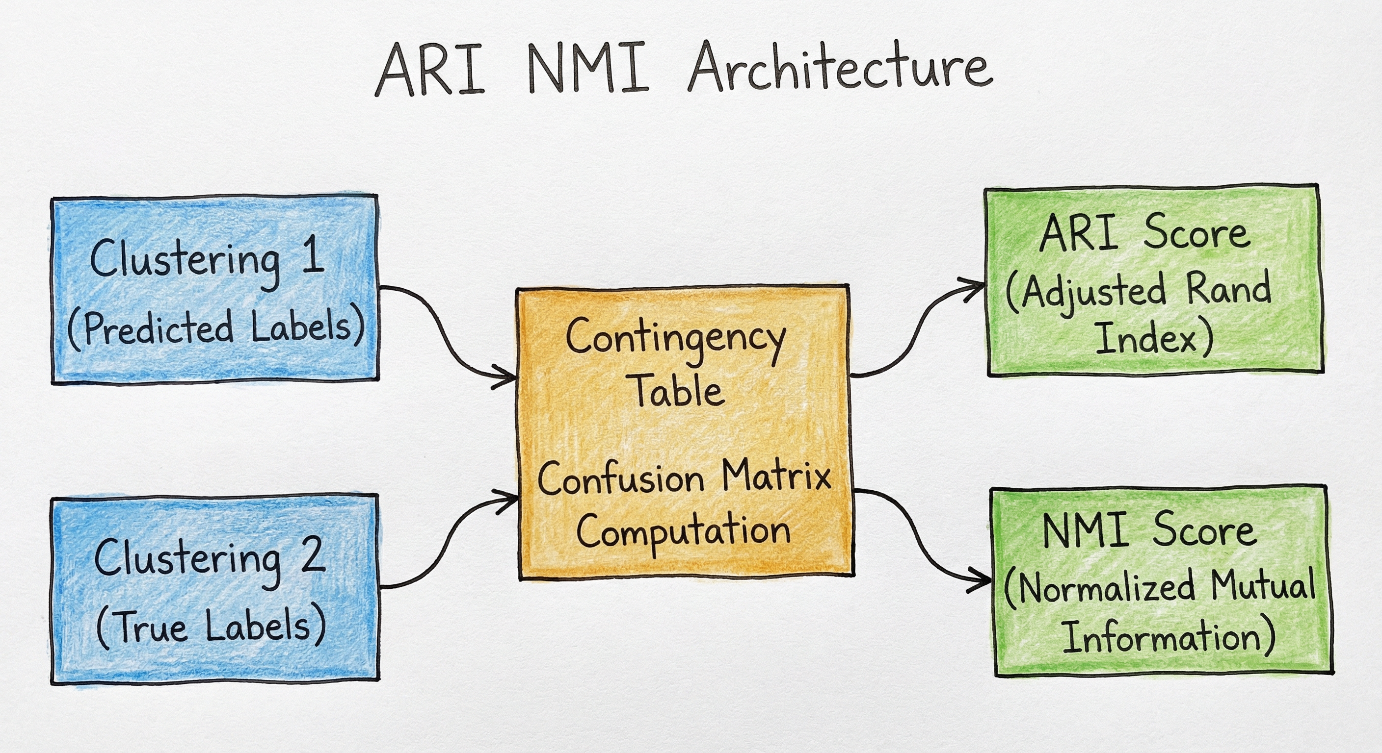
A directed flow where predicted labels and true labels both feed into a contingency table builder. The contingency table feeds into two parallel paths: one computing pair counts leading to the ARI score, and another computing entropy and mutual information leading to the NMI score and its V-measure decomposition into homogeneity and completeness.
How to Implement
Computing ARI and NMI in Practice
The good news: implementing ARI and NMI from scratch is straightforward, and battle-tested implementations exist in every major ML library. The computation is dominated by contingency table construction ( with hash maps or with direct indexing), followed by arithmetic operations on the table.
For production systems, always use scikit-learn's adjusted_rand_score() and normalized_mutual_info_score(). They handle edge cases correctly (empty clusters, single-element clusters, identical partitions) and use optimized sparse matrix operations for large numbers of clusters.
NMI Normalization Choices
A common source of confusion is scikit-learn's average_method parameter for NMI. Before version 0.22, the default was 'geometric' (Strehl-Ghosh formulation). Since 0.22, the default is 'arithmetic', which equals V-measure. This means old code and new code compute slightly different NMI values. Always specify the normalization explicitly for reproducibility.
When to Use AMI Instead of NMI
If your clustering produces many small clusters (e.g., DBSCAN with a tight epsilon), NMI can be inflated because many clusters = high entropy = high mutual information even by chance. The Adjusted Mutual Information (AMI) corrects for this, analogous to how ARI corrects the Rand Index. Use AMI when comparing algorithms that produce very different numbers of clusters.
Cost Note: For a customer segmentation pipeline at a fintech startup in Bengaluru processing 5M customer records with 20 clusters, computing ARI + NMI takes under 500ms on a single CPU core. Even bootstrapping 1000 resamples for confidence intervals completes in under 10 minutes. The cost of evaluation compute (~₹5 or $0.06 on AWS t3.medium) is negligible compared to the cost of deploying a bad clustering.
from sklearn.metrics import (
    adjusted_rand_score,
    normalized_mutual_info_score,
    adjusted_mutual_info_score,
    v_measure_score,
    homogeneity_score,
    completeness_score,
)
import numpy as np

# Ground truth labels and predicted cluster assignments
labels_true = np.array([0, 0, 0, 1, 1, 1, 2, 2, 2])
labels_pred = np.array([0, 0, 1, 1, 1, 1, 2, 2, 2])

# Adjusted Rand Index
ari = adjusted_rand_score(labels_true, labels_pred)
print(f"ARI: {ari:.4f}")  # 0.5714

# Normalized Mutual Information (arithmetic mean normalization)
nmi = normalized_mutual_info_score(labels_true, labels_pred, average_method='arithmetic')
print(f"NMI (arithmetic): {nmi:.4f}")

# NMI with geometric mean (legacy default)
nmi_geom = normalized_mutual_info_score(labels_true, labels_pred, average_method='geometric')
print(f"NMI (geometric): {nmi_geom:.4f}")

# Adjusted Mutual Information (chance-corrected)
ami = adjusted_mutual_info_score(labels_true, labels_pred)
print(f"AMI: {ami:.4f}")

# V-measure decomposition
homogeneity = homogeneity_score(labels_true, labels_pred)
completeness = completeness_score(labels_true, labels_pred)
v_measure = v_measure_score(labels_true, labels_pred)
print(f"Homogeneity: {homogeneity:.4f}")
print(f"Completeness: {completeness:.4f}")
print(f"V-measure: {v_measure:.4f}")
This shows the full family of external clustering metrics available in scikit-learn. Notice how labels_true and labels_pred are simple integer arrays -- no probabilities needed, unlike classification metrics like ROC-AUC. The average_method parameter for NMI is crucial for reproducibility: always specify it explicitly. V-measure decomposes NMI into homogeneity (are clusters pure?) and completeness (are classes in one cluster?), which gives you more diagnostic information than a single score.
from sklearn.cluster import KMeans, DBSCAN, AgglomerativeClustering
from sklearn.datasets import make_blobs
from sklearn.metrics import adjusted_rand_score, normalized_mutual_info_score
from sklearn.preprocessing import StandardScaler
import numpy as np

# Generate synthetic data with known ground truth
X, y_true = make_blobs(
    n_samples=1000, centers=5, cluster_std=1.2, random_state=42
)
X = StandardScaler().fit_transform(X)

# Define clustering algorithms to compare
algorithms = {
    'KMeans (k=5)': KMeans(n_clusters=5, random_state=42, n_init=10),
    'KMeans (k=3)': KMeans(n_clusters=3, random_state=42, n_init=10),
    'KMeans (k=10)': KMeans(n_clusters=10, random_state=42, n_init=10),
    'DBSCAN (eps=0.5)': DBSCAN(eps=0.5, min_samples=5),
    'Agglomerative (k=5)': AgglomerativeClustering(n_clusters=5),
}

print(f"{'Algorithm':<25} {'ARI':>8} {'NMI':>8} {'Clusters':>10}")
print('-' * 55)

for name, algo in algorithms.items():
    labels_pred = algo.fit_predict(X)
    n_clusters = len(set(labels_pred)) - (1 if -1 in labels_pred else 0)
    ari = adjusted_rand_score(y_true, labels_pred)
    nmi = normalized_mutual_info_score(y_true, labels_pred, average_method='arithmetic')
    print(f"{name:<25} {ari:>8.4f} {nmi:>8.4f} {n_clusters:>10}")
This is the typical workflow: compare several clustering algorithms on the same data using both ARI and NMI. Notice how K-means with the wrong k (3 or 10) will show lower scores than k=5 (the true number of clusters). DBSCAN may find a different number of clusters and assign some points as noise (-1 label). When DBSCAN produces noise points, they form their own implicit group in the contingency table. This pattern is useful for hyperparameter tuning -- you can sweep k values and pick the one with the highest ARI/NMI.
import numpy as np
from scipy.special import comb
from sklearn.metrics.cluster import contingency_matrix

def ari_from_scratch(labels_true, labels_pred):
    """Compute ARI using the contingency table approach."""
    # Build contingency table
    contingency = contingency_matrix(labels_true, labels_pred)

    # Sum of C(n_ij, 2) over all cells
    sum_comb_nij = sum(
        comb(n_ij, 2) for n_ij in contingency.flatten()
    )

    # Row sums and column sums
    row_sums = contingency.sum(axis=1)
    col_sums = contingency.sum(axis=0)

    # Sum of C(a_i, 2) and C(b_j, 2)
    sum_comb_rows = sum(comb(a, 2) for a in row_sums)
    sum_comb_cols = sum(comb(b, 2) for b in col_sums)

    # Total number of pairs
    n = contingency.sum()
    total_pairs = comb(n, 2)

    # Expected index under random model
    expected = (sum_comb_rows * sum_comb_cols) / total_pairs

    # Maximum index
    max_index = 0.5 * (sum_comb_rows + sum_comb_cols)

    # ARI formula
    numerator = sum_comb_nij - expected
    denominator = max_index - expected

    if denominator == 0:
        return 1.0  # Both partitions are identical singletons

    return numerator / denominator

def nmi_from_scratch(labels_true, labels_pred, average_method='arithmetic'):
    """Compute NMI using contingency table."""
    contingency = contingency_matrix(labels_true, labels_pred)
    n = contingency.sum()

    # Marginal distributions
    p_i = contingency.sum(axis=1) / n  # P(U)
    p_j = contingency.sum(axis=0) / n  # P(V)

    # Entropies
    H_U = -np.sum(p_i[p_i > 0] * np.log(p_i[p_i > 0]))
    H_V = -np.sum(p_j[p_j > 0] * np.log(p_j[p_j > 0]))

    # Mutual information
    MI = 0.0
    for i in range(contingency.shape[0]):
        for j in range(contingency.shape[1]):
            if contingency[i, j] > 0:
                p_ij = contingency[i, j] / n
                MI += p_ij * np.log(p_ij / (p_i[i] * p_j[j]))

    # Normalize
    if average_method == 'arithmetic':
        normalizer = (H_U + H_V) / 2
    elif average_method == 'geometric':
        normalizer = np.sqrt(H_U * H_V)
    elif average_method == 'min':
        normalizer = min(H_U, H_V)
    elif average_method == 'max':
        normalizer = max(H_U, H_V)
    else:
        raise ValueError(f"Unknown average_method: {average_method}")

    if normalizer == 0:
        return 1.0  # Both partitions have zero entropy (all same label)

    return MI / normalizer

# Test
labels_true = np.array([0, 0, 0, 1, 1, 1, 2, 2, 2])
labels_pred = np.array([0, 0, 1, 1, 1, 1, 2, 2, 2])

print(f"ARI (from scratch): {ari_from_scratch(labels_true, labels_pred):.4f}")
print(f"NMI (from scratch): {nmi_from_scratch(labels_true, labels_pred):.4f}")
This from-scratch implementation reveals the internals of both metrics. For ARI, the key is computing binomial coefficients from the contingency table entries and marginal sums, then applying the chance-correction formula. For NMI, you compute entropies from marginal distributions and mutual information from the joint distribution. Note the edge cases: zero entries in the contingency table contribute 0 to MI (by the convention that ), and when both partitions have zero entropy (all points in one cluster), we return 1.0. In production, always use scikit-learn's optimized implementation, but understanding the internals helps you debug unexpected results.
from sklearn.metrics import adjusted_rand_score, normalized_mutual_info_score
import numpy as np

def bootstrap_clustering_metrics(
    labels_true, labels_pred, n_bootstraps=2000, confidence=0.95, seed=42
):
    """Compute bootstrap confidence intervals for ARI and NMI."""
    rng = np.random.RandomState(seed)
    n = len(labels_true)

    ari_scores = []
    nmi_scores = []

    for _ in range(n_bootstraps):
        # Resample with replacement
        indices = rng.randint(0, n, size=n)
        lt = labels_true[indices]
        lp = labels_pred[indices]

        # Skip degenerate samples (all one label)
        if len(np.unique(lt)) < 2 or len(np.unique(lp)) < 2:
            continue

        ari_scores.append(adjusted_rand_score(lt, lp))
        nmi_scores.append(normalized_mutual_info_score(
            lt, lp, average_method='arithmetic'
        ))

    alpha = (1 - confidence) / 2
    results = {
        'ari': {
            'point': adjusted_rand_score(labels_true, labels_pred),
            'ci_lower': np.percentile(ari_scores, 100 * alpha),
            'ci_upper': np.percentile(ari_scores, 100 * (1 - alpha)),
        },
        'nmi': {
            'point': normalized_mutual_info_score(
                labels_true, labels_pred, average_method='arithmetic'
            ),
            'ci_lower': np.percentile(nmi_scores, 100 * alpha),
            'ci_upper': np.percentile(nmi_scores, 100 * (1 - alpha)),
        }
    }
    return results

# Example usage
np.random.seed(42)
labels_true = np.repeat([0, 1, 2, 3, 4], 200)  # 1000 points, 5 classes
labels_pred = labels_true.copy()
# Introduce some noise: randomly flip 10% of labels
flip_mask = np.random.random(1000) < 0.10
labels_pred[flip_mask] = np.random.randint(0, 5, size=flip_mask.sum())

results = bootstrap_clustering_metrics(labels_true, labels_pred)

for metric, vals in results.items():
    print(
        f"{metric.upper()}: {vals['point']:.4f} "
        f"(95% CI: [{vals['ci_lower']:.4f}, {vals['ci_upper']:.4f}])"
    )
Bootstrap confidence intervals are essential for claiming statistical significance when comparing clustering algorithms. This implementation resamples data points with replacement, recomputes ARI and NMI on each bootstrap sample, and extracts percentile-based confidence intervals. Note the degenerate sample check: if a bootstrap sample happens to contain only one unique true or predicted label, both metrics are undefined, so we skip it. With 2000 resamples, you get stable 95% CI estimates. Report these in papers and model cards -- a point estimate without uncertainty is incomplete.
from sklearn.cluster import KMeans
from sklearn.datasets import make_blobs
from sklearn.metrics import (
    adjusted_rand_score,
    normalized_mutual_info_score,
    silhouette_score,
)
from sklearn.preprocessing import StandardScaler
import numpy as np
import matplotlib.pyplot as plt

# Generate data with 5 true clusters
X, y_true = make_blobs(n_samples=2000, centers=5, cluster_std=1.5, random_state=42)
X = StandardScaler().fit_transform(X)

# Sweep k from 2 to 15
k_range = range(2, 16)
ari_scores = []
nmi_scores = []
sil_scores = []

for k in k_range:
    kmeans = KMeans(n_clusters=k, random_state=42, n_init=10)
    labels_pred = kmeans.fit_predict(X)

    ari_scores.append(adjusted_rand_score(y_true, labels_pred))
    nmi_scores.append(normalized_mutual_info_score(
        y_true, labels_pred, average_method='arithmetic'
    ))
    sil_scores.append(silhouette_score(X, labels_pred))

# Plot
fig, axes = plt.subplots(1, 3, figsize=(15, 4))

axes[0].plot(k_range, ari_scores, 'bo-', linewidth=2)
axes[0].axvline(x=5, color='red', linestyle='--', label='True k=5')
axes[0].set_xlabel('Number of clusters (k)')
axes[0].set_ylabel('ARI')
axes[0].set_title('Adjusted Rand Index vs k')
axes[0].legend()
axes[0].grid(alpha=0.3)

axes[1].plot(k_range, nmi_scores, 'go-', linewidth=2)
axes[1].axvline(x=5, color='red', linestyle='--', label='True k=5')
axes[1].set_xlabel('Number of clusters (k)')
axes[1].set_ylabel('NMI')
axes[1].set_title('NMI vs k')
axes[1].legend()
axes[1].grid(alpha=0.3)

axes[2].plot(k_range, sil_scores, 'rs-', linewidth=2)
axes[2].axvline(x=5, color='red', linestyle='--', label='True k=5')
axes[2].set_xlabel('Number of clusters (k)')
axes[2].set_ylabel('Silhouette Score')
axes[2].set_title('Silhouette vs k')
axes[2].legend()
axes[2].grid(alpha=0.3)

plt.tight_layout()
plt.savefig('clustering_metrics_vs_k.png', dpi=150)
plt.show()

# Best k according to each metric
print(f"Best k (ARI): {k_range[np.argmax(ari_scores)]}")
print(f"Best k (NMI): {k_range[np.argmax(nmi_scores)]}")
print(f"Best k (Silhouette): {k_range[np.argmax(sil_scores)]}")
This demonstrates a common pattern: using ARI and NMI to select the optimal number of clusters when ground truth is available (e.g., during development with labeled data). Both ARI and NMI peak at the true k=5. Silhouette score (an internal metric that doesn't need ground truth) is shown for comparison. The key insight: external metrics like ARI/NMI are strictly better than internal metrics when ground truth exists, but internal metrics are your only option in production when labels aren't available. This pattern is especially useful for validating that your chosen algorithm and hyperparameters recover known structure before deploying to unlabeled production data.
# Scikit-learn clustering evaluation configuration

from sklearn.metrics import (
    adjusted_rand_score,
    normalized_mutual_info_score,
    adjusted_mutual_info_score,
    v_measure_score,
    homogeneity_score,
    completeness_score,
    fowlkes_mallows_score,
)

# Standard ARI (no parameters needed)
ari = adjusted_rand_score(labels_true, labels_pred)

# NMI with explicit normalization
nmi_arith = normalized_mutual_info_score(labels_true, labels_pred, average_method='arithmetic')
nmi_geom = normalized_mutual_info_score(labels_true, labels_pred, average_method='geometric')
nmi_min = normalized_mutual_info_score(labels_true, labels_pred, average_method='min')
nmi_max = normalized_mutual_info_score(labels_true, labels_pred, average_method='max')

# Chance-corrected mutual information
ami = adjusted_mutual_info_score(labels_true, labels_pred, average_method='arithmetic')

# Full V-measure decomposition
homogeneity, completeness, v_measure = (
    homogeneity_score(labels_true, labels_pred),
    completeness_score(labels_true, labels_pred),
    v_measure_score(labels_true, labels_pred),
)

# Fowlkes-Mallows (geometric mean of precision and recall for pairs)
fmi = fowlkes_mallows_score(labels_true, labels_pred)
Common Implementation Mistakes
- ●
Confusing NMI normalization variants: scikit-learn changed the default
average_methodfrom'geometric'to'arithmetic'in version 0.22. If you're comparing NMI values from papers or older codebases, make sure the normalization matches. Always explicitly specifyaverage_method='arithmetic'(or whichever you prefer) for reproducibility. - ●
Using NMI when you should use AMI: NMI is not adjusted for chance. When comparing clusterings with very different numbers of clusters (e.g., k=2 vs k=50), NMI will favor the finer-grained clustering even if it's random. Use
adjusted_mutual_info_score()when the number of clusters varies widely. - ●
Treating ARI as a percentage: ARI = 0.6 does not mean "60% correct." It means agreement is 60% of the way from chance-level to perfect, after correcting for expected random agreement. This is a common misinterpretation in presentations and reports.
- ●
Ignoring the sign of ARI: Negative ARI means your clustering is worse than random -- the algorithm is actively putting similar points in different clusters. This can happen with poor initialization, wrong distance metric, or inappropriate k. A negative ARI should trigger investigation, not just disappointment.
- ●
Applying external metrics without ground truth: ARI and NMI require true labels. If you only have cluster assignments (no ground truth), use internal metrics like Silhouette Score or Davies-Bouldin Index. This sounds obvious, but practitioners sometimes fabricate "pseudo-ground-truth" from heuristics, which defeats the purpose.
- ●
Not permutation-checking labels: Both ARI and NMI are permutation-invariant, so cluster labels don't need to match ground truth labels numerically. If true class 0 maps to predicted cluster 3, that's fine -- the metrics handle it. Don't waste time trying to align label indices.
When Should You Use This?
Use When
You have ground truth labels and want to evaluate how well a clustering algorithm recovers the known structure -- the core use case for external validation
You're comparing multiple clustering algorithms (K-means, DBSCAN, hierarchical, spectral) on the same dataset and need a fair, standardized metric
You're tuning hyperparameters like the number of clusters k and want to identify the value that best matches known categories
You need a permutation-invariant metric that doesn't require matching cluster label indices to ground truth label indices
You want complementary perspectives -- ARI for pairwise agreement and NMI for information content -- to get a robust evaluation
You're running clustering benchmarks and need metrics that are standard in the academic literature, making your results comparable to published work
Your clustering is part of a larger pipeline (e.g., topic modeling, customer segmentation) and you need to validate it during development using labeled validation data
Avoid When
You don't have ground truth labels -- use internal metrics (Silhouette Score, Davies-Bouldin Index, Calinski-Harabasz Index) instead
Your ground truth has significantly more or fewer categories than your clustering, and you haven't considered the implications for metric behavior (NMI can inflate with many clusters; ARI can underpenalize merging)
You're evaluating soft/fuzzy clustering where points have partial memberships in multiple clusters -- standard ARI and NMI require hard assignments
You care about specific cluster properties (compactness, separation, density) rather than agreement with ground truth -- internal metrics are more appropriate
Your application requires real-time evaluation during streaming data ingestion -- while ARI/NMI are fast (), they require the full ground truth to be available, which is rarely the case in streaming
You're comparing clusterings of different datasets or different subsets of the same dataset -- ARI and NMI are only meaningful when comparing partitions of the same set of objects
Key Tradeoffs
ARI vs NMI: When Do They Disagree?
The most important tradeoff is between ARI and NMI themselves. They measure different things and can diverge:
| Scenario | ARI Behavior | NMI Behavior |
|---|---|---|
| Predicted k matches true k, good assignment | High | High |
| Predicted k >> true k (over-splitting) | Drops moderately | Can stay high (pure micro-clusters) |
| Predicted k << true k (under-splitting) | Drops | Drops |
| Random clustering | ~0 | Can be > 0 (not chance-corrected) |
| Worse than random | Negative | Always >= 0 |
Key takeaway: NMI can be misleadingly high when the clustering is over-split (many pure but tiny clusters). ARI is more conservative and penalizes over-splitting. If NMI is high but ARI is moderate, your algorithm is likely finding pure sub-clusters within each class. If you want to catch this, use AMI instead of NMI.
Chance Correction: ARI and AMI vs NMI
ARI is corrected for chance by definition. NMI is not. This matters when the number of clusters is large relative to the number of data points. For example, with data points and clusters, a random clustering will have NMI significantly above 0 just by chance. AMI (Adjusted Mutual Information) fixes this.
Practical guideline: If all algorithms produce similar numbers of clusters, NMI is fine. If some algorithms produce 5 clusters and others produce 50, use AMI to avoid biasing the comparison.
Sensitivity to Partition Structure
ARI is based on pair counting, so it's most sensitive to the exact assignment of data points. NMI is based on information content, so it's more sensitive to the overall distributional agreement between cluster and class membership. For imbalanced ground truth (one class has 80% of points), ARI tends to be dominated by the large class, while NMI gives more balanced weight to minority classes through the logarithmic terms.
Rule of Thumb: Report both ARI and NMI. If they agree, you have a robust evaluation. If they diverge, investigate the cluster structure (over-splitting, under-splitting, class imbalance) to understand why.
Alternatives & Comparisons
Silhouette Score is an internal metric that doesn't require ground truth labels -- it measures cluster cohesion vs separation using only the data and predicted labels. Choose Silhouette when you have no ground truth. Choose ARI/NMI when you do have ground truth, as they directly measure agreement with known structure, which is a stronger form of validation. Silhouette can also be high for poor clusterings if clusters happen to be compact but don't match the real categories.
Davies-Bouldin is another internal metric (lower is better) that measures the ratio of within-cluster scatter to between-cluster separation. Like Silhouette, it needs no ground truth. Choose ARI/NMI when ground truth is available for a direct, authoritative validation. Davies-Bouldin is useful for selecting k during deployment when labels aren't available, but it can favor spherical clusters and penalize non-convex shapes that DBSCAN handles well.
Calinski-Harabasz (Variance Ratio Criterion) is an internal metric (higher is better) based on the ratio of between-cluster dispersion to within-cluster dispersion. It's fast and conceptually simple but assumes clusters are convex and isotropic. ARI/NMI make no assumptions about cluster shape -- they only care about label agreement. Use Calinski-Harabasz for fast internal validation during development; use ARI/NMI for definitive external validation when ground truth exists.
FMI is the geometric mean of pairwise precision and recall, providing a pair-counting metric similar to ARI. Unlike ARI, FMI is not corrected for chance, so random clusterings can score above zero. Unlike NMI, it's not information-theoretic. ARI is generally preferred over FMI because chance correction is important when comparing clusterings with different numbers of clusters. FMI is mainly useful when you want a pair-counting metric on the [0, 1] scale without chance correction.
You can compute a confusion matrix between true labels and predicted clusters after solving the optimal label assignment problem (Hungarian algorithm). This gives you per-class precision/recall, which ARI and NMI don't provide. Choose the confusion matrix approach when you need per-class diagnostic detail. Choose ARI/NMI when you need a single summary score for comparison, especially when the number of clusters differs from the number of true classes.
Pros, Cons & Tradeoffs
Advantages
Chance correction in ARI ensures that random clusterings score near 0, providing a meaningful baseline. Without this, a metric like raw Rand Index gives misleadingly high scores for random partitions, especially with many clusters.
Permutation invariance means cluster label indices don't need to match ground truth indices. Cluster 0 can correspond to class 3, and the metrics handle it automatically -- no Hungarian matching needed.
Complementary perspectives: ARI (pair-counting) and NMI (information-theoretic) capture different facets of clustering quality. Reporting both gives a robust, multi-faceted evaluation that's hard to game.
Computationally efficient at time and space. For typical clustering problems with M and , both metrics compute in milliseconds -- negligible compared to the clustering algorithm itself.
Well-established theoretical properties: both metrics have been studied extensively since the 1980s-2000s. Their behavior under various conditions (imbalanced classes, different k values, noise) is well-understood, making interpretation reliable.
Symmetric: and . You can compare two clusterings without designating one as "ground truth" -- useful for consensus clustering and ensemble evaluation.
Standard in academic literature: virtually every clustering paper reports ARI and/or NMI, making your results directly comparable to published benchmarks across computer science, bioinformatics, and social science.
Disadvantages
Requires ground truth labels, which are rarely available in real-world clustering scenarios. This limits ARI/NMI to development-time validation, benchmarking, and semi-supervised settings -- you can't use them for production monitoring without labeled data.
NMI is not adjusted for chance: it can be inflated when comparing clusterings with many clusters relative to the data size. Practitioners often don't realize this and report overoptimistic NMI values. AMI exists but is less commonly used.
ARI can be dominated by large clusters in imbalanced settings. If one true class has 90% of the data, getting that class right dominates the pairwise comparison, potentially masking poor performance on minority classes.
No diagnostic detail: both metrics produce a single scalar. They don't tell you which clusters or classes are problematic. You need supplementary analysis (confusion matrix, per-class homogeneity) to understand failure patterns.
Sensitive to noise labeling conventions: DBSCAN assigns noise points label -1. How these are handled (as a separate cluster or excluded) affects ARI/NMI values. scikit-learn treats -1 as a valid cluster label, which may not match your intent.
Hard assignment only: standard ARI and NMI require each point to belong to exactly one cluster. For soft/fuzzy clustering (e.g., Gaussian Mixture Models with soft assignments), you must discretize memberships first, losing information.
Failure Modes & Debugging
NMI Inflation with Over-Splitting
Cause
The clustering algorithm produces many more clusters than the true number of classes (e.g., DBSCAN with tight epsilon or K-means with k=50 when the true number is 5). Each predicted cluster is very pure (contains only one class), leading to high homogeneity and high NMI -- but the clustering is not useful because each true class is split into many fragments.
Symptoms
NMI is surprisingly high (0.85+) while ARI is moderate (0.5-0.6). Completeness score is low even though homogeneity is high. The number of predicted clusters far exceeds the true number of classes. Downstream applications that depend on grouping (e.g., batch marketing emails per cluster) fail because groups are too fragmented.
Mitigation
Always report ARI alongside NMI to catch this divergence. Use Adjusted Mutual Information (AMI) instead of NMI when comparing algorithms that produce different numbers of clusters. Check the homogeneity-completeness decomposition: if homogeneity >> completeness, over-splitting is the problem. Consider using min normalization for NMI, which equals completeness and penalizes splitting.
Chance Agreement Masquerading as Clustering Quality
Cause
Using raw Rand Index or unnormalized Mutual Information instead of their adjusted versions. With many clusters and data points, random agreement between two partitions can be substantial, especially when cluster sizes happen to be similar.
Symptoms
Raw RI scores 0.7-0.9 even on random clusterings. NMI reports 0.15-0.30 for clearly random partitions. Team celebrates "decent" clustering performance that is actually no better than chance. This is especially dangerous with small datasets (n < 200) and many clusters (k > 10).
Mitigation
Always use ARI (not RI) and consider AMI (not NMI) for pair-counting and information-theoretic evaluation respectively. Establish a baseline by computing ARI/NMI on random permutations of the labels. If your algorithm's score is not significantly above this baseline (e.g., using bootstrap confidence intervals), the clustering has not found meaningful structure.
Imbalanced Ground Truth Biasing ARI
Cause
One or two true classes dominate the dataset (e.g., 80% of customers in one segment). ARI's pairwise calculation is dominated by pairs from the majority class. Getting the majority class right produces a high ARI even if minority classes are completely wrong.
Symptoms
ARI is 0.75+ but per-class analysis reveals that small classes (5-10% of data) are misassigned to the dominant cluster. Marketing team targets the wrong customers in minority segments. NMI may be lower than ARI because its logarithmic terms give more weight to minority classes.
Mitigation
Supplement ARI with per-class metrics: compute homogeneity and completeness scores, inspect the confusion matrix between true and predicted labels (with Hungarian matching), and calculate per-class recall. Consider weighting ARI by class size inversely or using NMI which handles imbalance more gracefully through entropy-based weighting.
DBSCAN Noise Label Distortion
Cause
DBSCAN assigns noise points the label -1. scikit-learn's adjusted_rand_score and normalized_mutual_info_score treat -1 as a valid cluster label, grouping all noise points into one "noise cluster." If many points are labeled as noise, this artificial cluster distorts the contingency table.
Symptoms
ARI/NMI scores are unexpectedly low even when DBSCAN correctly identifies the core clusters. The noise "cluster" contains points from many true classes, creating a row in the contingency table with high entropy. Reducing DBSCAN's min_samples or eps to capture more points as non-noise dramatically changes ARI/NMI.
Mitigation
Filter out noise points (label == -1) before computing ARI/NMI: mask = labels_pred != -1; ari = adjusted_rand_score(labels_true[mask], labels_pred[mask]). Alternatively, report the fraction of noise points alongside ARI/NMI so that readers understand the coverage-quality tradeoff. Some practitioners assign noise points to the nearest cluster centroid before evaluation.
Small Sample Instability
Cause
With small datasets (), the contingency table has few entries, making both ARI and NMI highly sensitive to individual point assignments. Moving a single point between clusters can swing ARI by 0.1 or more.
Symptoms
ARI/NMI values are volatile across cross-validation folds or bootstrap resamples. Confidence intervals are very wide (e.g., ARI = 0.65 with 95% CI [0.35, 0.90]). Minor changes to preprocessing (e.g., feature scaling) cause large metric swings.
Mitigation
Always report bootstrap confidence intervals for ARI/NMI. Use stratified resampling to ensure all classes appear in each fold. For very small datasets, consider exact permutation tests instead of asymptotic approximations. Collect more labeled data if possible -- evaluation metrics are only as reliable as the data they're computed on.
Mismatched Granularity Between Prediction and Ground Truth
Cause
The predicted clustering operates at a different granularity than the ground truth. For example, ground truth has 3 broad categories ("small business", "enterprise", "government") but the clustering finds 15 fine-grained sub-segments. Or vice versa: ground truth has 20 fine categories but the algorithm merges them into 3 clusters.
Symptoms
Both ARI and NMI are moderate (0.4-0.6) despite the clustering being useful at its own granularity. Stakeholders dismiss the clustering as "poor" based on metrics alone, even though the sub-clusters reveal actionable structure within each broad category.
Mitigation
Consider hierarchical evaluation: assess the clustering at multiple granularity levels using dendrogram cutting. Use the V-measure decomposition to distinguish between homogeneity issues (impure clusters) and completeness issues (split classes). Discuss with domain experts whether the ground truth granularity matches the business need -- sometimes the clustering reveals a better categorization than the original labels.
Placement in an ML System
Where ARI/NMI Fit in the ML Pipeline
ARI and NMI live in the evaluation phase of a clustering pipeline, after the clustering algorithm has produced assignments and before the deployment decision.
During Development: When you have labeled validation data (e.g., manually annotated customer segments, known cell types in a scRNA-seq experiment, or benchmark datasets like MNIST), use ARI and NMI to evaluate and compare clustering algorithms. Sweep hyperparameters (k for K-means, epsilon/min_samples for DBSCAN) and select the configuration that maximizes ARI/NMI.
Validating Internal Metrics: In production, you won't have ground truth labels, so you'll rely on internal metrics (Silhouette Score, Davies-Bouldin Index). But during development, compute both internal and external metrics. If Silhouette and ARI agree on the best algorithm, you can trust Silhouette to guide production monitoring. If they disagree, investigate why -- Silhouette rewards compact clusters, which may not match the true class structure.
Benchmark Reporting: In academic papers and internal reports, ARI and NMI are the standard metrics for clustering evaluation. They make your results comparable to published work and provide a shared language for discussing clustering quality across teams.
Consensus Clustering: When combining multiple clusterings (ensemble methods), ARI can measure agreement between individual clusterings to weight them in the consensus. Since ARI is symmetric, you can build a similarity matrix between all pairs of clusterings and use it for meta-clustering.
Key Insight: ARI and NMI are development-time metrics. Once you deploy a clustering system without ground truth, you switch to internal metrics for monitoring. But the ARI/NMI evaluation during development is what gives you confidence that your internal metrics are tracking the right thing.
Pipeline Stage
Evaluation / Validation
Upstream
- Clustering Algorithm (K-means, DBSCAN, hierarchical, spectral)
- Feature Engineering / Embedding Generation
- Dimensionality Reduction (PCA, t-SNE, UMAP)
Downstream
- Model Selection (choosing best clustering algorithm/hyperparameters)
- Hyperparameter Tuning (optimal k, epsilon, min_samples)
- Deployment Decision (is clustering good enough for production?)
- Internal Metric Validation (correlating Silhouette with ARI/NMI)
Scaling Bottlenecks
For a single evaluation on data points with and clusters, ARI and NMI are both -- essentially linear in data size. This is negligible for most applications:
- K, : ~10ms on a single core
- M, : ~2 seconds (dominated by contingency table construction)
Bottlenecks appear in three scenarios:
1. Many-cluster DBSCAN: If DBSCAN produces micro-clusters, the contingency table becomes large. For , the table has 100M entries. Use sparse contingency matrices (scikit-learn does this automatically) to reduce memory from to .
2. Bootstrapping with Large n: 2000 bootstrap resamples on M takes 30 minutes on one core. Parallelize across cores using ₹2,500/$30 per hour on AWS c5.4xlarge), this drops to ~2 minutes.joblib or multiprocessing. On a 16-core machine (
3. Hyperparameter Grid Search: Evaluating 50 k-values with 5-fold CV = 250 evaluations. For K per fold, total evaluation time is 250 * 10ms = 2.5 seconds -- still fast, but the clustering itself is the bottleneck.
Production Case Studies
E-commerce companies like Flipkart and Amazon India use clustering to segment customers into behavioral groups (price-sensitive, brand-loyal, impulse buyers, etc.) for targeted marketing campaigns. During development, the data science team validates clustering quality against manually labeled customer segments from marketing domain experts. A multi-metric evaluation framework combining ARI, NMI, homogeneity, completeness, and V-measure alongside internal metrics (Silhouette, DBI) provides a comparative assessment of K-Means vs. Hierarchical Clustering for operational guidance. The external metrics ensure that data-driven segments align with business-defined personas, not just statistical structure.
Using ARI and NMI to validate against expert-labeled segments improved marketing campaign targeting accuracy by identifying that K-Means with k=7 best matched the known customer personas (ARI = 0.72, NMI = 0.78). Hierarchical clustering produced more granular segments (k=12) with higher NMI (0.83) but lower ARI (0.58), indicating over-splitting. The team chose K-Means for campaign targeting and used hierarchical sub-segments for personalization within each broad persona.
Single-cell RNA sequencing (scRNA-seq) generates gene expression profiles for thousands of individual cells. Clustering these profiles reveals cell types -- a fundamental task in modern genomics. Research groups at IISC Bangalore and IIT Delhi use ARI and NMI to evaluate whether clustering algorithms (Louvain, Leiden, K-means on PCA embeddings) correctly recover known cell type labels. A rapid review of clustering algorithms across 20+ benchmark scRNA-seq datasets showed that ARI and NMI are the two most commonly reported metrics, with modern graph-based algorithms (Leiden) achieving ARI > 0.85 on well-separated cell types.
Benchmarking across 8 scRNA-seq datasets with known cell type annotations, the Leiden algorithm consistently achieved ARI = 0.82-0.91 and NMI = 0.85-0.93, outperforming K-means (ARI = 0.65-0.78) and hierarchical clustering (ARI = 0.60-0.75). The ARI-NMI divergence on heterogeneous datasets (ARI = 0.72, NMI = 0.88) helped identify over-splitting of rare cell populations, leading researchers to merge sub-clusters before downstream differential expression analysis.
Social network analysis relies on community detection algorithms (Louvain, Infomap, Label Propagation) to find groups of densely connected users. Vinh, Epps, and Bailey's comprehensive study on information-theoretic measures demonstrated that NMI is the dominant metric for evaluating community detection in networks like Facebook, Twitter, and Indian social platforms. They analyzed how different normalization strategies affect NMI values and showed that chance correction (AMI) is essential when comparing algorithms that produce very different numbers of communities. The Lancichinetti-Fortunato-Radicchi (LFR) benchmark provides synthetic networks with planted community structure, enabling ARI/NMI evaluation.
The study demonstrated that NMI without chance correction overestimated the quality of algorithms producing many small communities (NMI = 0.75 vs AMI = 0.45 for the same partition). On LFR benchmark networks with 1000-10000 nodes, Infomap achieved the highest ARI (0.88-0.95) and NMI (0.90-0.97) for well-separated communities, while all algorithms degraded gracefully as community mixing increased. The paper established best practices for reporting NMI variants that are now standard in the community detection literature.
NLP teams at Indian tech companies and research labs use document clustering to organize large text corpora into topics. The 20 Newsgroups dataset is a classic benchmark where 20 known topic categories serve as ground truth. scikit-learn's clustering evaluation tutorial demonstrates how ARI and NMI evaluate K-means and spectral clustering on TF-IDF representations of these documents. The tutorial also shows the critical importance of chance adjustment: raw Rand Index and unnormalized MI both inflate scores for random clusterings, while ARI and AMI correctly score them near zero.
On the 20 Newsgroups dataset (~18K documents, 20 classes), K-means on TF-IDF features achieved ARI = 0.35 and NMI = 0.48, reflecting the inherent difficulty of overlapping topic categories. Spectral clustering improved to ARI = 0.42 and NMI = 0.55. The chance correction demonstration showed that random labelings scored RI = 0.89 but ARI = -0.001, dramatically illustrating why adjusted metrics are essential. These benchmarks are widely cited by Indian graduate students and practitioners as a reference for expected metric ranges.
Tooling & Ecosystem
The gold standard for clustering evaluation in Python. Provides adjusted_rand_score(), normalized_mutual_info_score(), adjusted_mutual_info_score(), v_measure_score(), homogeneity_score(), completeness_score(), and fowlkes_mallows_score(). All operate on label arrays and handle edge cases (empty clusters, single-class partitions). Uses sparse contingency matrices for memory efficiency with many clusters. Extensive documentation with visual examples.
GPU-accelerated clustering metrics for PyTorch workflows. Provides AdjustedRandScore and NormalizedMutualInfoScore as TorchMetrics classes that integrate with PyTorch Lightning training loops. Useful when clustering is part of a deep learning pipeline (e.g., deep clustering with autoencoders) and you want evaluation metrics on the same device as the model, avoiding CPU-GPU transfer overhead.
Julia implementation of V-measure, Rand Index, ARI, NMI, and other clustering metrics. Julia's JIT compilation makes these metrics competitive with C implementations for large datasets. Includes V-measure decomposition into homogeneity and completeness. Useful for researchers in scientific computing and bioinformatics who use Julia for performance-critical workflows.
Comprehensive clustering validation package for R. Computes both internal metrics (Silhouette, Dunn Index, Connectivity) and external metrics (ARI, NMI, Jaccard) in a unified framework. Supports simultaneous comparison of multiple clustering algorithms and multiple numbers of clusters. Generates publication-ready summary tables and plots. Popular in biostatistics and social science research.
Python/C++ library with 50+ clustering algorithms and comprehensive evaluation metrics including ARI, NMI, Rand Index, and Fowlkes-Mallows. The C++ core provides high performance for large datasets. Includes visualization tools for 2D/3D cluster plots alongside metric dashboards. Useful when you need both the clustering algorithms and evaluation metrics in one package.
MATLAB provides rand_index in the Statistics Toolbox and community-contributed NMI implementations on File Exchange. While Python has largely replaced MATLAB for clustering in industry, many Indian universities still use MATLAB in ML coursework. The File Exchange NMI implementation supports all four normalization variants (arithmetic, geometric, min, max) and includes clear documentation.
Research & References
Hubert, L. and Arabie, P. (1985)Journal of Classification, Vol. 2, pp. 193-218
The foundational paper introducing the Adjusted Rand Index. Hubert and Arabie showed that the raw Rand Index (1971) has a non-constant expected value under random labeling and proposed correcting for chance using the generalized hypergeometric distribution. This paper established ARI as the standard pair-counting metric for cluster comparison and has been cited over 8,000 times.
Vinh, N. X., Epps, J., and Bailey, J. (2010)Journal of Machine Learning Research, Vol. 11, pp. 2837-2854
The definitive reference on NMI and its variants. This paper systematically analyzed the properties of information-theoretic clustering measures, showed that NMI is not adjusted for chance, and proposed Adjusted Mutual Information (AMI) as a correction. It unified the literature on normalization strategies (arithmetic, geometric, min, max) and established best practices for reporting NMI.
Rosenberg, A. and Hirschberg, J. (2007)Proceedings of the 2007 Joint Conference on Empirical Methods in Natural Language Processing and Computational Natural Language Learning (EMNLP-CoNLL)
Introduced V-measure as the harmonic mean of homogeneity (cluster purity) and completeness (class coverage). Showed that V-measure equals NMI with arithmetic mean normalization. This decomposition provides diagnostic insight beyond a single score: high homogeneity + low completeness indicates over-splitting; low homogeneity + high completeness indicates under-splitting.
Rand, W. M. (1971)Journal of the American Statistical Association, Vol. 66, No. 336, pp. 846-850
The original paper proposing the Rand Index for clustering evaluation. Rand argued for objective, quantitative criteria to evaluate clustering methods, proposing a pairwise agreement measure that counts concordant and discordant pairs. While the unadjusted RI has known issues (non-constant expected value), this paper laid the groundwork for all subsequent pair-counting metrics including ARI and the Fowlkes-Mallows Index.
Romano, S., Vinh, N. X., Bailey, J., and Verspoor, K. (2016)Journal of Machine Learning Research, Vol. 17, pp. 1-32
Extended the theory of chance correction for clustering comparison measures beyond ARI and AMI. Proposed a general framework for adjusting any clustering measure for chance, including pair-counting, set-matching, and information-theoretic families. Showed that chance correction is especially important when the number of clusters is large relative to the number of data points.
Interview & Evaluation Perspective
Common Interview Questions
- ●
What is the difference between the Rand Index and the Adjusted Rand Index? Why is chance correction important?
- ●
How does NMI differ from ARI? When would you prefer one over the other?
- ●
Explain V-measure and how it decomposes NMI into homogeneity and completeness.
- ●
When would you use external metrics (ARI/NMI) vs internal metrics (Silhouette Score)?
- ●
How would you evaluate a clustering algorithm when you have no ground truth labels?
- ●
What happens to NMI when the predicted number of clusters is much larger than the true number?
- ●
How would you compute confidence intervals for ARI/NMI?
- ●
What are the limitations of ARI for imbalanced ground truth?
Key Points to Mention
- ●
ARI corrects for chance using the hypergeometric distribution; expected value is 0 under random labeling, not some positive number like the raw Rand Index
- ●
NMI normalizes mutual information to [0,1] but is NOT chance-corrected -- AMI is the corrected version
- ●
V-measure = harmonic mean of homogeneity and completeness = NMI with arithmetic normalization
- ●
Report both ARI and NMI for robust evaluation; investigate when they diverge (usually indicates over-splitting or under-splitting)
- ●
Both are permutation-invariant -- cluster labels don't need to match ground truth label indices
- ●
DBSCAN noise points (label -1) should be handled carefully -- either filter them or acknowledge their impact on metrics
- ●
Both metrics are O(n + R*C) and compute in milliseconds for typical clustering problems
Pitfalls to Avoid
- ●
Saying NMI is adjusted for chance (it isn't -- that's AMI)
- ●
Claiming ARI ranges from 0 to 1 (it can go negative, down to approximately -0.5)
- ●
Forgetting to mention that these are external metrics requiring ground truth labels
- ●
Using raw Rand Index instead of ARI without acknowledging the chance agreement problem
- ●
Confusing NMI normalization variants (arithmetic vs geometric) and not knowing the scikit-learn default changed
Senior-Level Expectation
Senior/staff candidates should discuss the relationship between ARI, NMI, AMI, and V-measure as a family of metrics, understanding when each is appropriate. They should articulate the mathematical difference between pair-counting (ARI) and information-theoretic (NMI) approaches and explain why chance correction matters with concrete examples. They should mention practical considerations: how DBSCAN noise points affect metrics, how to handle granularity mismatches, and why bootstrap confidence intervals are essential for reliable comparison. Bonus: discuss the connection between NMI normalization variants (Strehl-Ghosh geometric, Rosenberg-Hirschberg arithmetic) and their impact on reported values. A truly senior answer would also address when these metrics fail -- imbalanced ground truth biasing ARI, NMI inflation with many clusters -- and propose mitigations.
Summary
ARI (Adjusted Rand Index) and NMI (Normalized Mutual Information) are the two most widely used external clustering evaluation metrics, forming a complementary pair that captures different facets of clustering quality. ARI, introduced by Hubert and Arabie (1985), uses pair-counting with chance correction to measure agreement between a predicted clustering and ground truth labels. Its chance correction ensures random clusterings score near 0, making it a principled metric for clustering comparison. NMI, rooted in information theory, measures how much information the cluster assignments carry about the true class labels, normalized to a [0, 1] scale.
The key distinction practitioners must understand: ARI is corrected for chance, NMI is not. This means NMI can be inflated when comparing clusterings with many clusters relative to the data size. For this reason, Adjusted Mutual Information (AMI) was developed as a chance-corrected alternative, and should be preferred when comparing algorithms that produce very different numbers of clusters. V-measure (Rosenberg and Hirschberg, 2007) provides a useful decomposition of NMI into homogeneity (cluster purity) and completeness (class coverage), offering diagnostic insight beyond a single score.
In practice, report both ARI and NMI for robust evaluation. When they agree, your assessment is reliable. When they diverge -- typically NMI high and ARI moderate -- investigate over-splitting (many pure but fragmented clusters). Both metrics are computationally efficient at , requiring only a contingency table and basic arithmetic. They are standard in academic literature across computer science, bioinformatics, and social network analysis. The main limitation is that both require ground truth labels, restricting them to development-time validation. In production, switch to internal metrics (Silhouette, Davies-Bouldin) for monitoring, but use the ARI/NMI evaluation during development to establish that your internal metrics are tracking genuine cluster quality.