Model Training in Machine Learning
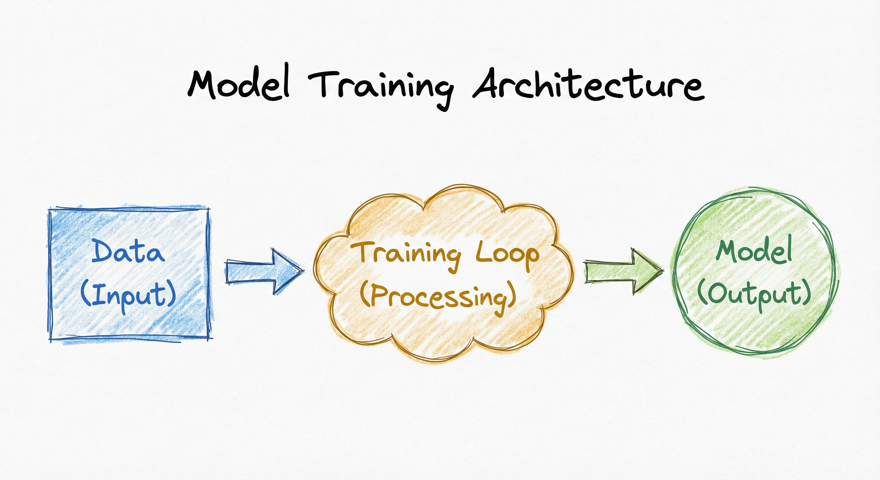
Model training is the computational heart of every machine learning system -- the phase where a model iteratively adjusts its parameters to minimize a loss function on observed data. It is where theory meets compute, and where the quality ceiling of your entire ML pipeline is established.
At its core, training is a numerical optimization problem: you feed data through a parameterized function, measure how wrong the output is, compute the gradient of that error with respect to every parameter, and nudge each parameter in the direction that reduces the error. Repeat this millions of times, and the model learns. Simple in concept, brutally complex in practice.
Why does this block matter so much in system design? Because training decisions -- batch size, learning rate schedule, optimizer choice, convergence criteria, checkpointing strategy -- cascade through everything downstream. A poorly trained model cannot be rescued by better serving infrastructure or smarter post-processing. The training phase is where you pay the compute bill, burn the GPU hours, and either build a model worth deploying or waste weeks of engineering time.
From a Bengaluru startup fine-tuning a BERT model on a single A10G to Google training Gemini across thousands of TPU v5e pods, the fundamental loop is the same. What changes is the scale, the tooling, and the budget. This guide covers it all -- from the math of backpropagation to the economics of GPU clusters in AWS Mumbai.
Concept Snapshot
- What It Is
- The iterative process of optimizing a model's parameters by minimizing a loss function over training data using gradient-based optimization.
- Category
- Model Training
- Complexity
- Intermediate
- Inputs / Outputs
- Inputs: training data, validation data, hyperparameter configuration (learning rate, batch size, epochs). Outputs: trained model weights (checkpoint), training metrics (loss curves, validation scores).
- System Placement
- Sits after data preprocessing and train/test split, and before model evaluation, model registry, and serving.
- Also Known As
- model fitting, model optimization, parameter learning, training loop, training pipeline
- Typical Users
- ML Engineers, Data Scientists, Research Scientists, MLOps Engineers
- Prerequisites
- Linear algebra (matrix operations, gradients), Calculus (chain rule, partial derivatives), Probability and statistics, Python programming, Basic understanding of neural network architectures
- Key Terms
- loss functiongradient descentbackpropagationlearning ratebatch sizeepochearly stoppingcheckpointingmixed precisiondistributed training
Why This Concept Exists
From Hand-Crafted Rules to Learned Parameters
Before machine learning, software systems encoded human expertise directly as rules. A spam filter had handwritten patterns; a recommendation engine used manually designed heuristics. Model training changed this paradigm entirely: instead of programming rules, you provide examples and let an optimization algorithm discover the patterns.
The idea is old -- the perceptron learning algorithm dates to 1958 (Frank Rosenblatt), and backpropagation was popularized in 1986 by Rumelhart, Hinton, and Williams. But for decades, training was limited by compute. You could train small models on small datasets, and that was about it.
The Deep Learning Inflection Point
Everything changed around 2012 when Alex Krizhevsky trained AlexNet on two GTX 580 GPUs and won ImageNet by a massive margin. That result proved two things: (1) deeper networks could learn richer representations, and (2) GPUs could make training these networks practical. The modern era of model training was born.
Since then, training has scaled by roughly 10x every 18 months. GPT-3 (2020) required ~3,640 petaflop-days of compute. GPT-4 (2023) is estimated at 100x that. The training infrastructure has evolved from a single GPU to warehouse-scale clusters with custom interconnects.
Why It's a Distinct System Block
In an ML system design, training is separated from serving because they have fundamentally different computational profiles:
- Training is compute-bound, batch-oriented, and latency-tolerant. You can wait hours or days for a result.
- Serving is memory-bound, request-oriented, and latency-sensitive. Every millisecond matters.
This separation is why you have a training pipeline (offline, GPU-heavy, scheduled) and a serving pipeline (online, optimized for throughput). The trained model artifact -- a checkpoint file containing learned weights -- is the bridge between these two worlds.
Key Takeaway: Model training exists because we replaced hand-crafted rules with learned parameters, and the optimization process to learn those parameters is computationally intensive enough to deserve its own dedicated infrastructure, budget, and operational strategy.
Core Intuition & Mental Model
The Training Loop as a Feedback System
Here's the simplest way to think about model training: it's a feedback loop. The model makes a prediction, you measure how wrong it was, and you adjust the model to be less wrong next time. That's it. Everything else -- fancy optimizers, learning rate schedules, distributed training -- is engineering to make this loop run faster, more reliably, and at larger scale.
Imagine you're blindfolded on a hilly landscape and trying to find the lowest valley. You can feel the slope under your feet (that's the gradient), and you take a step downhill (that's a parameter update). The size of your step is the learning rate. If you take steps that are too large, you'll overshoot the valley and bounce around. Too small, and you'll take forever to get there. The art of training is choosing the right step size and knowing when you've arrived.
Why Training Is Hard: The Loss Landscape
The reason training is non-trivial is that the loss landscape of a neural network is incredibly complex. It has billions of dimensions (one per parameter), and it's filled with saddle points, local minima, flat regions, and sharp ravines. The optimizer has to navigate all of this without a map.
This is why training is as much art as science. Two identical architectures trained with different random seeds, batch sizes, or learning rate schedules can produce models with vastly different performance. Reproducibility is a constant battle.
The Three Things That Matter Most
After years of collective experience across the ML community, three factors dominate training outcomes:
- Data quality and quantity -- no optimizer can compensate for bad data. Garbage in, garbage out.
- Learning rate schedule -- this single hyperparameter has more impact on final model quality than almost any architectural choice.
- Knowing when to stop -- training too long leads to overfitting; stopping too early leaves performance on the table. Early stopping with patience is your safety net.
Expert Note: If you're debugging a training run and don't know where to start, check these three things in order: data quality, learning rate, and overfitting. They account for 80% of training failures.
Technical Foundations
The Optimization Problem
Model training solves the following optimization problem. Given a dataset , a parameterized model , and a loss function , find the parameters that minimize the empirical risk:
where is an optional regularization term (e.g., L2 weight decay: ).
Gradient Descent
The workhorse algorithm is gradient descent. At each step , parameters are updated:
where is the learning rate. In practice, we use mini-batch stochastic gradient descent (SGD), computing the gradient over a random subset of size :
Backpropagation
The gradient is computed efficiently via backpropagation, which applies the chain rule recursively through the computational graph. For a network with layers , the gradient at layer is:
where denotes the activations at layer . This chain of multiplications is why deep networks suffer from vanishing gradients (products shrink to zero) or exploding gradients (products blow up).
The Adam Optimizer
The most widely used optimizer in modern deep learning is Adam (Adaptive Moment Estimation), which maintains per-parameter adaptive learning rates using first and second moment estimates:
with typical defaults , , .
Learning Rate Schedules
A fixed learning rate rarely works well in practice. Common schedules include:
- Cosine annealing:
- Linear warmup + decay:
- Step decay: where is the step size and is the decay factor
Convergence Criteria
Training terminates when one of these conditions is met:
- Maximum epochs reached:
- Early stopping: validation loss has not improved for consecutive evaluations (patience)
- Gradient norm falls below threshold:
- Loss plateau: for consecutive steps
Internal Architecture
A production model training system is far more than a model.fit() call. It consists of a data loading pipeline, the training loop itself, a checkpointing and experiment tracking layer, and infrastructure for distributed execution. Let's walk through the architecture.
The training loop is the inner cycle (forward pass -> loss -> backward pass -> optimizer step), wrapped by an outer loop that handles epoch management, validation, checkpointing, and early stopping. In a distributed setting, gradient synchronization (via AllReduce or parameter server) is inserted between the backward pass and the optimizer step.
The data loading pipeline runs asynchronously on CPU, prefetching and preprocessing the next batch while the GPU executes the current training step. This overlap is critical -- without it, the GPU would idle during data loading, wasting expensive compute.
Key Components
Data Loader / Sampler
Reads training data from storage (disk, object store, or distributed file system), applies shuffling and sampling strategies, and delivers mini-batches to the training loop. In PyTorch, this is DataLoader with num_workers for parallel prefetching. The sampler controls how data is partitioned across workers in distributed training (DistributedSampler).
Forward Pass Engine
Executes the model's computation graph on input data to produce predictions. In mixed precision training, this runs in FP16/BF16 for speed while maintaining an FP32 master copy of weights for numerical stability.
Loss Function
Computes the scalar loss value that measures prediction error. Common choices: cross-entropy for classification (), MSE for regression (), contrastive losses for embedding learning.
Backward Pass / Autograd
Computes gradients of the loss with respect to all trainable parameters using automatic differentiation (reverse mode). PyTorch's autograd and JAX's jax.grad handle this transparently. Memory consumption peaks during this phase because all intermediate activations must be stored.
Optimizer
Applies the gradient update rule (SGD, Adam, AdamW, LAMB, etc.) to adjust model parameters. Maintains optimizer state (momentum, variance estimates) which can be 2-3x the model size in memory for Adam-family optimizers.
Learning Rate Scheduler
Adjusts the learning rate over the course of training according to a predefined schedule (cosine annealing, linear warmup + decay, step decay, reduce-on-plateau). Interacts directly with the optimizer at each step or epoch.
Gradient Scaler (Mixed Precision)
Scales the loss before backpropagation to prevent gradient underflow in FP16 training. Unscales gradients before the optimizer step. Essential for stable mixed precision training. Implemented as torch.amp.GradScaler in PyTorch.
Checkpoint Manager
Periodically saves model weights, optimizer state, scheduler state, and training metadata to persistent storage. Enables training resumption after failures and keeps the best model based on validation performance. For large models, this can mean writing 10-100+ GB per checkpoint.
Validation Loop
Periodically evaluates the model on held-out validation data (without gradient computation) to track generalization performance. Feeds results to the early stopping logic and checkpoint manager.
Experiment Tracker
Logs hyperparameters, metrics (loss, accuracy, learning rate), system metrics (GPU utilization, memory), and artifacts (checkpoints, plots) for reproducibility and comparison. Tools: MLflow, Weights & Biases, TensorBoard.
Data Flow
Training Data Flow: Raw data is loaded from storage (S3, GCS, local disk) by the DataLoader, which applies shuffling, batching, and optional augmentation on CPU worker threads. Preprocessed mini-batches are transferred to GPU memory via pinned memory and pin_memory=True.
Compute Flow: Each mini-batch flows through the forward pass (model computation), loss computation, backward pass (gradient computation via autograd), and optimizer step (parameter update). In mixed precision, the forward and backward passes run in FP16/BF16 while the optimizer step uses FP32 master weights.
Gradient Flow (Distributed): In data-parallel distributed training, each worker computes gradients on its local batch. Gradients are synchronized across workers via AllReduce (NCCL for NVIDIA GPUs) before the optimizer step. This ensures all workers maintain identical model weights.
Metrics Flow: Training loss, validation metrics, learning rate, and system metrics are streamed to the experiment tracker. The validation loop runs periodically (every steps or every epoch) and reports validation loss to the early stopping controller.
Checkpoint Flow: The checkpoint manager saves full training state (model weights, optimizer state, epoch number, best validation score) to persistent storage at configurable intervals. On failure, training resumes from the last checkpoint with no lost progress.
A directed flow showing: Training Data Store -> Data Loader -> Preprocessing -> Forward Pass -> Loss Computation -> Backward Pass -> Optimizer Step, with a branching path to Validation Loop and Early Stopping check. The Optimizer Step also connects to a Metrics Logger and Experiment Tracker. Early Stopping leads to Save Best Checkpoint -> Model Registry.
How to Implement
The Two Paradigms: Script-Based vs. Framework-Based
Model training implementation falls into two categories:
Script-based training (raw PyTorch/TensorFlow): You write the training loop yourself, giving you full control over every detail -- gradient accumulation, custom logging, mixed precision, distributed strategy. This is the standard approach for research and custom production training.
Framework-based training (Hugging Face Trainer, PyTorch Lightning, Keras model.fit): A higher-level abstraction that handles the boilerplate -- distributed training, mixed precision, logging, checkpointing. Faster to get started, but less control over the details.
For production ML systems, the choice depends on your team's needs. If you're fine-tuning a transformer model, Hugging Face Trainer gives you 80% of what you need with 20% of the code. If you're training a custom architecture with non-standard loss functions, raw PyTorch gives you the flexibility you need.
Cost Context: A single A100 (80GB) on AWS Mumbai (ap-south-1) costs approximately 120-360/month) -- very manageable. Full pretraining of a large model, however, can run into crores of rupees.
import torch
import torch.nn as nn
from torch.utils.data import DataLoader
from torch.amp import autocast, GradScaler
import copy

def train_model(
    model: nn.Module,
    train_loader: DataLoader,
    val_loader: DataLoader,
    optimizer: torch.optim.Optimizer,
    scheduler: torch.optim.lr_scheduler._LRScheduler,
    loss_fn: nn.Module,
    num_epochs: int = 100,
    patience: int = 10,
    gradient_accumulation_steps: int = 4,
    max_grad_norm: float = 1.0,
    device: str = "cuda",
):
    scaler = GradScaler()
    best_val_loss = float("inf")
    best_model_state = None
    patience_counter = 0

    for epoch in range(num_epochs):
        # --- Training Phase ---
        model.train()
        total_train_loss = 0.0
        optimizer.zero_grad()

        for step, (inputs, targets) in enumerate(train_loader):
            inputs, targets = inputs.to(device), targets.to(device)

            with autocast(device_type="cuda", dtype=torch.float16):
                outputs = model(inputs)
                loss = loss_fn(outputs, targets)
                loss = loss / gradient_accumulation_steps

            scaler.scale(loss).backward()

            if (step + 1) % gradient_accumulation_steps == 0:
                scaler.unscale_(optimizer)
                torch.nn.utils.clip_grad_norm_(model.parameters(), max_grad_norm)
                scaler.step(optimizer)
                scaler.update()
                optimizer.zero_grad()

            total_train_loss += loss.item() * gradient_accumulation_steps

        avg_train_loss = total_train_loss / len(train_loader)
        scheduler.step()

        # --- Validation Phase ---
        model.eval()
        total_val_loss = 0.0
        with torch.no_grad():
            for inputs, targets in val_loader:
                inputs, targets = inputs.to(device), targets.to(device)
                with autocast(device_type="cuda", dtype=torch.float16):
                    outputs = model(inputs)
                    loss = loss_fn(outputs, targets)
                total_val_loss += loss.item()

        avg_val_loss = total_val_loss / len(val_loader)
        current_lr = scheduler.get_last_lr()[0]

        print(f"Epoch {epoch+1}/{num_epochs} | "
              f"Train Loss: {avg_train_loss:.4f} | "
              f"Val Loss: {avg_val_loss:.4f} | "
              f"LR: {current_lr:.2e}")

        # --- Early Stopping ---
        if avg_val_loss < best_val_loss:
            best_val_loss = avg_val_loss
            best_model_state = copy.deepcopy(model.state_dict())
            patience_counter = 0
            torch.save({
                "epoch": epoch,
                "model_state_dict": model.state_dict(),
                "optimizer_state_dict": optimizer.state_dict(),
                "scheduler_state_dict": scheduler.state_dict(),
                "best_val_loss": best_val_loss,
            }, "best_checkpoint.pt")
        else:
            patience_counter += 1
            if patience_counter >= patience:
                print(f"Early stopping at epoch {epoch+1}")
                break

    model.load_state_dict(best_model_state)
    return model
This is a production-quality training loop that includes all the essential components: mixed precision training via autocast and GradScaler for ~2x speedup on modern GPUs, gradient accumulation to simulate larger batch sizes when GPU memory is limited, gradient clipping to prevent exploding gradients, early stopping with patience to prevent overfitting, and checkpoint saving with full training state for resumability. The gradient_accumulation_steps=4 means the effective batch size is 4x the DataLoader batch size.
from transformers import (
    AutoModelForSequenceClassification,
    AutoTokenizer,
    TrainingArguments,
    Trainer,
    EarlyStoppingCallback,
)
from datasets import load_dataset
import numpy as np
from sklearn.metrics import accuracy_score, f1_score

# Load model and tokenizer
model_name = "bert-base-uncased"
tokenizer = AutoTokenizer.from_pretrained(model_name)
model = AutoModelForSequenceClassification.from_pretrained(
    model_name, num_labels=2
)

# Prepare dataset
dataset = load_dataset("imdb")
def tokenize(batch):
    return tokenizer(batch["text"], padding="max_length", truncation=True, max_length=512)

tokenized = dataset.map(tokenize, batched=True)

def compute_metrics(eval_pred):
    logits, labels = eval_pred
    preds = np.argmax(logits, axis=-1)
    return {
        "accuracy": accuracy_score(labels, preds),
        "f1": f1_score(labels, preds, average="weighted"),
    }

# Training arguments with all key settings
training_args = TrainingArguments(
    output_dir="./results",
    num_train_epochs=5,
    per_device_train_batch_size=16,
    per_device_eval_batch_size=32,
    gradient_accumulation_steps=2,      # Effective batch size = 16 * 2 = 32
    learning_rate=2e-5,
    weight_decay=0.01,
    warmup_ratio=0.1,                   # 10% warmup
    lr_scheduler_type="cosine",
    fp16=True,                          # Mixed precision
    eval_strategy="steps",
    eval_steps=500,
    save_strategy="steps",
    save_steps=500,
    save_total_limit=3,                 # Keep only 3 best checkpoints
    load_best_model_at_end=True,
    metric_for_best_model="f1",
    greater_is_better=True,
    logging_steps=100,
    report_to="wandb",                  # Log to Weights & Biases
    dataloader_num_workers=4,
    dataloader_pin_memory=True,
)

trainer = Trainer(
    model=model,
    args=training_args,
    train_dataset=tokenized["train"],
    eval_dataset=tokenized["test"],
    compute_metrics=compute_metrics,
    callbacks=[EarlyStoppingCallback(early_stopping_patience=3)],
)

trainer.train()
trainer.save_model("./final_model")
The Hugging Face Trainer abstracts away the training loop boilerplate while exposing all critical knobs. Key settings here: fp16=True enables mixed precision, gradient_accumulation_steps=2 doubles effective batch size, warmup_ratio=0.1 provides linear warmup for the first 10% of training, lr_scheduler_type='cosine' uses cosine annealing, and EarlyStoppingCallback monitors the specified metric. The save_total_limit=3 prevents disk bloat from too many checkpoints -- critical when each checkpoint is several GB.
import torch
import torch.distributed as dist
import torch.nn as nn
from torch.nn.parallel import DistributedDataParallel as DDP
from torch.utils.data import DataLoader, DistributedSampler
import os

def setup_distributed():
    dist.init_process_group(backend="nccl")
    local_rank = int(os.environ["LOCAL_RANK"])
    torch.cuda.set_device(local_rank)
    return local_rank

def train_distributed(model, train_dataset, val_dataset, num_epochs=10):
    local_rank = setup_distributed()
    device = torch.device(f"cuda:{local_rank}")

    model = model.to(device)
    model = DDP(model, device_ids=[local_rank])

    # DistributedSampler ensures each GPU gets a unique subset
    train_sampler = DistributedSampler(train_dataset, shuffle=True)
    train_loader = DataLoader(
        train_dataset,
        batch_size=32,
        sampler=train_sampler,
        num_workers=4,
        pin_memory=True,
    )

    optimizer = torch.optim.AdamW(model.parameters(), lr=3e-4)
    loss_fn = nn.CrossEntropyLoss()

    for epoch in range(num_epochs):
        train_sampler.set_epoch(epoch)  # Ensures different shuffling per epoch
        model.train()

        for batch_idx, (inputs, targets) in enumerate(train_loader):
            inputs, targets = inputs.to(device), targets.to(device)

            outputs = model(inputs)
            loss = loss_fn(outputs, targets)

            optimizer.zero_grad()
            loss.backward()  # DDP handles gradient sync via AllReduce
            optimizer.step()

        # Only save on rank 0
        if local_rank == 0:
            torch.save(model.module.state_dict(), f"checkpoint_epoch_{epoch}.pt")

    dist.destroy_process_group()

# Launch with: torchrun --nproc_per_node=4 train.py
Distributed Data Parallel (DDP) is PyTorch's recommended approach for multi-GPU training. Each GPU runs a full copy of the model on a different data subset. Gradients are synchronized via AllReduce (NCCL backend for NVIDIA GPUs) after each backward pass. Key details: DistributedSampler partitions data across GPUs, set_epoch(epoch) ensures different shuffling per epoch, and checkpoints are saved only on rank 0 to avoid duplicate writes. Note model.module.state_dict() to unwrap the DDP wrapper. Launch with torchrun which handles LOCAL_RANK environment variable setup.
# Training configuration (YAML)
model:
  architecture: bert-base-uncased
  num_labels: 2

training:
  num_epochs: 20
  batch_size: 32
  gradient_accumulation_steps: 4
  effective_batch_size: 128

  optimizer:
    name: adamw
    learning_rate: 2e-5
    weight_decay: 0.01
    betas: [0.9, 0.999]
    eps: 1e-8

  scheduler:
    name: cosine_with_warmup
    warmup_ratio: 0.1
    min_lr_ratio: 0.01

  early_stopping:
    patience: 5
    metric: val_f1
    mode: max

  mixed_precision: fp16
  gradient_clipping: 1.0

  checkpointing:
    save_every_n_steps: 500
    keep_top_k: 3
    save_optimizer_state: true

data:
  train_path: s3://my-bucket/train.parquet
  val_path: s3://my-bucket/val.parquet
  num_workers: 4
  pin_memory: true
  shuffle: true

distributed:
  strategy: ddp
  num_gpus: 4
  backend: nccl
Common Implementation Mistakes
- ●
Setting the learning rate too high or too low without a warmup: A learning rate that's too high causes divergence (loss explodes); too low leads to painfully slow convergence. Always use a warmup phase (5-10% of total steps) when training with Adam or AdamW. The warmup lets the optimizer's moment estimates stabilize before taking large steps.
- ●
Forgetting to call
model.eval()during validation: Withoutmodel.eval(), dropout and batch normalization layers remain in training mode, producing noisy and unreliable validation metrics. This is a subtle bug that can make you think your model is worse than it actually is. - ●
Not setting
train_sampler.set_epoch(epoch)in distributed training: Without this call, theDistributedSampleruses the same data partition every epoch, meaning each GPU sees the same subset repeatedly. This effectively reduces your dataset size and hurts model quality. - ●
Saving only model weights without optimizer and scheduler state: If training crashes and you resume from a weights-only checkpoint, the optimizer resets (losing momentum and variance estimates for Adam) and the learning rate schedule restarts. This can waste days of compute. Always save the full training state.
- ●
Ignoring GPU memory when choosing batch size: Picking the largest batch size that fits in GPU memory without accounting for gradient computation overhead. The backward pass requires storing intermediate activations, roughly doubling memory usage compared to inference. Use
gradient_accumulation_stepsto simulate large batch sizes instead. - ●
Training for a fixed number of epochs without early stopping: This either leads to overfitting (training too long) or underfitting (stopping too early by guessing the epoch count). Always monitor validation loss and implement early stopping with patience >= 5-10 epochs.
- ●
Not normalizing or standardizing input data: Training on unnormalized data can lead to poor convergence, especially with gradient-based optimizers. Features on vastly different scales cause the loss landscape to be poorly conditioned, making optimization harder.
When Should You Use This?
Use When
You need a model customized to your specific data distribution -- pretrained models don't capture your domain-specific patterns (e.g., training a fraud detection model on your company's transaction data)
No suitable pretrained model exists for your task, or the available models perform below your quality threshold on your evaluation set
You have sufficient labeled data (typically 1K+ examples for fine-tuning, 10K+ for training from scratch) and compute budget to run the training process
Your production requirements demand a specific model size, latency, or accuracy profile that off-the-shelf models don't meet
You need to train on proprietary or sensitive data that cannot be sent to third-party API providers for privacy or compliance reasons (common in BFSI and healthcare in India)
You want to distill a larger model into a smaller, faster model optimized for edge deployment or cost-sensitive serving
Avoid When
A pretrained model or API (GPT-4o, Claude, Gemini) already solves your problem with acceptable quality -- training your own model adds complexity, cost, and maintenance burden for no quality gain
You have fewer than 100 labeled examples -- few-shot prompting or RAG will likely outperform a fine-tuned model at this data scale
Your team lacks the ML engineering expertise to debug training issues (gradient explosion, data leakage, overfitting) -- the debugging cycle can be expensive and demoralizing
The compute budget is severely constrained and you cannot afford even a few GPU-hours -- consider using pretrained models via API or CPU-friendly models like scikit-learn
Requirements change frequently (weekly or faster) -- retraining is slow and expensive; prompt engineering or RAG-based approaches adapt much faster
You're building a prototype to validate the product idea -- invest in training only after you've confirmed the product-market fit
Key Tradeoffs
Compute Cost vs. Model Quality
More training compute generally improves model quality, but with diminishing returns. The Chinchilla scaling law (Hoffmann et al., 2022) suggests that for a given compute budget , the optimal allocation is roughly equal between model size and training data: and . Training a smaller model on more data often outperforms training a larger model on less data.
For Indian startups, this translates to a practical decision: instead of renting 8x A100s for 2 hours, you might get better results from 1x A100 for 16 hours on a larger dataset. The hourly cost in AWS Mumbai (ap-south-1) for a p4d.24xlarge (8x A100) is ~1.00 (~INR 83/hour). Spot instances can reduce this by 60-70%.
Batch Size vs. Generalization
| Batch Size | Pros | Cons |
|---|---|---|
| Small (8-32) | Better generalization, lower memory | Noisy gradients, slower wall-clock time |
| Medium (64-256) | Good balance of speed and generalization | Requires gradient accumulation on single GPU |
| Large (512-4096) | Fast convergence, full GPU utilization | May hurt generalization, requires LR warmup |
The relationship between batch size and learning rate is roughly linear: when you double the batch size, double the learning rate. This is the linear scaling rule from Goyal et al. (2017).
Training From Scratch vs. Fine-Tuning
| Approach | Data Needed | Compute Cost | Quality |
|---|---|---|---|
| Train from scratch | 100K-1B+ examples | Very high (days-weeks on multiple GPUs) | Highest potential if data is sufficient |
| Full fine-tuning | 1K-100K examples | Medium (hours on single GPU) | Very good for most tasks |
| LoRA / QLoRA | 1K-10K examples | Low (minutes-hours on single GPU) | Good, ~95-99% of full fine-tuning |
| Prompt tuning | 100-1K examples | Very low | Adequate for simple tasks |
Rule of Thumb for Indian Startups: Start with LoRA fine-tuning of an open-source model (Llama 3, Mistral). Budget INR 5,000-20,000/month for training compute on AWS/GCP spot instances. Only invest in full fine-tuning or pretraining once you've validated the use case and have a clear quality gap.
Alternatives & Comparisons
Full fine-tuning updates all model parameters, while the generic 'model training' block encompasses training from scratch as well. Fine-tuning is preferred when you have a strong pretrained foundation and limited task-specific data. Training from scratch is necessary when no relevant pretrained model exists or when your data distribution is fundamentally different from anything in pretraining corpora.
LoRA adds small trainable rank-decomposition matrices while freezing the base model, requiring 10-100x less GPU memory than full training. Choose LoRA when you have limited compute or need to maintain multiple task-specific adapters. Choose full model training when you need maximum quality and have sufficient compute budget.
Distillation trains a smaller 'student' model to mimic a larger 'teacher' model's outputs. It's an alternative to training a large model when you need deployment efficiency. Choose distillation when you have a strong teacher model and need a faster/smaller production model. Choose direct training when no suitable teacher exists.
Hyperparameter tuning is a meta-layer on top of model training -- it runs multiple training experiments with different configurations to find optimal settings. It's not an alternative to training but a companion. Use automated HPO (Optuna, Ray Tune) when you have the compute budget for 10-100+ trial runs.
Pros, Cons & Tradeoffs
Advantages
Custom models for your data -- training produces a model tailored to your specific data distribution, capturing domain-specific patterns that pretrained models miss. A fraud detection model trained on your bank's transaction data will outperform a general-purpose model every time.
Full control over the model lifecycle -- you control architecture, training data, optimization strategy, and deployment. No dependency on third-party API providers, no usage-based pricing surprises, and full data privacy.
Scalable performance improvement -- as you collect more data, you can retrain to continuously improve model quality. The virtuous cycle of data -> training -> deployment -> more data is the engine of production ML systems.
Cost-effective at scale -- for high-throughput serving (millions of predictions/day), a self-trained model running on your infrastructure is dramatically cheaper than API calls. A fine-tuned 7B model serving at 1M requests/day costs ~INR 50,000/month on a single A10G, vs. INR 5-15 lakh/month for equivalent GPT-4o API calls.
Intellectual property -- the trained model weights are your IP. You can deploy them anywhere without licensing constraints (depending on the base model license), sell model-powered products, and build competitive moats.
Enables edge deployment -- only by training (or distilling) your own model can you deploy to resource-constrained environments like mobile devices, IoT, or regions with poor internet connectivity -- relevant for India's tier-2 and tier-3 cities.
Disadvantages
High upfront compute cost -- GPU time is expensive, especially for large models. Training a 70B parameter model from scratch can cost $500K+ (~INR 4.2 crore). Even fine-tuning a 7B model requires several hours of A100 time. For resource-constrained Indian startups, this can be a significant barrier.
Requires significant ML engineering expertise -- debugging training issues (divergence, overfitting, data leakage, gradient problems) requires deep knowledge. Hiring experienced ML engineers in India costs INR 25-60 lakh/year, and the talent pool is competitive.
Slow iteration cycle -- each training experiment takes hours to days. Unlike prompt engineering where you can iterate in minutes, training experiments have a long feedback loop that slows down product development.
Data dependency -- training quality is bounded by data quality and quantity. Collecting, cleaning, and labeling high-quality training data is often more expensive and time-consuming than the training itself.
Reproducibility challenges -- non-determinism in GPU operations, data shuffling, and floating-point arithmetic means that two identical training runs can produce slightly different models. This makes debugging and auditing difficult.
Ongoing maintenance burden -- models degrade over time as the data distribution shifts (concept drift). You need continuous retraining pipelines, monitoring, and alerting -- this is operational overhead that lasts as long as the model is in production.
Failure Modes & Debugging
Training divergence (loss explosion)
Cause
Learning rate too high, unstable loss function, or corrupted training data causing extreme gradient values. In mixed precision training, this can also happen when the gradient scaler fails to prevent FP16 underflow/overflow.
Symptoms
Training loss suddenly spikes to NaN or inf. Gradient norms explode to very large values. In TensorBoard/W&B, you'll see the loss curve shoot upward and then flatline at NaN. The model outputs garbage predictions.
Mitigation
Reduce the learning rate by 2-10x. Add gradient clipping (max_grad_norm=1.0). Use learning rate warmup for the first 5-10% of training steps. In mixed precision, ensure GradScaler is properly configured. Check training data for outliers or corrupted samples. Monitor gradient norms -- if they exceed 10-100x their typical range, something is wrong.
Overfitting
Cause
Model capacity exceeds what the training data can support. Insufficient regularization, training for too many epochs, or data leakage between train and validation sets.
Symptoms
Training loss continues to decrease while validation loss plateaus or increases. The gap between training and validation metrics grows over epochs. The model memorizes training examples rather than learning generalizable patterns -- performance on unseen data is poor.
Mitigation
Implement early stopping with patience (monitor validation loss, stop when it hasn't improved for N epochs). Add regularization: weight decay (L2), dropout, data augmentation. Reduce model capacity if feasible. Increase training data volume. Check for data leakage -- this is surprisingly common and can completely invalidate your results.
Underfitting / slow convergence
Cause
Learning rate too low, model capacity too small for the task, insufficient training data, or poor data preprocessing (unnormalized features, missing values).
Symptoms
Both training and validation loss remain high and plateau early. The model performs barely better than a random baseline. Training appears to converge but at an unacceptably high loss value.
Mitigation
Increase the learning rate (try 3-10x). Use a larger model or add more layers. Ensure data is properly preprocessed and normalized. Try a different optimizer (switch from SGD to AdamW). Verify that the loss function matches your task (e.g., don't use MSE for classification). Check that labels are correct -- mislabeled data is more common than you'd think.
GPU out-of-memory (OOM)
Cause
Batch size too large, model too large for available VRAM, or memory leak from accumulated computation graphs (forgetting torch.no_grad() during validation, not detaching tensors).
Symptoms
CUDA OOM error during training. On shared GPU clusters, the job gets killed by the OOM killer. Memory usage grows linearly across training steps instead of staying constant (indicates a memory leak).
Mitigation
Reduce batch size and use gradient accumulation to maintain effective batch size. Enable mixed precision training (halves activation memory). Use gradient checkpointing (torch.utils.checkpoint) to trade compute for memory. For large models, consider FSDP (Fully Sharded Data Parallel) or DeepSpeed ZeRO. Always wrap validation in torch.no_grad(). Profile memory with torch.cuda.memory_summary().
Data leakage
Cause
Information from the validation or test set leaks into training, either through improper splitting (e.g., splitting rows instead of users/sessions), feature engineering using future data, or preprocessing fitted on the full dataset before splitting.
Symptoms
Suspiciously high validation/test metrics that don't translate to production performance. The model appears excellent in offline evaluation but performs poorly when deployed. If validation accuracy is 99%+ on a task where 90% would be state-of-the-art, you almost certainly have leakage.
Mitigation
Split data before any preprocessing or feature engineering. Use temporal splits for time-series data (train on past, validate on future). For user-level data, split by user ID, not by individual records. Audit the feature engineering pipeline for any use of future information. Run a baseline model -- if a simple logistic regression achieves near-perfect accuracy, something is leaking.
Checkpoint corruption / loss
Cause
Training job killed during checkpoint write (spot instance preemption, OOM kill, network failure). Disk full, or storage quota exceeded on cloud storage. No checkpoint retention policy leading to overwritten checkpoints.
Symptoms
Training resumption fails with corrupted checkpoint error. Best model weights are lost after a crash. In distributed training, inconsistent checkpoint state across workers.
Mitigation
Use atomic writes (write to temp file, then rename). Implement checkpoint validation (load and verify after save). Save to persistent storage (S3, GCS) in addition to local disk. Keep at least 2-3 recent checkpoints (save_total_limit). For spot instances, checkpoint more frequently (every 15-30 minutes) and use spot instance interruption warnings to trigger an emergency save.
Vanishing / exploding gradients
Cause
Poor weight initialization, very deep networks without skip connections, or activation functions with saturating gradients (sigmoid, tanh). The chain of multiplications in backpropagation either shrinks gradients to zero (vanishing) or amplifies them to infinity (exploding).
Symptoms
Vanishing: early layers stop learning, loss plateaus, gradient norms near zero for early layers. Exploding: NaN loss, wildly oscillating loss curve, very large gradient norms. Both can appear as mysteriously poor training despite a correct setup.
Mitigation
Use residual connections (ResNet-style skip connections). Choose ReLU or GELU activations over sigmoid/tanh. Apply proper weight initialization (He initialization for ReLU, Xavier for tanh). Use gradient clipping for exploding gradients. Layer normalization or batch normalization stabilizes the gradient flow. For transformers, pre-norm architecture (LayerNorm before attention) is more stable than post-norm.
Placement in an ML System
Training's Place in the ML System
Model training sits squarely in the offline pipeline of an ML system. It consumes preprocessed, validated training data from upstream and produces trained model artifacts (checkpoints) for downstream consumption by the model registry and serving infrastructure.
The training pipeline is typically orchestrated as a scheduled or triggered workflow. In mature organizations, it runs on dedicated GPU infrastructure (on-prem clusters or cloud GPU instances) separate from the serving infrastructure. This separation is essential because training workloads are bursty (you run them when new data is available or when a model refresh is needed) while serving workloads are continuous.
In a typical production setup:
- Data pipeline prepares and validates training data (upstream:
data-validation,feature-store) - Training pipeline runs model training with hyperparameter tuning (this block +
hyperparameter-tuning) - Evaluation pipeline validates the trained model against quality thresholds (
accuracy-metric,cross-validation) - Deployment pipeline registers the approved model and pushes it to serving (downstream:
model-registry,model-serving)
The handoff between training and serving is mediated by the model registry, which versions trained artifacts and tracks metadata (training data snapshot, hyperparameters, evaluation metrics). This is the boundary between the offline training world and the online serving world.
Key Insight: Training is an offline, GPU-intensive process that produces the model artifact. Everything it interacts with upstream is about data quality; everything downstream is about model deployment and monitoring. The quality of training directly determines the quality ceiling of the entire serving pipeline.
Pipeline Stage
Training / Offline
Upstream
- train-test-split
- feature-store
- data-validation
- data-transformation
Downstream
- model-registry
- model-serving
- accuracy-metric
- hyperparameter-tuning
Scaling Bottlenecks
Model training is fundamentally compute-bound. The bottleneck is almost always GPU throughput -- how many floating-point operations per second your hardware can sustain. A single A100 delivers ~312 TFLOPS (FP16), and training a 7B model requires ~ FLOPs, meaning roughly 1 hour of full-utilization A100 time.
At larger scales, the bottleneck shifts to inter-GPU communication. In data-parallel training across 8+ GPUs, AllReduce gradient synchronization can consume 20-40% of total training time, especially when the gradient payload is large (hundreds of MB per sync). NCCL over NVLink helps (600 GB/s), but cross-node communication over InfiniBand (400 Gbps) is still a significant overhead.
Data I/O becomes the bottleneck when training on very large datasets (terabytes) stored on networked storage. If the data pipeline can't feed the GPU fast enough, you'll see GPU utilization drop below 50%. Mitigation: use multiple DataLoader workers, pin memory, prefetch batches, and store data in efficient formats (WebDataset, TFRecord, Parquet).
Some concrete scaling numbers:
- 1x A10G: fine-tune a 1-3B model, ~$1/hour (~INR 83/hour) on AWS Mumbai
- 1x A100 (80GB): fine-tune a 7-13B model, ~$4/hour (~INR 333/hour)
- 8x A100 (p4d.24xlarge): full fine-tune a 70B model, ~$33/hour (~INR 2,750/hour)
- 64x H100 (8x p5.48xlarge): pretrain a large model, ~$300/hour (~INR 25,000/hour)
Production Case Studies
The Chinchilla paper demonstrated that most large language models were significantly undertrained relative to their size. By training a 70B parameter model (Chinchilla) on 4x more data than the 280B Gopher model, they achieved better performance with 4x less compute at inference. This fundamentally changed how the industry thinks about the compute-optimal allocation between model size and training data.
Chinchilla (70B, trained on 1.4T tokens) outperformed Gopher (280B, trained on 300B tokens) on most benchmarks while requiring 3-4x less inference compute. This paper directly influenced the training recipes of Llama 2, Mistral, and virtually every subsequent LLM.
Meta's Llama 2 paper provides one of the most detailed public accounts of large-scale model training. They trained 7B, 13B, and 70B parameter models on 2 trillion tokens using 2,048 A100 GPUs. The paper details their distributed training setup (FSDP), training stability interventions (learning rate adjustments to recover from loss spikes), and the progression from pretraining to supervised fine-tuning to RLHF.
Llama 2 70B matched or exceeded GPT-3.5 on most benchmarks while being open-source. The 70B model required approximately 1,720,320 GPU-hours of A100 compute (~$5.4M USD / ~INR 45 crore at on-demand pricing). The training recipe became the template for dozens of open-source model efforts worldwide.
Flipkart trains custom models for product search ranking, recommendation, and pricing optimization. Their training infrastructure handles models that must be retrained daily on fresh user interaction data. They use a feature store to ensure training-serving consistency and employ incremental/online learning techniques to keep models fresh without full retraining. The system processes billions of user events from 400M+ registered users.
Daily model retraining improved search relevance metrics by 12-15% compared to weekly retraining cadence. The feature store reduced training-serving skew bugs by over 80%, and the automated training pipeline reduced model refresh time from days to hours.
Zerodha, India's largest stock broker (processing 15M+ orders/day), uses trained ML models for fraud detection, order pattern analysis, and risk management. Given the regulatory sensitivity of financial models in India (SEBI compliance), they maintain strict training reproducibility, model versioning, and audit trails. Their training pipeline runs on cost-optimized infrastructure, reflecting the capital-efficient culture common in Indian fintech.
ML-based fraud detection models trained on proprietary order data reduced false positive rates by approximately 40% compared to rule-based systems, while maintaining near-zero false negative rates -- critical for regulatory compliance with SEBI norms.
Oda, a Norwegian online grocery company, trained a gradient-boosted model to predict driver non-driving time (service time at each delivery stop). Starting from zero ML capability, they built training data from GPS telemetry, order metadata, and building information. The model learns patterns like apartment buildings requiring more service time than houses, and heavy orders taking longer to unload (2021-2022).
The trained model reduced service time prediction error by 35% compared to the flat-average baseline. This directly improved route scheduling, enabling Oda to fit more deliveries per route while maintaining on-time delivery guarantees.
Zynga applied Deep Reinforcement Learning (Deep RL) in production to personalize push notification timing for mobile game players. Rather than sending notifications at fixed times, they trained a Deep Q-Network (DQN) agent that learns the optimal time to notify each user to maximize re-engagement. The state space includes user activity patterns, game progress, time since last session, and notification history (2020).
The Deep RL-based notification system improved user re-engagement by 7% over the previous heuristic-based approach. The model learns individualized optimal timing, accounting for user fatigue and session patterns — a significant improvement over one-size-fits-all scheduling.
Tooling & Ecosystem
The dominant framework for model training in both research and production. Provides autograd for automatic differentiation, torch.nn for model building, distributed training via DDP and FSDP, and mixed precision via torch.amp. The default choice for >80% of new ML projects.
High-level training abstraction for transformer models. Handles distributed training, mixed precision, gradient accumulation, logging, and checkpointing out of the box. The fastest path from pretrained model to fine-tuned model for NLP tasks.
Microsoft's library for efficient large-scale model training. ZeRO optimizer stages (1/2/3) partition optimizer state, gradients, and parameters across GPUs, enabling training of models that don't fit on a single GPU. Essential for training 13B+ parameter models.
Structured framework that organizes PyTorch training code into reusable modules. Handles distributed training, mixed precision, logging, and checkpointing with minimal boilerplate. Good middle ground between raw PyTorch and Hugging Face Trainer.
Experiment tracking platform that logs metrics, hyperparameters, system metrics, and artifacts. Provides dashboards for comparing training runs, hyperparameter sweep management, and model versioning. The de facto standard for experiment tracking.
Bayesian hyperparameter optimization framework. Automatically searches for optimal learning rate, batch size, architecture choices, etc. using Tree-structured Parzen Estimator (TPE) or CMA-ES. Integrates with PyTorch, TensorFlow, and most ML frameworks.
NVIDIA Collective Communications Library -- the communication backend for distributed GPU training. Implements AllReduce, AllGather, and other collective operations optimized for NVLink and InfiniBand interconnects. Used by PyTorch DDP and FSDP under the hood.
Open-source platform for the ML lifecycle including experiment tracking, model packaging, and model registry. Particularly popular in enterprises and teams that want a self-hosted alternative to Weights & Biases.
Research & References
Rumelhart, Hinton & Williams (1986)Nature, Vol. 323
The foundational paper that popularized backpropagation for training multi-layer neural networks. Showed that gradient descent with the chain rule could learn useful internal representations, enabling networks deeper than a single layer.
Kingma & Ba (2015)ICLR 2015
Introduced the Adam optimizer which combines adaptive learning rates with momentum. Adam maintains per-parameter learning rates using running estimates of first and second moments of the gradient. With 120K+ citations, it's the most widely used optimizer in deep learning.
Loshchilov & Hutter (2019)ICLR 2019
Introduced AdamW, which fixes a subtle bug in Adam's implementation of L2 regularization. By decoupling weight decay from the adaptive learning rate, AdamW achieves better generalization. Now the default optimizer for transformer training.
Hoffmann, Borgeaud, Mensch et al. (2022)NeurIPS 2022
The Chinchilla scaling law paper. Showed that for a given compute budget, model size and training data should be scaled equally. Proved that most existing LLMs were undertrained, shifting the field toward longer training on more data rather than simply increasing model size.
Micikevicius, Narang, Alben et al. (2018)ICLR 2018
Demonstrated that neural networks can be trained with half-precision (FP16) floating point with minimal quality loss by using loss scaling and maintaining FP32 master weights. This technique roughly doubles training throughput and halves memory usage on modern GPUs.
Goyal, Dollar, Girshick et al. (2017)arXiv preprint (Meta AI)
Established the linear scaling rule for learning rates: when batch size is multiplied by , multiply the learning rate by . Combined with gradual warmup, this enabled training ResNet-50 on ImageNet in 1 hour using 256 GPUs -- a landmark result for distributed training.
Rajbhandari, Rasley, Ruwase & He (2020)SC 2020
Introduced the ZeRO (Zero Redundancy Optimizer) technique that partitions optimizer states, gradients, and parameters across data-parallel workers. ZeRO-3 enables training models up to 1T parameters with near-linear scaling efficiency. Forms the basis of Microsoft's DeepSpeed library.
Srivastava, Hinton, Krizhevsky, Sutskever & Salakhutdinov (2014)JMLR, Vol. 15
Introduced dropout regularization, where random neurons are deactivated during training to prevent co-adaptation and reduce overfitting. Dropout remains one of the most effective and widely used regularization techniques, especially in fully connected and recurrent layers.
Interview & Evaluation Perspective
Common Interview Questions
- ●
Walk me through the model training loop. What happens at each step?
- ●
How would you handle a situation where training loss is decreasing but validation loss is increasing?
- ●
Explain the tradeoffs between different batch sizes. How do you choose the right batch size?
- ●
How does distributed training work? What's the difference between data parallel and model parallel?
- ●
What is mixed precision training and why does it help?
- ●
How do you decide between training from scratch, fine-tuning, and using LoRA?
- ●
Your training run on 4 GPUs is only 2x faster than on 1 GPU. What could be wrong?
- ●
How would you design a training pipeline that needs to retrain daily on fresh data for a recommendation system?
Key Points to Mention
- ●
The training loop has four phases: forward pass, loss computation, backward pass (backpropagation), and optimizer step. Everything else (mixed precision, gradient accumulation, distributed sync) wraps around this core.
- ●
Learning rate is the single most impactful hyperparameter. Always use warmup (5-10% of total steps) and a schedule (cosine annealing is a safe default). The linear scaling rule links batch size to learning rate.
- ●
Early stopping with patience is essential for preventing overfitting. Monitor validation loss, not training loss. Save checkpoints based on best validation metric, not latest epoch.
- ●
Mixed precision (FP16/BF16) gives ~2x speedup and ~50% memory reduction with negligible quality impact. Use
GradScalerfor FP16 stability. BF16 on Ampere+ GPUs (A100, H100) doesn't need a scaler. - ●
Gradient accumulation lets you simulate larger batch sizes without more GPU memory. Effective batch size = per-GPU batch size x accumulation steps x number of GPUs.
- ●
In distributed training, DDP (DistributedDataParallel) is the standard for multi-GPU. FSDP or DeepSpeed ZeRO for models that don't fit on a single GPU. Communication overhead is the main scaling bottleneck.
Pitfalls to Avoid
- ●
Claiming 'more epochs always means better model' -- without early stopping, more epochs leads to overfitting, not improvement. Always discuss validation-based stopping.
- ●
Confusing data parallelism with model parallelism. Data parallelism replicates the model across GPUs with different data shards. Model parallelism splits the model across GPUs. Know when each is appropriate.
- ●
Ignoring the compute cost dimension. A senior candidate should be able to estimate training cost: FLOPs = 6 x model_params x training_tokens (for transformers), then divide by GPU TFLOPS to get time.
- ●
Treating training as a one-time activity. In production, models need retraining (daily, weekly, monthly) as data distributions shift. Discuss the automation and orchestration of retraining pipelines.
- ●
Not mentioning reproducibility. Set random seeds, log all hyperparameters, version training data, and save the full training configuration alongside the checkpoint.
Senior-Level Expectation
A senior/staff-level candidate should discuss model training from both the algorithmic and systems perspective. Algorithmically: optimizer choice and tuning, learning rate schedules, convergence diagnostics, regularization strategy. Systems-wise: distributed training architecture (DDP vs. FSDP vs. DeepSpeed ZeRO), GPU memory profiling, data pipeline optimization (avoiding GPU starvation), checkpoint management, and cost estimation. They should be able to estimate training cost for a given model size and dataset (using the 6ND rule for transformers), discuss Chinchilla-optimal training, and design a complete retraining pipeline with A/B testing against the current production model. Experience with training failure debugging -- loss spikes, NaN gradients, OOM errors -- and the ability to discuss mitigation strategies with real examples separates exceptional candidates from good ones.
Summary
Let's recap what we've covered in this comprehensive guide to model training:
-
Model training is the iterative optimization of model parameters by minimizing a loss function via gradient descent and backpropagation. The training loop (forward pass -> loss -> backward pass -> optimizer step) is the computational core, wrapped by data loading, validation, checkpointing, and early stopping logic. The fundamental math is the same whether you're training a logistic regression on a laptop or a 70B transformer on a GPU cluster.
-
The critical decisions are: learning rate (always use warmup + cosine schedule), batch size (larger isn't always better -- use gradient accumulation to decouple batch size from memory), optimizer (AdamW is the default for transformers), and when to stop (early stopping with patience, not fixed epochs). Mixed precision training gives a free ~2x speedup with negligible quality impact and should be used whenever your hardware supports it.
-
Distributed training (DDP, FSDP, DeepSpeed ZeRO) enables scaling to models that don't fit on a single GPU and datasets that would take prohibitively long on one machine. The main overhead is gradient synchronization, which can consume 20-40% of training time at scale. For most teams, DDP handles multi-GPU fine-tuning well; switch to FSDP or DeepSpeed when the model exceeds single-GPU memory.
-
For Indian startups and teams, the practical playbook is: start with LoRA fine-tuning of open-source models on spot GPU instances (INR 5,000-20,000/month), implement robust checkpointing for spot interruption resilience, use experiment tracking (W&B, MLflow) from day one, and only invest in full pretraining once you've validated the use case. The economics of GPU training are favorable for India's cost-sensitive environment -- a fine-tuned 7B model serving millions of requests costs a fraction of equivalent API calls.
Model training is where compute meets data to produce intelligence. Every design decision in training -- from the choice of loss function to the checkpoint frequency -- cascades through the rest of the ML system. A well-trained model is the foundation; everything downstream can only be as good as the weights that training produces.