Drift Detection in Machine Learning
Here is a truth that every ML engineer learns the hard way: a model that works today will not work tomorrow. Not because the code changed, not because the infrastructure failed, but because the world moved on while the model stayed frozen. That slow, silent divergence between what a model learned and what reality now looks like is called drift, and detecting it before it causes damage is one of the hardest operational problems in production ML.
Drift detection is the practice of continuously monitoring the statistical properties of incoming data, model predictions, and target distributions to identify when they deviate significantly from what the model was trained on. It sits at the heart of ML observability -- the early warning system that tells you your model is losing its grip on reality.
Why does this matter so much? Because ML models are not self-correcting. A software bug crashes loudly and triggers an alert. A drifting model degrades silently -- prediction quality erodes by 0.1% per day, revenue leaks by a few basis points per week, and by the time someone notices, you have lost lakhs of rupees and months of user trust. From Flipkart's recommendation engine during seasonal shopping spikes to Razorpay's fraud detection adapting to new payment patterns, drift detection is the difference between proactive ML operations and firefighting.
In this guide, we will cover the three types of drift (data, concept, and prediction), the statistical tests that detect them, production architectures for windowed monitoring, severity thresholds, automated retraining triggers, and the tools that make all of this practical.
Concept Snapshot
- What It Is
- A monitoring technique that uses statistical tests to identify when the distribution of input features, model predictions, or the relationship between inputs and targets has shifted significantly from the training or reference distribution.
- Category
- Monitoring
- Complexity
- Intermediate
- Inputs / Outputs
- Inputs: reference (training/baseline) data distribution + current (production) data distribution. Outputs: drift scores, p-values, boolean drift alerts, and severity classifications.
- System Placement
- Sits downstream of model serving and upstream of alerting and retraining pipelines in the ML monitoring stack.
- Also Known As
- distribution shift detection, covariate shift detection, dataset shift monitoring, model decay detection, data quality monitoring
- Typical Users
- ML Engineers, MLOps Engineers, Data Scientists, Platform Engineers, Site Reliability Engineers (SREs)
- Prerequisites
- Basic probability and statistics (distributions, hypothesis testing), Model serving and inference pipelines, Feature engineering concepts, ML evaluation metrics
- Key Terms
- data driftconcept driftprediction driftcovariate shiftKS testPSIWasserstein distancereference windowanalysis windowdrift threshold
Why This Concept Exists
The Silent Failure Problem
Traditional software systems fail in observable ways: a null pointer throws an exception, a timeout triggers a circuit breaker, a disk fills up and the process exits. These failures are loud -- they show up in logs, dashboards, and on-call pages within seconds.
ML models fail differently. They fail silently. A fraud detection model trained on pre-UPI transaction patterns will happily continue scoring every transaction after UPI adoption explodes across India -- it just scores them wrong. No exception, no crash, no error log. The model's confidence scores look perfectly normal; it is the relationship between those scores and actual fraud that has broken.
This asymmetry between model confidence and model correctness is the fundamental reason drift detection exists.
The Three Forces That Cause Drift
Drift is not a single phenomenon. Three distinct forces can push a model out of alignment:
Force 1: The input distribution changes (Data Drift). User demographics shift, new product categories appear, seasonal patterns alter feature distributions. During Diwali, Flipkart's traffic patterns look nothing like a regular Tuesday in March -- feature distributions for search queries, price ranges, and category clicks all shift dramatically. A model trained on "average" patterns will struggle.
Force 2: The relationship between inputs and outputs changes (Concept Drift). Even if the features look the same, what constitutes a positive outcome may change. A spam classifier trained in 2023 encounters new social engineering tactics in 2025. The words in emails look similar, but what makes an email spam has changed. In the Indian fintech space, Razorpay's fraud models face this constantly as scammers evolve their tactics while transaction features remain superficially similar.
Force 3: The model's prediction distribution shifts (Prediction Drift). Sometimes the input data looks fine, but the model starts producing different prediction distributions -- more conservative scores, a different class balance, or shifted confidence intervals. This can indicate internal model issues or subtle upstream data quality problems.
From Manual Checks to Automated Detection
In the early days of ML operations (roughly 2015-2019), drift detection was a manual process: a data scientist would periodically pull production data, compare histograms against training data, and eyeball whether anything looked off. This worked for teams running a handful of models with weekly retraining cycles.
But modern ML platforms run hundreds or thousands of models, each processing millions of predictions daily. Swiggy alone runs recommendation, ETA prediction, search ranking, and fraud detection models simultaneously -- each with different feature sets, different drift profiles, and different tolerance thresholds. Manual inspection does not scale.
The evolution from manual to automated drift detection was driven by three catalysts: (1) the scale of model deployment outpaced human monitoring capacity, (2) research in statistical two-sample testing matured (the KS test, MMD, and Wasserstein distance became standard tools), and (3) open-source libraries like Evidently AI and NannyML made these techniques accessible without PhD-level statistics knowledge.
Key Takeaway: Drift detection exists because ML models fail silently, the world changes continuously, and humans cannot manually monitor every feature of every model at production scale.
Core Intuition & Mental Model
The Canary in the Coal Mine
Think of drift detection like the canary that coal miners used to carry underground. The canary does not fix the toxic gas -- it does not even understand chemistry. But it is exquisitely sensitive to environmental changes. When the canary shows distress, the miners know something has shifted in their environment, even if they cannot yet see it.
Drift detection is your canary. It does not tell you why the model is degrading or how to fix it. It tells you that something has changed, and it tells you fast enough to act before the consequences compound.
A Simple Mental Model: Two Jars of Marbles
Imagine you have two jars of marbles. Jar A (your reference distribution) contains the marbles you trained your model on -- 50% red, 30% blue, 20% green. Jar B (your production distribution) is what you are seeing right now.
Every hour, you draw a sample from Jar B and compare it to Jar A. If Jar B suddenly has 40% red and 40% blue, something has changed. The statistical tests we will discuss (KS, PSI, Wasserstein) are just formal ways of answering: "Are these two jars still the same?"
The tricky part is not the comparison itself -- it is deciding how different is too different. A 1% shift in marble proportions might be noise. A 15% shift is probably real. Setting that threshold correctly is where the art meets the science, and getting it wrong in either direction is costly: too sensitive and you drown in false alarms, too lenient and you miss real drift.
Why Not Just Monitor Accuracy?
Here is a question I hear constantly: "Why bother with drift detection? Why not just monitor the model's accuracy and retrain when it drops?" The answer is labels arrive late -- often very late. For Swiggy's delivery time prediction model, you know the actual delivery time within an hour. But for a credit scoring model at a bank, you will not know if the loan defaulted for 6-12 months. For Zerodha's customer churn prediction, true churn might take quarters to confirm.
Drift detection gives you a leading indicator of model degradation. It says "your input distribution has shifted significantly" weeks or months before you have the ground truth labels to confirm that accuracy has actually dropped. That early warning is worth its weight in gold.
Technical Foundations
Mathematical Framework for Drift Detection
Let us formalize the three types of drift. Suppose we have a model trained on a joint distribution . At serving time, the production joint distribution is .
Data Drift (Covariate Shift): The marginal input distribution changes while the conditional remains stable:
Concept Drift: The conditional relationship between inputs and targets changes:
This can occur even when -- the inputs look the same but the correct answers have changed.
Prediction Drift: The model's output distribution shifts:
where .
Key Statistical Tests
Kolmogorov-Smirnov (KS) Test: Compares the empirical cumulative distribution functions (ECDFs) of two samples. The test statistic is the maximum absolute difference:
where and are the ECDFs of the reference and production samples. Under the null hypothesis (no drift), the KS statistic follows a known distribution, yielding a p-value. Reject when (typically ). The KS test works for continuous univariate features.
Population Stability Index (PSI): Widely used in finance and credit scoring, PSI bins the feature values and compares the proportion in each bin:
where is the proportion of production data in bin , is the proportion of reference data in bin , and is the number of bins. Industry convention: PSI < 0.1 indicates no significant drift, 0.1-0.25 indicates moderate drift, and PSI > 0.25 indicates significant drift requiring investigation.
Wasserstein Distance (Earth Mover's Distance): Measures the minimum cost of transforming one distribution into another:
Unlike the KS test, the Wasserstein distance accounts for the magnitude of the shift, not just its existence. A distribution that shifts by 100 units scores higher than one that shifts by 1 unit, even if both are statistically significant under KS.
Jensen-Shannon Divergence (JSD): A symmetric version of KL divergence, bounded between 0 and 1:
where and is the Kullback-Leibler divergence.
Chi-Squared Test: For categorical features, compares observed vs. expected frequencies:
where is the observed frequency and is the expected frequency based on the reference distribution.
Multivariate Drift Detection
Univariate tests detect drift feature-by-feature, but subtle multivariate shifts can go undetected. The Maximum Mean Discrepancy (MMD) test addresses this:
where is a kernel function (typically RBF), and . MMD captures distributional differences in the joint feature space that per-feature tests would miss.
Practical Note: In production, you typically run univariate tests on all features as a first pass (fast, interpretable) and reserve MMD for periodic deep checks or when univariate tests disagree (some features drift, others do not).
Internal Architecture
A production drift detection system operates as a continuous monitoring loop with four main stages: data collection from the serving pipeline, windowed aggregation of statistics, statistical testing against a reference baseline, and alert routing based on severity thresholds. The architecture must handle high-throughput inference streams (potentially millions of predictions per day) while keeping compute costs manageable.
The critical design decision is windowing strategy: how much production data do you accumulate before running a drift test? Too small a window gives noisy, unreliable results (high false positive rate). Too large a window delays detection, defeating the purpose. Most production systems use sliding or tumbling windows of 1-24 hours, with the exact size tuned to the volume of traffic and the acceptable detection latency.
The architecture is deliberately decoupled: the feature logger operates asynchronously (it must not add latency to the serving path), the window aggregator batches data for efficiency, and the drift calculator runs on a schedule (every hour, every window close) rather than per-prediction. This separation ensures drift detection does not become a bottleneck in the inference pipeline.
Key Components
Feature Logger
Captures input features, model predictions, and (when available) ground truth labels from the serving pipeline. Operates asynchronously via message queues (Kafka, SQS) to avoid adding latency to inference. Logs are typically written to a time-partitioned store (S3, BigQuery, or a feature store) for downstream processing.
Reference Baseline Store
Stores the statistical profile of the reference distribution -- typically computed from the training set or a validated production window. Contains per-feature histograms, summary statistics (mean, variance, quantiles), and pre-computed distribution parameters. Updated when models are retrained. This is the 'ground truth' that production data is compared against.
Window Aggregator
Accumulates incoming feature logs into analysis windows (tumbling or sliding). Computes per-window statistics: histograms, means, quantile sketches, null rates, and cardinality counts. Uses approximate data structures (t-digest, HyperLogLog) for memory-efficient streaming aggregation at scale.
Drift Calculator
The core statistical engine. For each analysis window, runs configured statistical tests (KS, PSI, Wasserstein, chi-squared, MMD) comparing the window's distribution against the reference baseline. Outputs raw drift scores and p-values per feature.
Severity Classifier
Translates raw drift scores into actionable severity levels (none, low, medium, high, critical) based on configurable thresholds. Applies business logic: some features are more critical than others, some drift is expected (e.g., seasonal patterns). Supports suppression rules to avoid alert fatigue during known events (Diwali sales, IPL season).
Alert Router
Routes drift alerts to appropriate channels based on severity: dashboards for low severity, Slack/PagerDuty for medium/high, and automated retraining pipeline triggers for critical drift. Implements deduplication and cooldown periods to prevent alert storms.
Retraining Trigger
When drift severity exceeds a configured threshold for a sustained period, automatically initiates the retraining pipeline with fresh data. Implements safety checks: validates that the new training data is not itself corrupted, that the retrained model passes evaluation gates, and that the rollout follows canary deployment patterns.
Data Flow
Inference Path (real-time): A prediction request arrives at the model server -> the model produces a prediction -> the feature logger asynchronously captures the input features and prediction to a message queue -> the prediction is returned to the caller. No drift computation happens on this path.
Monitoring Path (batch/micro-batch): The window aggregator consumes logged features from the queue -> aggregates them into the current analysis window -> when the window closes, the drift calculator runs statistical tests against the reference baseline -> drift scores are passed to the severity classifier -> alerts are routed based on severity level.
Feedback Path (delayed): When ground truth labels become available (hours, days, or months later), they are joined with the corresponding predictions -> concept drift and actual performance degradation are computed -> these delayed signals validate or invalidate earlier drift alerts, refining future threshold calibration.
The three paths operate on completely different time scales: milliseconds for inference, minutes-to-hours for monitoring, and days-to-months for feedback. This temporal decoupling is essential for the system to function practically.
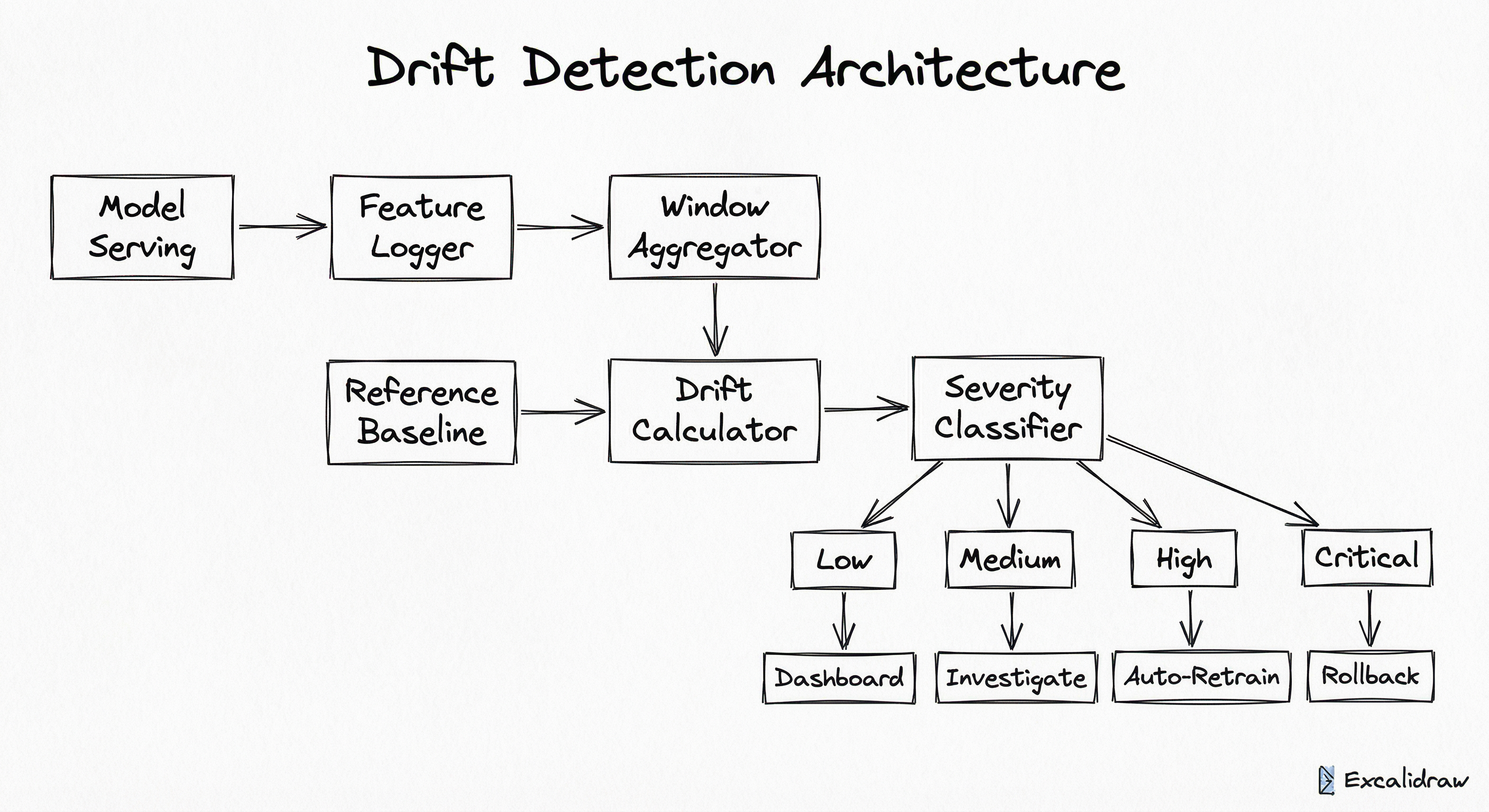
A directed flow showing: Model Serving feeds into Feature Logger, which feeds into Window Aggregator. The Window Aggregator and Reference Baseline both feed into the Drift Calculator. The Drift Calculator feeds into a Severity Classifier, which routes to four outputs based on severity: Dashboard Log (low), Alert Investigate (medium), Auto-Retrain Trigger (high), and Model Rollback (critical).
How to Implement
Implementation Approaches
There are three common approaches to implementing drift detection, each with different trade-offs in complexity, cost, and capability:
Approach 1: Library-based (Evidently, NannyML, Alibi Detect). You integrate a drift detection library into your monitoring pipeline, typically as a scheduled job (Airflow DAG, cron, or Kubernetes CronJob) that runs against logged prediction data. This gives you full control and customizability at the cost of building the orchestration yourself. A team of 2-3 ML engineers at an Indian startup can set this up in 1-2 sprints.
Approach 2: Platform-native (SageMaker Model Monitor, Vertex AI Model Monitoring). Cloud ML platforms offer built-in drift detection as a managed service. You configure monitoring when deploying the model, and the platform handles data collection, statistical testing, and alerting. Less customizable but zero operational overhead. Cost starts at roughly $50/month (~INR 4,200/month) per monitored endpoint on AWS.
Approach 3: Full observability platform (WhyLabs, Arize, Fiddler). Dedicated ML observability platforms that provide drift detection alongside model performance tracking, explainability, and debugging tools. Best for organizations running 10+ models in production that need a unified monitoring dashboard. Pricing typically starts at $500-2,000/month (~INR 42,000-1.68 lakh/month) depending on data volume.
For most teams in the Indian ML ecosystem -- whether at a Bengaluru startup or a large enterprise -- Approach 1 with Evidently AI is the sweet spot: open-source, well-documented, supports all major drift tests, and integrates cleanly with existing monitoring infrastructure (Grafana, Prometheus, Airflow).
import pandas as pd
from evidently.report import Report
from evidently.metric_preset import DataDriftPreset
from evidently.metrics import DataDriftTable

# Load reference (training) and current (production) data
reference_data = pd.read_csv("reference_data.csv")
current_data = pd.read_csv("production_batch_2026_02.csv")

# Create a drift report with all features
report = Report(metrics=[
    DataDriftPreset(),       # Overall drift summary
    DataDriftTable(),        # Per-feature drift details
])

report.run(
    reference_data=reference_data,
    current_data=current_data,
)

# Extract results programmatically
result = report.as_dict()
drift_detected = result["metrics"][0]["result"]["dataset_drift"]
drift_share = result["metrics"][0]["result"]["drift_share"]
print(f"Dataset drift detected: {drift_detected}")
print(f"Share of drifted features: {drift_share:.2%}")

# Save HTML report for visual inspection
report.save_html("drift_report.html")
This example uses Evidently AI's DataDriftPreset to run statistical tests (KS for numerical, chi-squared for categorical) across all features simultaneously. The drift_share metric tells you what percentage of features have drifted -- a value above 0.5 (50%) typically indicates serious distribution shift. The HTML report provides interactive visualizations of per-feature distributions, making it easy to identify which features are the primary culprits.
import numpy as np
from scipy import stats
from typing import Tuple

def ks_drift_test(reference: np.ndarray, current: np.ndarray,
                  alpha: float = 0.05) -> Tuple[float, float, bool]:
    """Run KS test for data drift on a single numerical feature."""
    statistic, p_value = stats.ks_2samp(reference, current)
    drift_detected = p_value < alpha
    return statistic, p_value, drift_detected

def compute_psi(reference: np.ndarray, current: np.ndarray,
                n_bins: int = 10, eps: float = 1e-4) -> float:
    """Compute Population Stability Index between two distributions."""
    # Create bins from reference distribution
    breakpoints = np.quantile(reference, np.linspace(0, 1, n_bins + 1))
    breakpoints[0] = -np.inf
    breakpoints[-1] = np.inf

    # Compute bin proportions
    ref_counts = np.histogram(reference, bins=breakpoints)[0]
    cur_counts = np.histogram(current, bins=breakpoints)[0]

    ref_proportions = ref_counts / len(reference) + eps
    cur_proportions = cur_counts / len(current) + eps

    # PSI formula
    psi = np.sum(
        (cur_proportions - ref_proportions) *
        np.log(cur_proportions / ref_proportions)
    )
    return psi

def classify_psi(psi_value: float) -> str:
    """Classify PSI into severity buckets."""
    if psi_value < 0.1:
        return "no_drift"
    elif psi_value < 0.25:
        return "moderate_drift"
    else:
        return "significant_drift"

# Example usage
reference = np.random.normal(loc=100, scale=15, size=10000)
current = np.random.normal(loc=105, scale=18, size=5000)  # Shifted!

ks_stat, p_val, drifted = ks_drift_test(reference, current)
print(f"KS Statistic: {ks_stat:.4f}, p-value: {p_val:.6f}, Drift: {drifted}")

psi = compute_psi(reference, current)
print(f"PSI: {psi:.4f}, Severity: {classify_psi(psi)}")
This implementation shows drift detection from first principles. The KS test gives you a binary drift/no-drift signal based on the p-value threshold (alpha). PSI gives you a continuous severity score, which is more useful operationally because it tells you how much drift there is, not just whether drift exists. The PSI thresholds (0.1 and 0.25) are industry standards originating from credit risk modeling and work well as defaults for most ML applications.
import nannyml as nml
import pandas as pd

# reference_df has features + predictions + actual targets
# analysis_df has features + predictions (no targets yet!)
reference_df = pd.read_csv("reference_with_labels.csv")
analysis_df = pd.read_csv("production_no_labels.csv")

# Estimate model performance WITHOUT ground truth
estimator = nml.CBPE(
    y_pred_proba="predicted_probability",
    y_pred="predicted_class",
    y_true="actual_class",
    problem_type="classification_binary",
    metrics=["roc_auc", "f1"],
    chunk_size=5000,  # Analysis window size
)
estimator.fit(reference_df)
results = estimator.estimate(analysis_df)

# Check for performance drift
fig = results.plot()
fig.show()

# Univariate feature drift detection
univariate_calculator = nml.UnivariateDriftCalculator(
    column_names=["feature_1", "feature_2", "feature_3"],
    continuous_methods=["kolmogorov_smirnov", "wasserstein"],
    categorical_methods=["chi2", "jensen_shannon"],
    chunk_size=5000,
)
univariate_calculator.fit(reference_df)
drift_results = univariate_calculator.calculate(analysis_df)
print(drift_results.filter(period="analysis").to_df())
NannyML's standout feature is Confidence-Based Performance Estimation (CBPE), which estimates how well your model is performing without needing ground truth labels. This is critical for use cases where labels arrive with a long delay -- loan defaults (6-12 months), customer churn (quarters), or medical diagnoses. CBPE uses the model's own prediction confidence distribution to estimate metrics like AUC and F1, giving you an early signal of degradation weeks before you have actual labels.
import numpy as np
from alibi_detect.cd import MMDDrift
from alibi_detect.cd.pytorch import preprocess_drift
import torch
import torch.nn as nn

# Define a simple feature extractor for high-dimensional data
encoder = nn.Sequential(
    nn.Linear(100, 64),
    nn.ReLU(),
    nn.Linear(64, 32),
)

# Configure the MMD drift detector with a learned kernel
preprocess_fn = preprocess_drift(
    model=encoder,
    batch_size=512,
)

reference_data = np.random.randn(5000, 100).astype(np.float32)

detector = MMDDrift(
    x_ref=reference_data,
    backend="pytorch",
    p_val=0.05,
    preprocess_fn=preprocess_fn,
    n_permutations=500,
)

# Test for drift in new production data
production_data = np.random.randn(2000, 100).astype(np.float32) + 0.3
preds = detector.predict(production_data, return_p_val=True, return_distance=True)

print(f"Drift detected: {preds['data']['is_drift']}")
print(f"p-value: {preds['data']['p_val']:.4f}")
print(f"MMD distance: {preds['data']['distance']:.4f}")
Alibi Detect's MMD test detects multivariate drift that univariate tests (KS, PSI) would miss. By using a learned kernel (the neural network encoder), it can detect subtle shifts in the joint feature distribution even in high-dimensional spaces. This is particularly powerful for image and NLP models where individual pixel or token distributions may not shift, but the overall data manifold does. The trade-off is computational cost: MMD with permutation testing is significantly more expensive than univariate tests.
from airflow import DAG
from airflow.operators.python import PythonOperator
from datetime import datetime, timedelta
import pandas as pd
from evidently.report import Report
from evidently.metric_preset import DataDriftPreset
import json
import requests

DRIFT_THRESHOLDS = {
    "low": 0.3,       # 30% of features drifted
    "medium": 0.5,    # 50% of features drifted
    "high": 0.7,      # 70% of features drifted
    "critical": 0.9,  # 90% of features drifted
}

def run_drift_check(**context):
    """Run drift detection on the latest production window."""
    execution_date = context["execution_date"]
    window_start = execution_date - timedelta(hours=6)
    window_end = execution_date

    # Load data (replace with your data source)
    reference = pd.read_parquet("s3://ml-data/reference/baseline.parquet")
    current = pd.read_parquet(
        f"s3://ml-data/predictions/"
        f"dt={window_start.strftime('%Y-%m-%d-%H')}/"
    )

    report = Report(metrics=[DataDriftPreset()])
    report.run(reference_data=reference, current_data=current)
    result = report.as_dict()

    drift_share = result["metrics"][0]["result"]["drift_share"]
    dataset_drift = result["metrics"][0]["result"]["dataset_drift"]

    # Classify severity
    severity = "none"
    for level, threshold in sorted(
        DRIFT_THRESHOLDS.items(),
        key=lambda x: x[1], reverse=True
    ):
        if drift_share >= threshold:
            severity = level
            break
    if severity == "none" and drift_share >= DRIFT_THRESHOLDS["low"]:
        severity = "low"

    context["ti"].xcom_push(key="drift_share", value=drift_share)
    context["ti"].xcom_push(key="severity", value=severity)
    return {"drift_share": drift_share, "severity": severity}

def route_alert(**context):
    """Route alert based on drift severity."""
    severity = context["ti"].xcom_pull(
        task_ids="run_drift_check", key="severity"
    )
    drift_share = context["ti"].xcom_pull(
        task_ids="run_drift_check", key="drift_share"
    )

    if severity in ("high", "critical"):
        # Trigger retraining pipeline
        requests.post(
            "https://airflow.internal/api/v1/dags/retrain_model/dagRuns",
            json={"conf": {"trigger": "drift", "severity": severity}},
            headers={"Authorization": "Bearer <token>"},
        )
        # Alert on-call
        requests.post(
            "https://hooks.slack.com/services/YOUR/WEBHOOK/URL",
            json={"text": (
                f":rotating_light: *DRIFT ALERT [{severity.upper()}]*\n"
                f"Drift share: {drift_share:.1%}\n"
                f"Action: Retraining pipeline triggered automatically."
            )},
        )
    elif severity == "medium":
        requests.post(
            "https://hooks.slack.com/services/YOUR/WEBHOOK/URL",
            json={"text": (
                f":warning: *Drift Warning [{severity.upper()}]*\n"
                f"Drift share: {drift_share:.1%}\n"
                f"Action: Please investigate feature distributions."
            )},
        )

dag = DAG(
    "drift_monitoring",
    schedule_interval="0 */6 * * *",  # Every 6 hours
    start_date=datetime(2026, 1, 1),
    catchup=False,
    default_args={"retries": 2, "retry_delay": timedelta(minutes=5)},
)

check_task = PythonOperator(
    task_id="run_drift_check",
    python_callable=run_drift_check,
    dag=dag,
)

alert_task = PythonOperator(
    task_id="route_alert",
    python_callable=route_alert,
    dag=dag,
)

check_task >> alert_task
This is a production-grade Airflow DAG that runs drift detection every 6 hours. It demonstrates the full pipeline: load reference and production data, run statistical tests via Evidently, classify drift severity using configurable thresholds, and route alerts accordingly. High/critical drift automatically triggers a retraining pipeline, while medium drift sends a Slack warning for human investigation. The 6-hour window balances detection speed against statistical reliability -- adjust based on your traffic volume.
# drift-detection-config.yaml
# Production drift monitoring configuration

model:
  name: fraud-detection-v3
  version: "3.2.1"
  endpoint: https://model-serving.internal/fraud/v3

reference:
  source: s3://ml-baselines/fraud-v3/reference.parquet
  refresh_policy: on_retrain  # Update baseline after each retraining

monitoring:
  window_size: 6h          # Tumbling window duration
  min_samples: 500         # Minimum samples before running tests
  schedule: "0 */6 * * *"  # Cron: every 6 hours

features:
  numerical:
    tests: [ks, wasserstein, psi]
    ks_alpha: 0.05
    psi_warning: 0.1
    psi_critical: 0.25
  categorical:
    tests: [chi2, jensen_shannon]
    chi2_alpha: 0.05
    jsd_warning: 0.1
    jsd_critical: 0.2
  ignore:
    - request_id
    - timestamp
    - user_id
  high_priority:  # Features with elevated alert sensitivity
    - transaction_amount
    - merchant_category
    - device_fingerprint

severity:
  levels:
    low:
      drift_share: 0.2       # 20% of features drifted
      action: log_only
    medium:
      drift_share: 0.4
      action: slack_alert
    high:
      drift_share: 0.6
      action: slack_alert + trigger_investigation
    critical:
      drift_share: 0.8
      action: trigger_retraining + page_oncall

alerting:
  cooldown: 2h               # Min time between alerts for same model
  channels:
    slack: "#ml-alerts"
    pagerduty: ml-oncall-rotation
  suppression_windows:        # Known events where drift is expected
    - name: diwali_sale
      start: "2026-10-20"
      end: "2026-11-05"
    - name: ipl_season
      start: "2026-03-22"
      end: "2026-05-28"
Common Implementation Mistakes
- ●
Using a single test for all feature types: The KS test is designed for continuous numerical features. Applying it to categorical features (city names, device types) produces meaningless results. Use chi-squared or Jensen-Shannon divergence for categorical features, KS or Wasserstein for numerical ones. Evidently and NannyML handle this automatically, but custom implementations often get it wrong.
- ●
Setting thresholds too aggressively on high-volume data: With large sample sizes (millions of predictions/day), even trivially small distribution shifts become statistically significant. A p-value of 0.001 on a KS test with 10 million samples might represent a shift so small it has zero impact on model performance. Always complement statistical significance with practical significance -- use effect size metrics (PSI, Wasserstein) alongside p-values.
- ●
Monitoring all features with equal weight: Not all features matter equally for model performance. A drift in a feature with near-zero importance (feature_importance < 0.01) is not worth alerting on. Weight your drift signals by feature importance, or focus monitoring on the top 10-20 features that drive 80% of the model's predictive power.
- ●
Forgetting to update the reference baseline after retraining: After you retrain a model on new data, the old reference baseline becomes stale. If you do not update it, your drift detector will compare production data against an outdated baseline and produce confusing results -- potentially suppressing real drift or flagging expected changes as anomalies.
- ●
Running drift checks on every prediction (over-monitoring): Running a KS test after every single prediction is both computationally expensive and statistically unsound (tiny sample sizes give wildly unstable results). Batch your checks into windows of at least a few hundred observations. For low-traffic models, daily or weekly windows are appropriate.
- ●
Ignoring seasonality and known events: Drift detection systems that do not account for expected distribution shifts (holiday shopping seasons, IPL cricket season, Diwali sales, month-end salary cycles) will generate a flood of false positives. Implement suppression rules or use seasonal reference baselines that match the current calendar period.
When Should You Use This?
Use When
Your model serves predictions in production and you need early warning of performance degradation before ground truth labels are available
Ground truth labels arrive with significant delay (days to months) -- common in credit scoring, churn prediction, medical diagnostics, and ad conversion models
Your input data is subject to real-world distribution changes: seasonal patterns, user behavior shifts, regulatory changes, or upstream data pipeline modifications
You operate in a regulated industry (banking, insurance, healthcare) where model performance documentation and drift monitoring is a compliance requirement -- RBI guidelines in India increasingly expect this for credit models
You run multiple models in production and need automated, scalable monitoring rather than manual periodic reviews
Your business is sensitive to model degradation -- e.g., a 1% drop in fraud detection recall at Razorpay could mean lakhs in losses per day
You are implementing CI/CD for ML models and need drift metrics as deployment gates (block deployment if incoming data has drifted too far from training data)
Avoid When
Your model is retrained on fresh data before every inference batch (no gap between training and serving distributions) -- common in some recommendation systems
You have immediate access to ground truth labels and can directly monitor model performance in real time -- drift detection becomes redundant if you can just watch accuracy/AUC directly
Your model operates in a truly stationary environment where the data-generating process does not change (rare in practice, but some physics-based models qualify)
You have fewer than 100 predictions per monitoring window -- the sample sizes are too small for statistical tests to be reliable, and you will get noisy, unreliable results
The cost of false drift alarms exceeds the cost of occasional model degradation -- for low-stakes models where retraining is cheap and frequent, the monitoring overhead may not be justified
You are still in the experimentation phase and the model is not yet in production -- drift detection is a production concern, not a development-time concern
Key Tradeoffs
Sensitivity vs. False Alarm Rate
The fundamental tradeoff in drift detection mirrors the classic precision-recall tension. Lower p-value thresholds and smaller PSI warning levels catch more real drift (higher sensitivity) but also trigger more false alarms. Higher thresholds miss some real drift but reduce alert fatigue.
In practice, alert fatigue is the bigger danger. A drift detection system that cries wolf every day will be ignored within a week, and then the one real drift event that matters will go unnoticed. Start with conservative thresholds (PSI > 0.25 for warning, > 0.5 for critical) and tighten only if you find you are missing real drift events.
Univariate vs. Multivariate Testing
| Dimension | Univariate (KS, PSI per feature) | Multivariate (MMD, domain classifier) |
|---|---|---|
| Interpretability | High -- you know exactly which feature drifted | Low -- "the joint distribution shifted" is hard to act on |
| Computational cost | Low -- O(n) per feature | High -- O(n^2) for kernel methods |
| Detection power | Misses correlated shifts | Catches joint distribution changes |
| False positive rate | Higher (multiple testing problem) | Lower per test, but harder to threshold |
| Recommended use | Primary production monitoring | Periodic deep audits, complex data |
Most production systems run univariate tests as the first line of defense (fast, interpretable, actionable) and reserve multivariate tests for periodic deep dives or when univariate results are inconclusive.
Detection Speed vs. Statistical Reliability
Smaller analysis windows (1 hour) detect drift faster but with higher variance in test statistics. Larger windows (24 hours) produce more reliable results but delay detection. The right window size depends on your traffic volume and acceptable detection latency.
| Daily predictions | Recommended window | Detection latency |
|---|---|---|
| < 1,000 | 24 hours | ~1 day |
| 1,000 - 50,000 | 6 hours | ~6 hours |
| 50,000 - 1M | 1 hour | ~1 hour |
| > 1M | 15-30 minutes | ~30 minutes |
Cost Note: Running drift detection on every 6-hour window for a model with 50 features costs approximately $30-50/month (~INR 2,500-4,200/month) on AWS Lambda/Fargate. On a dedicated EC2 instance, it is essentially free since the compute is minimal.
Alternatives & Comparisons
Data validation catches hard errors -- missing columns, type mismatches, null spikes, out-of-range values -- while drift detection catches soft shifts in valid data. They are complementary: data validation is your first line of defense (fast, deterministic), drift detection is your second (statistical, probabilistic). Run data validation before drift detection; many apparent drift signals are actually upstream data quality bugs.
Direct performance monitoring (tracking accuracy, F1, AUC on labeled data) is the gold standard for detecting model degradation. But it requires ground truth labels, which often arrive late. Drift detection provides a leading indicator when labels are delayed. In a complete monitoring stack, you want both: drift detection for early warning, performance monitoring for confirmation.
Simple threshold alerting (e.g., alert if prediction mean drops below X) catches obvious anomalies but misses subtle distributional shifts that statistical tests detect. Drift detection is more principled and catches shifts that fixed thresholds miss. However, threshold alerting is simpler to implement and easier to reason about -- start there if you are building monitoring from scratch.
Pros, Cons & Tradeoffs
Advantages
Early warning without labels: Detects potential model degradation weeks or months before ground truth labels are available, giving you a critical head start on remediation -- especially valuable for credit models, churn prediction, and healthcare applications where label delay is inherent
Feature-level attribution: Univariate drift tests pinpoint exactly which features are drifting, making root cause analysis actionable. When your Slack alert says 'transaction_amount PSI = 0.38', your ML engineer knows exactly where to look
Statistical rigor: Well-established mathematical foundations (KS test, Wasserstein distance, MMD) provide principled detection with quantifiable confidence levels, unlike ad-hoc threshold monitoring
Automation-friendly: Drift scores integrate naturally into CI/CD pipelines as deployment gates and into orchestration systems as retraining triggers, enabling truly automated ML operations
Regulatory compliance: Increasingly required by financial regulators (RBI in India, OCC in the US, PRA in the UK) for credit scoring and risk models. Having drift monitoring in place makes audits significantly easier
Cost-effective prevention: Catching drift early prevents costly silent failures. Uber's D3 system saved them tens of millions of dollars by detecting data quality issues before they impacted downstream ML models
Disadvantages
Not all drift is harmful: Distribution shifts do not always cause model performance degradation. Over-reacting to benign drift wastes engineering time and compute resources on unnecessary retraining. You need to learn which drift signals to act on, which takes operational experience
Multiple testing problem: When monitoring 50+ features, some will appear to drift by chance alone (at alpha=0.05, you expect ~2.5 false positives out of 50 tests). Bonferroni or FDR correction helps but reduces power. This is a genuine statistical challenge with no perfect solution
Concept drift is hard to detect directly: Data drift (input distribution shift) is relatively easy to detect. Concept drift (changed input-output relationship) is much harder because it requires labels or proxy metrics. Most tools primarily detect data drift, not concept drift
Sample size sensitivity: Statistical tests behave differently at different sample sizes. With very large samples, trivial differences become 'significant'. With very small samples, real drift goes undetected. Calibrating thresholds requires ongoing attention
Operational overhead: Setting up and maintaining drift monitoring adds complexity to your ML platform. Reference baselines need updating, thresholds need tuning, suppression rules need maintaining, and false alarms need triaging. For a single low-stakes model, this overhead may not be justified
Seasonal blindness: Standard drift detection compares against a fixed reference and cannot distinguish expected seasonal variation from genuine harmful drift. Without seasonality-aware baselines, you will get false alarms during every holiday season, IPL match day, or month-end salary cycle
Failure Modes & Debugging
Alert fatigue from false positives
Cause
Thresholds set too aggressively, no correction for multiple testing, or failure to account for expected seasonal variation. Common when a team first deploys drift detection and uses textbook p-value thresholds (0.05) without considering their data volume or feature count.
Symptoms
The #ml-alerts Slack channel is flooded with drift warnings daily. Engineers start ignoring alerts. When a real, harmful drift event occurs, nobody notices because the signal is lost in the noise. The drift monitoring system becomes shelfware within weeks.
Mitigation
Start with conservative thresholds (PSI > 0.25 for warning). Apply Benjamini-Hochberg FDR correction for multiple testing. Implement suppression windows for known events (Diwali, IPL). Weight drift alerts by feature importance. Track the false positive rate and adjust thresholds quarterly.
Missed concept drift (detecting inputs but not relationships)
Cause
Over-reliance on data drift (covariate shift) detection while ignoring concept drift. The input features look stable, but the relationship between features and the target has changed. Most drift detection tools primarily monitor inputs, not the input-output mapping.
Symptoms
Model performance degrades on actual labels (when they finally arrive), but the drift monitoring dashboard shows green across all features. The team loses trust in the monitoring system: 'We had drift detection and it did not catch the problem.'
Mitigation
Complement data drift monitoring with: (1) prediction drift monitoring (track the output distribution), (2) performance estimation without labels (NannyML's CBPE), (3) delayed label monitoring when ground truth becomes available. A multi-signal approach catches what any single test misses.
Stale reference baseline
Cause
The reference distribution is not updated after model retraining. The model was retrained on recent data (which has naturally shifted), but drift detection still compares production data against the original training distribution from months ago.
Symptoms
Persistent low-grade drift alerts that never resolve, even though the model is performing well. OR drift detection shows 'no drift' because the reference is so old that its tolerance has become meaninglessly wide. Both outcomes erode trust in the system.
Mitigation
Automate reference baseline updates as part of the retraining pipeline. After each retraining, recompute the reference profile from the new training data and deploy it alongside the new model. Version-tag baselines so you can trace which reference corresponds to which model version.
Statistical power failure on low-traffic models
Cause
Running drift tests on analysis windows with too few samples. A KS test with 50 observations has very low power -- it will miss real drift because the sample is too small to detect it reliably.
Symptoms
Drift detection consistently reports 'no drift' even when visual inspection of distributions clearly shows a shift. The p-values are always high because the sample is too small to achieve significance. The monitoring system provides false confidence.
Mitigation
Enforce minimum sample size requirements before running tests (typically 200-500 observations). For low-traffic models, use wider analysis windows (daily or weekly instead of hourly). Consider using effect-size metrics (PSI, Wasserstein) that are more robust at small sample sizes than hypothesis tests.
Upstream data pipeline corruption misdiagnosed as drift
Cause
A data pipeline bug (e.g., a feature column filled with nulls, a unit conversion error, a schema change) causes a sudden distribution shift. The drift detector correctly identifies the shift but labels it as 'data drift' when it is actually a data quality issue.
Symptoms
Sudden, sharp drift signal across multiple features simultaneously. The drift is not a gradual shift but a step-change. Automated retraining triggers fire, but retraining on corrupted data makes the problem worse.
Mitigation
Run data validation checks (schema validation, null rate monitoring, value range checks) upstream of drift detection. If data validation fails, skip drift detection entirely and route to the data engineering team. The order matters: validate first, then detect drift.
Multivariate drift invisible to univariate tests
Cause
The marginal distribution of each feature remains stable, but the joint distribution (correlations between features) has shifted. For example, age and income individually look the same, but the age-income relationship has changed.
Symptoms
All per-feature drift tests pass, but model performance degrades. The drift monitoring dashboard is entirely green while downstream business metrics are declining. This is particularly dangerous because it creates a false sense of security.
Mitigation
Periodically run multivariate drift tests (MMD, domain classifier approach) in addition to per-feature tests. Monitor feature correlation matrices over time. Track prediction distribution drift as a complementary signal -- even if inputs look individually stable, shifted correlations often show up in the prediction distribution.
Placement in an ML System
Where Drift Detection Fits in the ML System
Drift detection sits in the monitoring layer, operating on data that flows out of the serving layer. It is a post-deployment concern -- it activates only after a model is live and receiving real traffic.
The placement is critical: drift detection must be downstream of model serving (it needs predictions and features to analyze) but upstream of alerting and retraining (it feeds signals that trigger those systems).
In a typical Kubernetes-based ML platform (common at companies like Swiggy, Zomato, and PhonePe), drift detection runs as a separate service or CronJob, not as part of the serving pod. This decoupling ensures that drift detection failures do not impact serving latency or availability.
The data flow is: Model Server -> Feature Logger (async, via Kafka or similar) -> Drift Detection Service -> Alert System / Retraining Pipeline. The Feature Logger is the integration point: it captures the same features that the model consumes, plus the model's predictions, and routes them to storage for analysis.
Key Insight: Drift detection is not an add-on; it is a core component of any production ML system. Without it, you are flying blind -- making predictions with no way to know when those predictions stop being trustworthy.
Pipeline Stage
Monitoring / Post-Deployment
Upstream
- model-serving
- feature-store
- data-validation
Downstream
- alerting
- metrics-collector
- model-training
Scaling Bottlenecks
The primary bottleneck is data volume at the feature logger. A model serving 10 million predictions/day with 50 features generates ~500 million feature values per day that need to be logged, stored, and aggregated. At 8 bytes per float64 value, that is ~4 GB/day of raw feature data before any overhead.
The statistical tests themselves are cheap -- a KS test over 100K observations runs in milliseconds. The expense is in the data pipeline: collecting, storing, and windowing the feature logs.
At Uber scale (millions of models, billions of predictions), they solved this with streaming aggregation via Apache Flink, computing approximate statistics (t-digest for quantiles, approximate histograms) in-stream rather than storing raw feature values. This reduces storage by 100x while preserving enough statistical fidelity for drift detection.
For most Indian ML teams, the bottleneck is more prosaic: the cost of storing feature logs in S3 or BigQuery. Budget approximately $50-100/month (~INR 4,200-8,400/month) per monitored model for storage and compute at moderate traffic (100K predictions/day).
Production Case Studies
Uber built D3 (Dataset Drift Detector), an automated system that monitors column-level data quality across petabytes of data. D3 automatically determines important columns based on offline usage patterns and applies monitors without manual configuration. The system uses historical column statistics (computed over 90-day windows) as reference baselines and runs daily scheduled jobs to detect column-level drift.
D3 reduced the median time to detect issues in critical datasets by 5x and saved Uber tens of millions of dollars in incremental revenue by catching data quality issues before they impacted downstream ML models. The system scaled to thousands of datasets with single-click onboarding.
Netflix built an ML observability platform that tracks prediction quality, feature drift, and business metrics across their model fleet. The platform integrates with Metaflow (their open-source ML infrastructure framework) and enables data scientists to schedule monitoring notebooks that compare live feature distributions against training baselines. Canary deployment strategies gradually roll out new models to small user segments, with drift detection serving as one of the automated rollback criteria.
The observability platform provides real-time transparency into ML model behavior across payments, recommendations, and content delivery. Automated canary monitoring catches model regressions within minutes of deployment, reducing the blast radius of bad model updates.
Uber's Hue observability stack (part of the Michelangelo ML platform) provides continuous monitoring of ML models in production. Hue tracks operational metrics (availability, latency, throughput) alongside prediction-level indicators (score distributions, calibration, entropy). Feature health checks run in real time, detecting drift via statistical tests and verifying online-offline feature parity. Hue supports slicing by region, caller, or custom dimensions for precise debugging.
Hue detects prediction drift, verifies online-offline parity, and surfaces anomalies within minutes. The system operates at Uber scale via a streamlined Apache Flink job deployed through Flink-as-a-Service and backed by Apache Pinot for real-time analytics.
Indian fintech companies like Razorpay, processing millions of transactions daily, face continuous concept drift in fraud detection as attackers evolve their tactics. The UPI ecosystem in India saw transaction volumes grow from 2.3 billion/month in 2020 to over 14 billion/month in 2025, fundamentally shifting the distribution of transaction amounts, merchant categories, and user behavior patterns. Fraud detection models trained on pre-UPI-surge data face severe data drift and concept drift simultaneously.
Continuous drift monitoring on transaction features (amount distribution, merchant category mix, device fingerprints, geographic patterns) enables fintech companies to trigger model retraining within hours of detecting significant shifts, keeping fraud detection recall above 95% even as payment patterns evolve rapidly.
Tooling & Ecosystem
Open-source Python library for ML and LLM observability. Provides 100+ built-in evaluation metrics including 20+ statistical drift detection tests (KS, PSI, Wasserstein, Jensen-Shannon, chi-squared). Generates interactive HTML reports and integrates with Grafana, MLflow, and Airflow. Supports tabular data, text data, and both predictive and generative AI monitoring. The most widely adopted open-source drift detection tool.
Open-source library specializing in performance estimation without ground truth labels using CBPE (Confidence-Based Performance Estimation). Also provides univariate drift detection (KS, Wasserstein, Jensen-Shannon, L-Infinity, chi-squared) and multivariate drift detection via PCA-based reconstruction error. Particularly valuable when labels arrive with long delays. Available under Apache 2.0 license with a cloud version for managed monitoring.
Source-available Python library focused on outlier, adversarial, and drift detection. Supports both online (streaming) and offline (batch) detection for tabular data, text, images, and time series. Implements advanced methods including MMD with learned kernels, LSDD (Least-Squares Density Difference), and classifier-based drift detection. Supports both TensorFlow and PyTorch backends. Integrated with Seldon Core for serving-time monitoring.
Managed service for monitoring ML models deployed on SageMaker. Automatically detects data quality drift, model quality drift, bias drift, and feature attribution drift. Supports custom monitoring rules and thresholds. Integrates with CloudWatch for alerting and SageMaker Studio for visualization. Pricing is based on processing jobs (~$0.05/GB processed).
Managed monitoring for models deployed on Vertex AI. Uses TensorFlow Data Validation (TFDV) under the hood to compute L-infinity distance and Jensen-Shannon divergence for feature skew and drift. Logs prediction requests to BigQuery and runs scheduled monitoring jobs. Supports email and Slack alerting when drift exceeds configured thresholds.
Open-source data logging library that computes privacy-preserving statistical profiles (histograms, quantile sketches, cardinality estimates) of datasets. Profiles can be compared across time periods to detect drift without storing raw data. The WhyLabs AI Control Center (now open source) provides a monitoring dashboard. Particularly good for organizations with strict data privacy requirements.
While primarily a data validation tool (schema checks, value ranges, null rates), Great Expectations complements drift detection by catching hard data quality failures upstream. Its expectation suite pattern makes it easy to define data quality contracts that serve as a first line of defense before statistical drift tests run.
Research & References
Rabanser, Gunnemann & Lipton (2019)NeurIPS 2019
A landmark empirical study comparing methods for detecting dataset shift. Found that two-sample tests with pretrained classifiers for dimensionality reduction perform best. Introduced the framework of 'failing loudly' -- the principle that ML systems should actively detect when their inputs have shifted rather than silently degrading.
Lu, Liu, Dong, Gu, Gama & Zhang (2019)IEEE Transactions on Knowledge and Data Engineering
Comprehensive survey establishing a framework for learning under concept drift with three components: detection, understanding, and adaptation. Categorizes drift types (sudden, gradual, incremental, recurring) and reviews detection methods from statistical tests to adaptive learning algorithms.
Gama, Zliobait\u0117, Bifet, Pechenizkiy & Bouchachia (2014)ACM Computing Surveys
Foundational survey by Joao Gama and colleagues characterizing adaptive learning processes and categorizing strategies for handling concept drift in data streams. Introduced the influential taxonomy of drift handling mechanisms: detectors, adaptive learners, and ensemble methods.
Various (2024)arXiv preprint
Introduces the Prediction Uncertainty Index (PU-index) as a drift detection signal derived from classifier prediction uncertainty. Demonstrates that the PU-index can detect drift even when error rates remain stable, providing an earlier warning than traditional performance-based detection.
Various (2024)arXiv preprint
Cross-field review distinguishing between domain shift (data source changes with unchanged model performance) and concept drift (time-varying phenomena causing model obsolescence). Covers detection, adaptation, and mitigation strategies across computer vision, NLP, and tabular data domains.
Gama et al. (2024)Frontiers in Artificial Intelligence
A 2024 survey focused specifically on drift detection and monitoring in evolving environments. Part A covers detection methods (ADWIN, DDM, EDDM, Page-Hinkley) and their comparative performance. Found that ADWIN and Page-Hinkley consistently demonstrate superior detection performance across benchmark datasets.
Interview & Evaluation Perspective
Common Interview Questions
- ●
What is the difference between data drift, concept drift, and prediction drift? Give a real-world example of each.
- ●
How would you design a drift detection system for a model that receives 1 million predictions per day across 100 features?
- ●
The KS test says a feature has drifted (p < 0.05) but model performance has not changed. What do you do?
- ●
How do you handle drift detection when ground truth labels are delayed by 6 months?
- ●
You have 100 features. How do you deal with the multiple testing problem in drift detection?
- ●
How would you set drift thresholds for a fraud detection model at an Indian fintech company?
- ●
Describe how you would implement automated retraining triggered by drift detection. What safety checks would you put in place?
- ●
What are the limitations of drift detection? When does it fail to catch model degradation?
Key Points to Mention
- ●
Clearly distinguish the three types of drift: data drift (P(X) changes), concept drift (P(Y|X) changes), prediction drift (P(Y_hat) changes). Each requires different detection approaches and has different implications.
- ●
Statistical significance is not the same as practical significance. At large sample sizes, trivially small shifts become statistically significant. Always pair p-value-based tests with effect-size metrics (PSI, Wasserstein distance).
- ●
Drift detection is a leading indicator -- it tells you something has changed before you have labels to confirm performance degradation. This temporal advantage is the primary value proposition.
- ●
Not all drift is harmful. The correct response to a drift signal is investigation, not automatic retraining. Build severity tiers and respond proportionally.
- ●
The multiple testing problem is real: testing 50 features at alpha=0.05 yields ~2.5 false positives by chance. Apply Bonferroni or Benjamini-Hochberg correction, or aggregate into a 'drift share' metric.
- ●
Reference baselines must be updated after each retraining cycle. Stale baselines produce meaningless drift signals.
Pitfalls to Avoid
- ●
Claiming drift detection can replace performance monitoring -- it cannot. Drift detection is a complement to, not a substitute for, tracking actual model accuracy when labels are available.
- ●
Ignoring the multiple testing problem when monitoring many features simultaneously. Reporting 3 out of 50 features as 'drifted' at p < 0.05 is not necessarily meaningful.
- ●
Suggesting that all drift requires immediate retraining. Many drift events are benign, seasonal, or self-correcting. Knee-jerk retraining can make things worse if the training data window includes the drifted period.
- ●
Treating drift detection as a one-time setup. Thresholds need ongoing tuning, reference baselines need updating, and suppression rules need maintenance. It is an operational commitment, not a deploy-and-forget solution.
- ●
Not discussing the latency between detection and action. Detecting drift in 1 hour is useless if retraining takes 2 weeks. The entire response pipeline matters.
Senior-Level Expectation
A senior/staff-level candidate should discuss drift detection as part of a broader ML observability strategy, not in isolation. They should articulate the full detection-to-resolution pipeline: (1) feature logging architecture (async, not on the serving path), (2) windowing strategy with justification for window sizes, (3) statistical test selection based on feature types and data volumes, (4) multiple testing correction, (5) severity classification with business-context-aware thresholds, (6) suppression rules for known events, (7) automated vs. human-in-the-loop response policies, (8) reference baseline lifecycle management, and (9) the relationship between drift detection and the retraining pipeline (including safety checks to prevent retraining on corrupted data). They should also discuss cost optimization -- monitoring at Uber scale vs. a startup with 3 models is fundamentally different, and the architecture should reflect that. Bonus points for discussing how concept drift detection differs from data drift detection and the limitations of current tools in catching concept drift without labels.
Summary
Recap
Drift detection is the practice of continuously monitoring whether the statistical properties of production data, model predictions, and input-output relationships have diverged from what the model was trained on. It addresses the fundamental challenge that ML models degrade silently -- unlike software bugs that crash loudly, a drifting model produces confident but increasingly wrong predictions without any obvious error signal.
The three types of drift -- data drift ( shifts), concept drift ( shifts), and prediction drift ( shifts) -- each require different detection approaches. Data drift is the easiest to detect using statistical two-sample tests (KS test for continuous features, chi-squared for categorical, PSI for severity scoring, Wasserstein distance for shift magnitude). Concept drift is harder because it requires labels or proxy estimation methods like NannyML's CBPE. Prediction drift is a useful complementary signal that can reveal issues even when individual features appear stable.
The production architecture follows a decoupled pattern: async feature logging (never on the serving path), windowed aggregation, statistical testing against a versioned reference baseline, severity classification, and tiered alert routing. The tools ecosystem is mature -- Evidently AI for comprehensive open-source monitoring, NannyML for label-free performance estimation, Alibi Detect for advanced multivariate detection, and managed options from AWS, Google Cloud, and dedicated platforms like WhyLabs for teams that prefer less operational overhead.
The most important lesson in drift detection is restraint: not all drift is harmful, not all alarms warrant action, and not every drift event should trigger retraining. The goal is not to eliminate drift (you cannot -- the world changes) but to detect it early enough and respond proportionally. Build severity tiers, suppress known events, validate before retraining, and update your baselines. Done well, drift detection transforms your ML operations from reactive firefighting into proactive, data-driven model management.