What is the difference between a copula and a correlation matrix?

A **correlation matrix** is a specific numerical summary of linear (Pearson) or rank-based (Kendall, Spearman) associations between pairs of variables. It captures a single number per pair -- the strength and direction of their linear relationship. A **copula** is a much richer object: it is the entire joint distribution function of the uniform-transformed variables, capturing the **full dependency structure** including non-linear patterns, asymmetries, and tail behavior. The correlation matrix is a parameter of some copulas (e.g., it fully characterizes the Gaussian copula), but other copulas can capture dependencies that no single correlation number can describe. For example, the Clayton copula has strong **lower tail dependence** (variables tend to be extreme together at the low end) but weak upper tail dependence. No correlation coefficient captures this asymmetry. The Gaussian copula uses the correlation matrix as its sole parameter, which is why it cannot model tail dependence at all. In practice, when people say "copula generator," they often mean the Gaussian copula, where the correlation matrix IS the copula (up to the normal transform). But the copula framework is broader, encompassing Archimedean copulas, vine copulas, and other families that go well beyond linear correlation.

How does a copula generator compare to CTGAN for tabular data?

The comparison depends heavily on your dataset and priorities: **Copula generator wins when**: (1) Training speed matters -- seconds vs. minutes-to-hours for CTGAN. (2) Interpretability is required -- regulators and auditors can inspect the correlation matrix and marginal parameters directly. (3) Your data is primarily numerical with well-characterized pairwise correlations. (4) You need deterministic, reproducible results. (5) You have no GPU available. **CTGAN wins when**: (1) Your data has complex non-linear relationships that pairwise correlations cannot capture. (2) You have many high-cardinality categorical columns -- CTGAN's mode-specific normalization handles these natively. (3) Your data has multimodal continuous distributions that are hard to fit parametrically. (4) You need the synthetic data to preserve downstream ML model performance (CTGAN often achieves higher ML efficacy scores). Recent benchmarks (2024-2025) show that Gaussian copulas rank second overall in total variation distance after Bayesian networks, while CTGAN ranks lower on correlation preservation but higher on capturing complex distributional patterns. A pragmatic approach: **start with the Gaussian copula as your baseline**. If the quality score exceeds 0.85 and downstream ML performance is acceptable, stop there. If not, try CTGAN or consider a hybrid like SDV's `CopulaGANSynthesizer` which uses a GAN for marginals and a copula for correlations.

Can copula generators provide differential privacy guarantees?

Standard copula generators do **not** provide differential privacy (DP) guarantees out of the box. The correlation matrix and marginal parameters are computed directly from the training data and could, in theory, be used to reconstruct or infer individual records -- especially when the training set is small. However, copula generators can be **augmented with DP mechanisms**: 1. **DP correlation matrix**: Add calibrated Gaussian or Laplace noise to each entry of the correlation matrix before using it for sampling. The noise magnitude is calibrated to the sensitivity of the correlation estimator (bounded by $O(1/n)$ for $n$ samples) and the desired privacy budget $\epsilon$. 2. **DP marginal fitting**: Add noise to the sufficient statistics of each marginal distribution (e.g., noisy mean and variance for Gaussian marginals). For empirical CDFs, use the exponential mechanism to select histogram bin counts. 3. **TVineSynth approach**: The recent TVineSynth paper (2025) uses truncation of the vine copula tree structure as a privacy mechanism -- by limiting the depth of the vine, you limit how much information about individual records is encoded in the model. The key challenge is that DP noise on the correlation matrix can destroy the positive semi-definiteness guarantee, requiring additional post-processing (nearest-PSD projection). This noise also degrades the quality of the synthetic data -- the privacy-utility tradeoff. For strong privacy ($\epsilon < 1.0$), expect a 10-25% drop in quality scores compared to the non-private copula.

What is the role of the probability integral transform (PIT) in copula modeling?

The **probability integral transform** is the mathematical bridge that makes copula modeling work. It is based on a simple but profound result: if $X$ is a continuous random variable with CDF $F_X$, then $U = F_X(X)$ is uniformly distributed on $[0, 1]$. Why is this useful? Because copulas are defined on **uniform marginals** -- they describe the dependency structure between variables that are all uniformly distributed on $[0, 1]$. To apply copula theory to real data (where columns follow arbitrary distributions -- normal, log-normal, gamma, etc.), you first need to transform each column to uniform. The PIT does exactly this: for each column, apply its fitted CDF to transform the data to uniform. Now all columns live in the same $[0, 1]$ space, and you can fit a copula to capture how they move together. The **inverse PIT** reverses the process during generation: given uniform samples from the copula, apply each column's inverse CDF (quantile function) to transform back to the original scale. This ensures that the generated data has the correct marginal distributions while preserving the copula-induced dependency structure. A common pitfall: if your marginal CDF is poorly fitted, the PIT will produce non-uniform results, and the copula estimation will be biased. Always validate uniformity of the PIT-transformed data using histograms or the Kolmogorov-Smirnov test.

How do vine copulas differ from the standard Gaussian copula?

The **Gaussian copula** models all dependencies through a single correlation matrix in the normal-transformed space. It has one big limitation: it can only capture **symmetric, tail-independent** dependencies. The correlation matrix tells you the average association between pairs of variables, but it cannot distinguish whether two variables are more correlated during extreme events (tail dependence) or whether their relationship is asymmetric (e.g., correlated during downturns but not during rallies). **Vine copulas** address these limitations by decomposing the $d$-dimensional dependency structure into a sequence of **bivariate copulas** arranged in a tree (vine) structure. Each bivariate copula can be chosen from any family: - **Clayton**: Strong lower tail dependence (good for modeling simultaneous crashes) - **Gumbel**: Strong upper tail dependence - **Student-t**: Symmetric tail dependence (both extremes) - **Frank**: Symmetric, no tail dependence (like Gaussian but with different shape) - **Joe**: Upper tail dependence, different from Gumbel The vine structure determines which pairs of variables are modeled directly and which are modeled conditionally. A **C-vine** places one "central" variable that connects to all others. A **D-vine** arranges variables in a sequence. An **R-vine** (regular vine) allows arbitrary structures. The tradeoff: vine copulas are more expressive but also more complex. Fitting a Gaussian copula requires estimating $\binom{d}{2}$ correlations. Fitting a vine copula requires selecting the tree structure AND choosing a copula family AND estimating parameters for each of $\binom{d}{2}$ bivariate copulas. For 50 columns, that is 1,225 bivariate copulas to fit and select.

What was the role of the Gaussian copula in the 2008 financial crisis?

The Gaussian copula became infamous in the 2008 financial crisis through its use in pricing **Collateralized Debt Obligations (CDOs)**. David X. Li's 2000 paper proposed using the Gaussian copula to model the joint default behavior of mortgages bundled into CDO tranches. The model worked as follows: each mortgage's default time was modeled as a marginal distribution, and the Gaussian copula captured the **correlation** between defaults. The key parameter was the **default correlation** -- how likely it was that if one mortgage defaulted, others would too. The critical flaw was the Gaussian copula's **zero tail dependence**. In mathematical terms, $\lim_{u \to 0} \lambda_L = 0$ -- the probability that many mortgages default simultaneously (given that some have defaulted) converges to zero as you look at more extreme events. The model predicted that widespread simultaneous defaults were essentially impossible. When the US housing market crashed in 2007-2008, exactly this "impossible" scenario materialized. Mortgage defaults were highly correlated during the stress event -- a phenomenon the Gaussian copula structurally could not capture. CDO tranches that the model rated as extremely safe (super-senior tranches) suffered massive losses. The lesson for ML practitioners: **model assumptions matter enormously in tail scenarios**. The Gaussian copula is excellent for modeling normal conditions but systematically underestimates extreme co-movements. For any application where tail risk matters (financial risk, insurance catastrophe modeling, system failure analysis), use copulas with explicit tail dependence (Student-t, Clayton, Gumbel) or vine copulas with mixed families. Always validate your model's behavior in the tails, not just on average.

How much data do I need to fit a reliable copula model?

The data requirements for copula models depend on the copula type and the number of columns ($d$): **Gaussian copula**: The key quantity is the $d \times d$ correlation matrix, which has $\binom{d}{2}$ unique entries. As a rule of thumb, you need at least $n > 5d$ samples for a reasonably stable correlation estimate. For 20 columns, that means at least 100 samples; for 50 columns, at least 250. Below this threshold, the correlation matrix becomes noisy and may not be positive semi-definite. **Vine copula**: Each bivariate copula in the vine requires parameter estimation. With multiple candidate families and selection criteria, each bivariate fit benefits from at least 50-100 samples. Since conditional copulas in deeper trees are estimated on progressively smaller effective samples (due to conditioning), vine copulas need more data overall -- aim for $n > 20d$ for reliable results. **Marginal distributions**: Parametric marginals (normal, gamma, etc.) can be fitted with as few as 30-50 samples per column. Empirical CDFs require more samples for smooth quantile functions -- at least 100-200 per column. **Practical guidelines**: - **Minimum viable**: 500 rows for datasets with 10-20 columns (Gaussian copula) - **Recommended**: 2,000-5,000 rows for datasets with 20-50 columns - **Comfortable**: 10,000+ rows for any reasonable number of columns - **For vine copulas**: 2-5x more than the Gaussian copula minimums If you have very limited data (< 200 rows), consider using regularized correlation estimators (shrinkage), reducing the number of columns, or using simpler models like the multivariate Gaussian generator.

Can copula generators handle time series data?

Standard copula generators are designed for **i.i.d. tabular data** -- they assume rows are independent samples from the same distribution. Time series data violates this assumption because consecutive observations are temporally dependent (autocorrelation, trends, seasonality). However, copulas CAN be adapted for time series in two ways: **1. Autoregressive copula models**: Model the dependency between $X_t$ and $X_{t-1}, X_{t-2}, \ldots$ using a copula. Each time step's marginal distribution is modeled separately, and the copula captures the temporal dependency structure. This is common in financial econometrics (GARCH-copula models) where each variable's volatility dynamics are modeled with GARCH and the cross-sectional dependency is modeled with a copula. **2. Windowed approach**: Treat each time window (e.g., a 30-day rolling window) as a single "row" by flattening the temporal features into columns. Fit a copula to these flattened windows. This preserves within-window temporal structure but loses cross-window dynamics. For genuine time series synthesis, consider SDV's time series module (which uses PAR -- Probabilistic Autoregressive models), or use specialized tools like `TimeGAN` or `DoppelGANger`. Copula generators are best suited for cross-sectional tabular data where row order does not matter.

Data Generation

Copula Generator in Machine Learning

Q: What is the role of the probability integral transform (PIT) in copula modeling?

The **probability integral transform** is the mathematical bridge that makes copula modeling work. It is based on a simple but profound result: if $X$ is a continuous random variable with CDF $F_X$, then $U = F_X(X)$ is uniformly distributed on $[0, 1]$. Why is this useful? Because copulas are defined on **uniform marginals** -- they describe the dependency structure between variables that are all uniformly distributed on $[0, 1]$. To apply copula theory to real data (where columns follow arbitrary distributions -- normal, log-normal, gamma, etc.), you first need to transform each column to uniform. The PIT does exactly this: for each column, apply its fitted CDF to transform the data to uniform. Now all columns live in the same $[0, 1]$ space, and you can fit a copula to capture how they move together. The **inverse PIT** reverses the process during generation: given uniform samples from the copula, apply each column's inverse CDF (quantile function) to transform back to the original scale. This ensures that the generated data has the correct marginal distributions while preserving the copula-induced dependency structure. A common pitfall: if your marginal CDF is poorly fitted, the PIT will produce non-uniform results, and the copula estimation will be biased. Always validate uniformity of the PIT-transformed data using histograms or the Kolmogorov-Smirnov test.

Q: How do vine copulas differ from the standard Gaussian copula?

The **Gaussian copula** models all dependencies through a single correlation matrix in the normal-transformed space. It has one big limitation: it can only capture **symmetric, tail-independent** dependencies. The correlation matrix tells you the average association between pairs of variables, but it cannot distinguish whether two variables are more correlated during extreme events (tail dependence) or whether their relationship is asymmetric (e.g., correlated during downturns but not during rallies). **Vine copulas** address these limitations by decomposing the $d$-dimensional dependency structure into a sequence of **bivariate copulas** arranged in a tree (vine) structure. Each bivariate copula can be chosen from any family: - **Clayton**: Strong lower tail dependence (good for modeling simultaneous crashes) - **Gumbel**: Strong upper tail dependence - **Student-t**: Symmetric tail dependence (both extremes) - **Frank**: Symmetric, no tail dependence (like Gaussian but with different shape) - **Joe**: Upper tail dependence, different from Gumbel The vine structure determines which pairs of variables are modeled directly and which are modeled conditionally. A **C-vine** places one "central" variable that connects to all others. A **D-vine** arranges variables in a sequence. An **R-vine** (regular vine) allows arbitrary structures. The tradeoff: vine copulas are more expressive but also more complex. Fitting a Gaussian copula requires estimating $\binom{d}{2}$ correlations. Fitting a vine copula requires selecting the tree structure AND choosing a copula family AND estimating parameters for each of $\binom{d}{2}$ bivariate copulas. For 50 columns, that is 1,225 bivariate copulas to fit and select.

Q: What was the role of the Gaussian copula in the 2008 financial crisis?

The Gaussian copula became infamous in the 2008 financial crisis through its use in pricing **Collateralized Debt Obligations (CDOs)**. David X. Li's 2000 paper proposed using the Gaussian copula to model the joint default behavior of mortgages bundled into CDO tranches. The model worked as follows: each mortgage's default time was modeled as a marginal distribution, and the Gaussian copula captured the **correlation** between defaults. The key parameter was the **default correlation** -- how likely it was that if one mortgage defaulted, others would too. The critical flaw was the Gaussian copula's **zero tail dependence**. In mathematical terms, $\lim_{u \to 0} \lambda_L = 0$ -- the probability that many mortgages default simultaneously (given that some have defaulted) converges to zero as you look at more extreme events. The model predicted that widespread simultaneous defaults were essentially impossible. When the US housing market crashed in 2007-2008, exactly this "impossible" scenario materialized. Mortgage defaults were highly correlated during the stress event -- a phenomenon the Gaussian copula structurally could not capture. CDO tranches that the model rated as extremely safe (super-senior tranches) suffered massive losses. The lesson for ML practitioners: **model assumptions matter enormously in tail scenarios**. The Gaussian copula is excellent for modeling normal conditions but systematically underestimates extreme co-movements. For any application where tail risk matters (financial risk, insurance catastrophe modeling, system failure analysis), use copulas with explicit tail dependence (Student-t, Clayton, Gumbel) or vine copulas with mixed families. Always validate your model's behavior in the tails, not just on average.

Q: How much data do I need to fit a reliable copula model?

The data requirements for copula models depend on the copula type and the number of columns ($d$): **Gaussian copula**: The key quantity is the $d \times d$ correlation matrix, which has $\binom{d}{2}$ unique entries. As a rule of thumb, you need at least $n > 5d$ samples for a reasonably stable correlation estimate. For 20 columns, that means at least 100 samples; for 50 columns, at least 250. Below this threshold, the correlation matrix becomes noisy and may not be positive semi-definite. **Vine copula**: Each bivariate copula in the vine requires parameter estimation. With multiple candidate families and selection criteria, each bivariate fit benefits from at least 50-100 samples. Since conditional copulas in deeper trees are estimated on progressively smaller effective samples (due to conditioning), vine copulas need more data overall -- aim for $n > 20d$ for reliable results. **Marginal distributions**: Parametric marginals (normal, gamma, etc.) can be fitted with as few as 30-50 samples per column. Empirical CDFs require more samples for smooth quantile functions -- at least 100-200 per column. **Practical guidelines**: - **Minimum viable**: 500 rows for datasets with 10-20 columns (Gaussian copula) - **Recommended**: 2,000-5,000 rows for datasets with 20-50 columns - **Comfortable**: 10,000+ rows for any reasonable number of columns - **For vine copulas**: 2-5x more than the Gaussian copula minimums If you have very limited data (< 200 rows), consider using regularized correlation estimators (shrinkage), reducing the number of columns, or using simpler models like the multivariate Gaussian generator.

Q: Can copula generators handle time series data?

Standard copula generators are designed for **i.i.d. tabular data** -- they assume rows are independent samples from the same distribution. Time series data violates this assumption because consecutive observations are temporally dependent (autocorrelation, trends, seasonality). However, copulas CAN be adapted for time series in two ways: **1. Autoregressive copula models**: Model the dependency between $X_t$ and $X_{t-1}, X_{t-2}, \ldots$ using a copula. Each time step's marginal distribution is modeled separately, and the copula captures the temporal dependency structure. This is common in financial econometrics (GARCH-copula models) where each variable's volatility dynamics are modeled with GARCH and the cross-sectional dependency is modeled with a copula. **2. Windowed approach**: Treat each time window (e.g., a 30-day rolling window) as a single "row" by flattening the temporal features into columns. Fit a copula to these flattened windows. This preserves within-window temporal structure but loses cross-window dynamics. For genuine time series synthesis, consider SDV's time series module (which uses PAR -- Probabilistic Autoregressive models), or use specialized tools like `TimeGAN` or `DoppelGANger`. Copula generators are best suited for cross-sectional tabular data where row order does not matter.

Copula generators are one of the most elegant and mathematically principled approaches to synthetic data generation. Rooted in a theorem from 1959 by the mathematician Abe Sklar, copulas decompose any multivariate distribution into two cleanly separated concerns: the individual behavior of each variable (its marginal distribution) and the dependency structure that ties those variables together (the copula function itself). This separation is not just a theoretical nicety -- it gives practitioners extraordinary flexibility to model complex, real-world datasets where columns follow wildly different distributions yet are tightly correlated.

In the context of ML system design, copula generators sit in the data generation and augmentation stage of the pipeline. They are the go-to method when you need to synthesize tabular data that faithfully preserves the correlation structure of the original dataset -- a requirement that is critical in domains like finance, insurance, healthcare, and credit scoring. Unlike deep learning approaches such as GANs or VAEs, copula-based methods are interpretable, fast to train, and statistically grounded, making them ideal for regulated industries where you need to explain exactly how your synthetic data was produced.

The Synthetic Data Vault (SDV) library has made copula-based generation accessible to any Python practitioner through its GaussianCopulaSynthesizer. This synthesizer learns per-column marginal distributions and the covariance structure across all columns, then samples new rows that preserve both. For more complex dependency structures involving tail dependencies and asymmetric relationships, vine copulas extend the framework using hierarchical bivariate building blocks. The result is a spectrum of copula methods that range from simple and fast (Gaussian copula) to flexible and expressive (vine copulas), covering most tabular data generation needs without the training instability of adversarial methods.

Today, copula generators are used by Indian fintech companies for privacy-preserving credit data synthesis, by global insurance firms for actuarial modeling, and by healthcare organizations for sharing patient-like data without exposing real records. If you need synthetic tabular data that is statistically faithful, fast to generate, and explainable to auditors, the copula generator is likely your best starting point.

Concept Snapshot

What It Is: A statistical method that generates synthetic multivariate data by separately modeling per-column marginal distributions and inter-column dependency structure using copula functions, then sampling from the combined model.
Category: Data Generation
Complexity: Intermediate
Inputs / Outputs: Inputs: original tabular dataset with numerical and/or categorical columns. Outputs: synthetic tabular dataset preserving marginal distributions, pairwise correlations, and (optionally) higher-order dependencies.
System Placement: Sits in the data generation and augmentation stage of an ML pipeline, typically before feature engineering or model training; also used as a standalone tool for privacy-preserving data sharing and test data generation.
Also Known As: Copula-based Synthesizer, Gaussian Copula Generator, Copula Data Synthesizer, Statistical Copula Model
Typical Users: Data Scientists, ML Engineers, Actuaries, Risk Analysts, Privacy Engineers, Quantitative Analysts
Prerequisites: Probability distributions (normal, uniform, marginal vs. joint), Correlation and covariance matrices, Basic statistics (CDF, PDF, quantile functions), Python and pandas for tabular data, Familiarity with synthetic data use cases
Key Terms: copula functionSklar's theoremmarginal distributionGaussian copulavine copulacorrelation matrixprobability integral transformrank correlationKendall's taucovariance matrix

Why This Concept Exists

The Core Problem: Modeling Multivariate Dependencies

Generating realistic synthetic tabular data is deceptively hard. Consider a dataset of customer loan applications with columns for age, income, credit score, loan amount, and default status. Each column has its own distribution -- income might be log-normal, age is bounded and roughly normal, credit scores follow a truncated distribution. But the real challenge is that these columns are correlated: higher income tends to correlate with higher credit scores, younger applicants tend to request smaller loans, and default rates depend on the interplay of all other factors.

Naive approaches -- like sampling each column independently from its fitted marginal distribution -- produce synthetic data where the correlations are completely destroyed. A 22-year-old with a ₹50 lakh annual income and a 850 credit score is statistically possible in independent sampling but extremely unlikely in reality. The synthetic data becomes useless for training downstream ML models because it does not reflect the joint distribution of the real data.

Sklar's Insight: Separate the What from the How

In 1959, Abe Sklar proved a theorem that provided the mathematical foundation for solving this problem elegantly. Sklar's theorem states that any multivariate joint distribution can be decomposed into:

Marginal distributions -- the individual behavior of each variable (what each column looks like on its own)
A copula function -- the dependency structure that describes how the variables move together (how the columns relate to each other)

This decomposition is unique for continuous variables: given the marginals and the copula, you can reconstruct the full joint distribution exactly. More importantly, it works in reverse -- you can model the marginals and copula separately, then combine them to generate new samples from the joint distribution.

Why is this separation powerful? Because marginal distributions are easy to estimate. Fitting a normal, log-normal, gamma, or empirical distribution to a single column is a well-understood, computationally cheap operation. The hard part -- capturing how 20 or 50 or 100 columns relate to each other -- is isolated in the copula, which operates on uniform marginals (after applying the probability integral transform). This transforms a messy, heterogeneous modeling problem into a clean, standardized one.

From Theory to Practice: The SDV Revolution

While copula theory has been a cornerstone of quantitative finance since the 1990s (used extensively for modeling portfolio risk, pricing collateralized debt obligations, and insurance claim dependencies), it took several decades for the approach to become accessible to the broader ML community.

The Synthetic Data Vault (SDV) project, initiated at MIT's Data to AI Lab in 2016, brought copula-based synthesis into the Python ecosystem. The GaussianCopulaSynthesizer -- which models dependencies using a multivariate Gaussian copula (the simplest and most common copula family) -- became the default starting point for tabular synthetic data. It trains in seconds, produces high-quality synthetic data for most datasets, and is fully interpretable: you can inspect the learned correlation matrix and marginal distributions directly.

Indian Context: Copula methods have found particular traction in Indian financial services, where RBI data localization rules and DPDP Act 2023 compliance requirements create strong demand for privacy-preserving synthetic data. Banks and NBFCs generating synthetic credit bureau data for model development and testing find copulas attractive because the statistical methodology is auditable -- a critical requirement for regulatory submissions to RBI and SEBI. The approach costs a fraction of GAN-based alternatives (no GPU needed, training in seconds on a laptop) making it accessible even to smaller fintech startups operating on tight budgets.

Core Intuition & Mental Model

The Recipe Card Analogy

Imagine you have a restaurant's recipe book with hundreds of dishes. Each dish has multiple ingredients with specific quantities -- flour, sugar, butter, eggs, spices. You want to create new recipes that feel authentic to this restaurant's style.

One approach: study each ingredient in isolation. Learn that this restaurant uses between 100g and 500g of flour, between 50g and 200g of sugar, etc. Then randomly pick values for each ingredient. The problem? You will create absurd recipes -- 500g of sugar with 100g of flour (far too sweet), or recipes that call for eggs but no butter (structurally unsound for most baking).

The copula approach is smarter. First, learn how much of each ingredient the restaurant typically uses (marginal distributions). Second, learn the relationships: when they use a lot of flour, they tend to use moderate sugar; when they use eggs, they almost always use butter; when they add cardamom (a distinctly Indian touch), they reduce vanilla. This relationship structure is the copula.

To generate a new recipe, you first decide the "mood" of the dish using correlated random numbers (the copula samples), then translate those correlated numbers into actual ingredient quantities using each ingredient's learned range (the marginal distributions). The result: new recipes that are novel but feel like they belong in the same restaurant.

The Probability Integral Transform: The Key Trick

The mathematical magic behind copulas relies on a simple but powerful fact: if you take any random variable $X$ with continuous CDF $F_X$ , then $U = F_X(X)$ is uniformly distributed on $[0, 1]$ . This is the probability integral transform (PIT).

Why does this matter? Because it means you can transform any column -- regardless of whether it is normally distributed, log-normal, exponential, or some weird empirical shape -- into a uniform $[0, 1]$ variable. Once all columns are on the same uniform scale, you can model their dependencies in a standardized way using a copula. To generate new data, you reverse the process: sample correlated uniforms from the copula, then transform each back to the original column's distribution using the inverse CDF (quantile function).

Think of it as a universal adapter. The PIT converts all your differently-shaped columns into a common "language" (uniform marginals). The copula captures how those uniform variables move together. The inverse PIT converts them back into the original "languages" (original distributions). The copula only needs to worry about dependencies, not about the shapes of individual distributions.

Why Gaussian Copula is the Default

The Gaussian copula models dependencies by assuming that the uniform-transformed variables, when further transformed through the inverse normal CDF $\Phi^{-1}$ , follow a multivariate normal distribution. This means the entire dependency structure is captured by a single correlation matrix -- an $n \times n$ matrix where $n$ is the number of columns.

This is appealing because:

Correlation matrices are easy to estimate, visualize, and interpret
Sampling from a multivariate normal is computationally trivial
The approach is robust and rarely fails catastrophically
You can inspect the learned correlations and verify they match reality

The limitation is that Gaussian copulas assume symmetric, tail-independent dependencies. In plain English: they assume that extreme values in one column are not more or less likely to co-occur with extreme values in another column than the overall correlation would suggest. For many datasets this is fine, but for financial risk modeling (where crashes are correlated) or insurance claims (where catastrophes cause simultaneous large claims), you may need copulas with tail dependence -- which is where vine copulas and Archimedean copulas come in.

Technical Foundations

Sklar's Theorem

Let $H$ be a $d$ -dimensional joint distribution function with marginal distributions $F_1, F_2, \ldots, F_d$ . Then there exists a copula $C: [0,1]^d \rightarrow [0,1]$ such that:

$H(x_1, x_2, \ldots, x_d) = C(F_1(x_1), F_2(x_2), \ldots, F_d(x_d))$

If the marginal distributions $F_1, \ldots, F_d$ are all continuous, then $C$ is unique. Conversely, if $C$ is a copula and $F_1, \ldots, F_d$ are univariate distribution functions, then $H$ defined by the equation above is a joint distribution function with marginals $F_1, \ldots, F_d$ .

Copula Definition

A copula is a multivariate CDF on $[0,1]^d$ with uniform marginals. Formally, $C: [0,1]^d \rightarrow [0,1]$ satisfies:

Grounded: $C(u_1, \ldots, u_d) = 0$ if any $u_i = 0$
Marginal uniformity: $C(1, \ldots, 1, u_i, 1, \ldots, 1) = u_i$ for all $i$
$d$ -increasing: The $C$ -volume of any box in $[0,1]^d$ is non-negative

Probability Integral Transform

For a continuous random variable $X$ with CDF $F_X$ , the transformed variable $U = F_X(X)$ satisfies $U \sim \text{Uniform}(0, 1)$ . Conversely, if $U \sim \text{Uniform}(0, 1)$ , then $X = F_X^{-1}(U)$ has distribution $F_X$ .

Gaussian Copula

The Gaussian copula with correlation matrix $\Sigma$ is defined as:

$C_{\Sigma}^{\text{Gauss}}(u_1, \ldots, u_d) = \Phi_{\Sigma}(\Phi^{-1}(u_1), \ldots, \Phi^{-1}(u_d))$

where $\Phi_{\Sigma}$ is the CDF of the multivariate normal distribution with mean zero and correlation matrix $\Sigma$ , and $\Phi^{-1}$ is the quantile function of the standard normal.

The copula density is:

$c_{\Sigma}^{\text{Gauss}}(u_1, \ldots, u_d) = \frac{1}{|\Sigma|^{1/2}} \exp\left(-\frac{1}{2} \boldsymbol{\xi}^T (\Sigma^{-1} - I) \boldsymbol{\xi}\right)$

where $\xi_i = \Phi^{-1}(u_i)$ and $I$ is the identity matrix.

Sampling Algorithm

To generate a synthetic sample from a Gaussian copula model:

Sample correlated normals: Draw $\boldsymbol{z} = (z_1, \ldots, z_d) \sim \mathcal{N}(\mathbf{0}, \Sigma)$ using Cholesky decomposition: $\boldsymbol{z} = L \boldsymbol{\epsilon}$ where $\Sigma = LL^T$ and $\boldsymbol{\epsilon} \sim \mathcal{N}(\mathbf{0}, I)$
Transform to uniform: Compute $u_i = \Phi(z_i)$ for each $i$
Transform to original scale: Compute $x_i = F_i^{-1}(u_i)$ using the learned marginal quantile functions

Rank Correlations

Gaussian copulas use Kendall's tau ( $\tau$ ) or Spearman's rho ( $\rho_S$ ) as rank-based correlation measures rather than Pearson's $r$ , because rank correlations are invariant under monotone transformations and directly relate to the copula (independent of the marginals).

Kendall's tau for a Gaussian copula with parameter $\theta$ (the Pearson correlation in the latent normal space):

$\tau = \frac{2}{\pi} \arcsin(\theta)$

Vine Copulas

Vine copulas decompose a $d$ -dimensional copula density into a product of $\binom{d}{2}$ bivariate copula densities arranged in a tree structure:

$c(u_1, \ldots, u_d) = \prod_{k=1}^{d-1} \prod_{e \in E_k} c_{j(e), k(e) | D(e)}(u_{j(e)|D(e)}, u_{k(e)|D(e)})$

where $E_k$ denotes the edges in the $k$ -th tree, $j(e)$ and $k(e)$ are the conditioned variables, $D(e)$ is the conditioning set, and each bivariate copula $c_{j(e), k(e) | D(e)}$ can be chosen from any copula family (Gaussian, Clayton, Gumbel, Frank, etc.). This flexibility allows vine copulas to capture asymmetric dependencies and tail dependencies that the Gaussian copula cannot.

Computational Complexity: Fitting a Gaussian copula requires estimating the $d \times d$ correlation matrix, which is $O(n \cdot d^2)$ where $n$ is the number of samples. Cholesky decomposition for sampling is $O(d^3)$ . For vine copulas, fitting involves selecting the tree structure ( $O(d^2)$ possible edges per tree) and fitting $\binom{d}{2}$ bivariate copulas, making it $O(n \cdot d^2 \cdot K)$ where $K$ is the number of candidate bivariate copula families.

Internal Architecture

The copula generator architecture follows a clean, modular pipeline with three distinct phases: marginal fitting, dependency modeling, and sampling with inverse transform. Unlike adversarial methods (GANs) where the entire model is trained end-to-end with complex loss dynamics, each phase of the copula pipeline is independent and interpretable.

In the marginal fitting phase, the system learns the distribution of each column independently. For numerical columns, this involves fitting parametric distributions (Gaussian, beta, gamma, log-normal, etc.) or using empirical CDFs. For categorical columns, a reversible data transform (RDT) converts them to numerical representations first. The fitted CDFs are stored for later use in both the forward (data-to-uniform) and inverse (uniform-to-data) transforms.

In the dependency modeling phase, the original data is transformed to uniform marginals via the probability integral transform, and a copula is fitted to capture the dependency structure. For a Gaussian copula, this amounts to estimating the correlation matrix of the normal-transformed uniforms. For vine copulas, this involves selecting a tree structure and fitting bivariate copulas at each edge.

The sampling phase reverses the process: draw correlated uniform samples from the fitted copula, then transform each uniform sample back to the original column's distribution using the inverse CDF.

Copula Generator in ML Systems Architecture — A two-phase architecture diagram. The Training Phase (blue background) shows original tabular dat...

This architecture is inherently parallel-friendly: marginal fitting for each column is independent, so columns can be fitted concurrently. The copula fitting step is the main computational bottleneck (correlation matrix estimation or vine structure learning), but for Gaussian copulas it remains fast even for hundreds of columns.

Key Components

Marginal Distribution Fitter

Estimates the univariate distribution of each column independently. For numerical columns, selects the best-fitting parametric distribution from a candidate set (Gaussian, beta, gamma, log-normal, truncated Gaussian, uniform) using goodness-of-fit tests (KS test, AIC/BIC). For categorical columns, applies Reversible Data Transforms (RDTs) -- encoding schemes like one-hot, label, or frequency encoding that can be reversed to recover the original categories. SDV's implementation uses rdt.transformers to handle mixed data types automatically. Each fitted distribution stores its CDF $F_i$ and inverse CDF $F_i^{-1}$ for the probability integral transform and its reverse.

Probability Integral Transform (PIT) Engine

Transforms all columns from their original scales to uniform $[0,1]$ marginals by applying $u_i = F_i(x_i)$ column-wise. This standardization is essential because the copula operates on uniform marginals. The PIT engine also handles edge cases: values at the boundaries of the distribution (CDF returns exactly 0 or 1) are clipped to a small epsilon range like $[10^{-6}, 1-10^{-6}]$ to avoid numerical issues in the subsequent inverse-normal transform $\Phi^{-1}(u)$ .

Copula Model

Captures the dependency structure between columns. The Gaussian copula estimates a $d \times d$ correlation matrix $\Sigma$ from the normal-transformed uniform data $\xi_i = \Phi^{-1}(u_i)$ . The matrix must be positive semi-definite; if numerical issues cause it to fail this check, a nearest-PSD correction is applied. For vine copulas, the model consists of a sequence of $d-1$ trees where each edge carries a bivariate copula (selected from families like Gaussian, Clayton, Gumbel, Frank, Joe, BB1, etc.) with fitted parameters. The tree structure is typically selected by maximizing the sum of absolute Kendall's tau values on edges (greedy algorithm on maximum spanning trees).

Correlated Sampler

Generates new samples from the fitted copula. For Gaussian copulas, this involves Cholesky decomposition of $\Sigma = LL^T$ , sampling independent standard normals $\boldsymbol{\epsilon}$ , computing $\boldsymbol{z} = L\boldsymbol{\epsilon}$ , and transforming to uniform via $u_i = \Phi(z_i)$ . For vine copulas, sampling proceeds sequentially through the vine tree structure using conditional distribution functions (h-functions) of the bivariate copulas. The output is a set of correlated uniform $[0,1]$ vectors.

Inverse Transform Engine

Converts the correlated uniform samples back to the original data scale by applying the inverse CDF $x_i = F_i^{-1}(u_i)$ of each column's fitted marginal distribution. For parametric distributions, this uses analytical quantile functions (e.g., scipy.stats.norm.ppf). For empirical distributions, it uses linear interpolation of the stored empirical quantile function. For categorical columns, the RDT reverse transform maps the numerical values back to category labels. Optionally enforces min/max constraints from the real data to prevent out-of-range synthetic values.

Quality Evaluator

Assesses the statistical fidelity of the generated synthetic data by comparing it to the real data. Computes column shape metrics (KS test, chi-squared test for marginal distributions), column pair trends (correlation comparison for pairwise dependencies), and optionally machine learning efficacy (train-on-synthetic, test-on-real performance). SDV provides built-in evaluation via sdv.evaluation.single_table.evaluate_quality() that returns an aggregate quality score between 0 and 1.

Data Flow

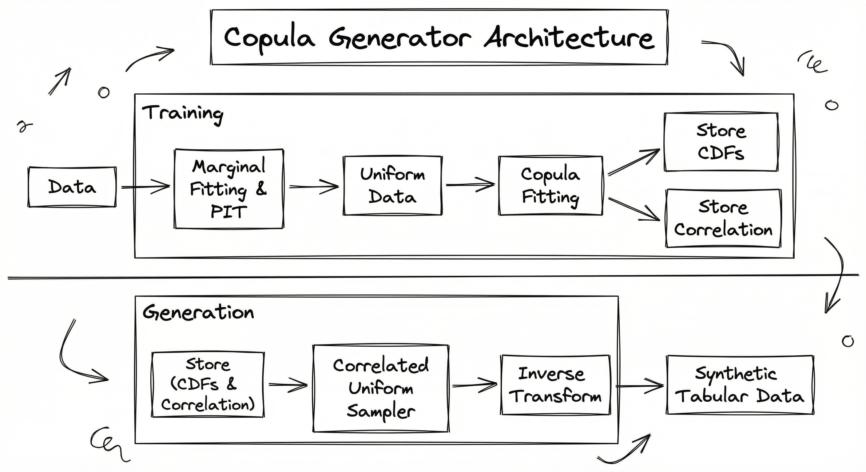
Training Data Flow:

Input ingestion: Load the original tabular dataset (typically a pandas DataFrame) along with metadata specifying column types (numerical, categorical, datetime, ID), primary keys, and any constraints.
Data transformation: Categorical and datetime columns are converted to numerical representations using Reversible Data Transforms (RDTs). Missing values are handled (imputed or flagged).
Marginal fitting: For each numerical column $i$ , fit the best parametric distribution $F_i$ from a candidate set. Store the fitted parameters (mean, std, shape, etc.) and the CDF/inverse-CDF functions.
Probability integral transform: Apply $u_i = F_i(x_i)$ to each column, producing a matrix of uniform $[0,1]$ values.
Normal transform: Apply $\xi_i = \Phi^{-1}(u_i)$ to convert uniforms to standard normals.
Correlation estimation: Compute the $d \times d$ Pearson correlation matrix $\hat{\Sigma}$ of the normal-transformed data. Apply nearest-PSD correction if needed.
Store model: Save the marginal parameters and the correlation matrix (or vine structure for vine copulas).

Generation Data Flow:

Sample correlated normals: Compute Cholesky factor $L$ from $\hat{\Sigma}$ . Draw $\boldsymbol{\epsilon} \sim \mathcal{N}(\mathbf{0}, I)$ and compute $\boldsymbol{z} = L\boldsymbol{\epsilon}$ .
Transform to uniform: Compute $u_i = \Phi(z_i)$ .
Inverse marginal transform: Compute $x_i = F_i^{-1}(u_i)$ using stored marginal parameters.
Reverse data transforms: Convert numerical representations back to original categorical/datetime types.
Post-processing: Enforce min/max bounds, round integer columns, apply any user-specified constraints.
Output: Return synthetic DataFrame with identical schema to the original.

A two-phase architecture diagram. The Training Phase (blue background) shows original tabular data flowing into two parallel paths: marginal fitting (producing stored CDFs) and probability integral transform (converting data to uniform marginals). The uniform data feeds into copula fitting, which stores a correlation matrix or vine structure. The Generation Phase (green background) shows stored copula parameters feeding into a correlated uniform sampler, whose output combines with stored marginal CDFs in an inverse transform step to produce the final synthetic tabular data (green box).

How to Implement

Implementation Approaches

Copula generators can be implemented at three levels of abstraction:

Approach 1: SDV GaussianCopulaSynthesizer -- The highest-level approach. SDV handles metadata detection, data transforms, marginal fitting, copula estimation, and sampling in a single fit() / sample() API. Best for most production use cases. Trains in seconds even on datasets with millions of rows. Supports constraints (unique columns, min/max bounds, regex patterns) and quality evaluation out of the box.

Approach 2: SDV Copulas library -- The mid-level approach. The standalone copulas library (which SDV uses internally) provides direct access to copula objects (GaussianMultivariate, VineCopula), univariate distributions, and visualization tools. Use this when you need more control over the copula fitting process or want to experiment with different copula families.

Approach 3: Manual implementation with scipy/numpy -- The lowest-level approach. Fit marginals with scipy.stats, compute the correlation matrix with numpy, sample with Cholesky decomposition. Use this for educational purposes, custom copula families, or when you cannot install SDV in your environment.

Production Considerations

Copula generators are among the easiest synthetic data methods to productionize:

No GPU required: Training and sampling are CPU-only operations, keeping infrastructure costs minimal (~₹500/month or ~$6 for a cloud VM).
Deterministic training: Unlike GANs, copula fitting is deterministic given the same data. No random initialization, no training instability, no mode collapse.
Fast retraining: When new data arrives, refit the model in seconds. This enables daily or weekly model refresh schedules without significant compute overhead.
Model serialization: The fitted model (marginal parameters + correlation matrix) is compact -- typically under 1 MB even for datasets with hundreds of columns -- and can be stored in any object store or database.
Auditability: Every parameter of the model has a clear statistical interpretation, which is critical for regulatory compliance in banking (RBI guidelines) and insurance (IRDAI requirements).

GaussianCopulaSynthesizer with SDV - Production Example84 lines

from sdv.single_table import GaussianCopulaSynthesizer
from sdv.metadata import SingleTableMetadata
from sdv.evaluation.single_table import evaluate_quality
import pandas as pd
import numpy as np

# Load real data (e.g., loan applications from an Indian NBFC)
real_data = pd.read_csv('loan_applications.csv')
print(f"Real data shape: {real_data.shape}")
print(real_data.head())

# Define metadata
metadata = SingleTableMetadata()
metadata.detect_from_dataframe(real_data)

# Explicitly set column types for accuracy
metadata.update_column('applicant_id', sdtype='id')
metadata.update_column('age', sdtype='numerical', computer_representation='Int64')
metadata.update_column('annual_income_inr', sdtype='numerical', computer_representation='Float')
metadata.update_column('credit_score', sdtype='numerical', computer_representation='Int64')
metadata.update_column('loan_amount_inr', sdtype='numerical', computer_representation='Float')
metadata.update_column('employment_type', sdtype='categorical')
metadata.update_column('city_tier', sdtype='categorical')
metadata.update_column('defaulted', sdtype='boolean')
metadata.set_primary_key('applicant_id')

# Initialize the synthesizer with custom distributions
synthesizer = GaussianCopulaSynthesizer(
    metadata,
    enforce_min_max_values=True,    # Keep values in observed range
    enforce_rounding=True,          # Round to match original precision
    numerical_distributions={
        'annual_income_inr': 'gamma',      # Income is right-skewed
        'credit_score': 'truncnorm',       # Bounded between 300-900
        'loan_amount_inr': 'lognormal',    # Loan amounts are right-skewed
        'age': 'truncnorm',                # Bounded between 18-80
    },
    default_distribution='norm',
)

# Fit the model (typically < 5 seconds for 100K rows)
import time
start = time.time()
synthesizer.fit(real_data)
fit_time = time.time() - start
print(f"Fitting completed in {fit_time:.2f} seconds")

# Inspect the learned correlation matrix
learned_params = synthesizer.get_learned_distributions()
print("\nLearned distributions per column:")
for col, dist_info in learned_params.items():
    print(f"  {col}: {dist_info}")

# Generate synthetic data
num_synthetic = 50_000
synthetic_data = synthesizer.sample(num_rows=num_synthetic)
print(f"\nGenerated {len(synthetic_data)} synthetic rows")
print(synthetic_data.describe())

# Evaluate quality
quality_report = evaluate_quality(
    real_data,
    synthetic_data,
    metadata
)
print(f"\nOverall Quality Score: {quality_report.get_score():.4f}")

# Detailed metrics
shape_details = quality_report.get_details(property_name='Column Shapes')
print("\nColumn Shape Scores:")
print(shape_details)

trend_details = quality_report.get_details(property_name='Column Pair Trends')
print("\nColumn Pair Trend Scores:")
print(trend_details)

# Save model for production deployment
synthesizer.save('models/loan_copula_model.pkl')
print("\nModel saved successfully")

# Load and regenerate later
loaded_synth = GaussianCopulaSynthesizer.load('models/loan_copula_model.pkl')
new_batch = loaded_synth.sample(num_rows=10_000)
print(f"Generated {len(new_batch)} new synthetic rows from saved model")

This example demonstrates the full production workflow for copula-based synthetic data generation using SDV's GaussianCopulaSynthesizer. Key aspects:

Metadata specification: Explicitly defining column types ensures correct handling of numerical vs. categorical columns, IDs, and boolean flags.
Custom distributions: Setting numerical_distributions allows you to specify the best-fitting parametric family for each column. Income and loan amounts are modeled as right-skewed distributions (gamma, log-normal), while bounded values like credit score and age use truncated normals. This significantly improves marginal fit quality.
enforce_min_max_values: Prevents synthetic data from exceeding the observed range of real data -- critical for columns like credit_score (300-900) or age (18-80).
Quality evaluation: SDV's built-in evaluator computes Column Shapes (marginal distribution match) and Column Pair Trends (pairwise correlation preservation), providing a 0-1 quality score.
Model persistence: The fitted model is serialized to a pickle file for deployment. The serialized model contains only marginal parameters and the correlation matrix, making it extremely lightweight.

Manual Gaussian Copula Implementation with scipy/numpy141 lines

import numpy as np
from scipy import stats
from scipy.linalg import cholesky
import pandas as pd

class GaussianCopulaGenerator:
    """Manual Gaussian copula implementation for synthetic data generation."""
    
    def __init__(self):
        self.marginals = {}     # Column name -> fitted distribution
        self.correlation = None  # Correlation matrix in normal space
        self.columns = None
    
    def _fit_marginal(self, data: np.ndarray, col_name: str) -> dict:
        """Fit the best parametric distribution to a single column."""
        candidates = {
            'norm': stats.norm,
            'lognorm': stats.lognorm,
            'gamma': stats.gamma,
            'beta': stats.beta,
            'expon': stats.expon,
        }
        
        best_dist = None
        best_aic = np.inf
        
        for name, dist_class in candidates.items():
            try:
                params = dist_class.fit(data)
                # Compute log-likelihood for AIC
                log_lik = np.sum(dist_class.logpdf(data, *params))
                k = len(params)
                aic = 2 * k - 2 * log_lik
                
                if aic < best_aic:
                    best_aic = aic
                    best_dist = {'name': name, 'class': dist_class, 'params': params}
            except Exception:
                continue
        
        if best_dist is None:
            # Fallback to empirical CDF
            sorted_data = np.sort(data)
            best_dist = {'name': 'empirical', 'sorted_data': sorted_data}
        
        return best_dist
    
    def fit(self, df: pd.DataFrame):
        """Fit the Gaussian copula model to a DataFrame."""
        self.columns = list(df.select_dtypes(include=[np.number]).columns)
        data = df[self.columns].values
        n_samples, n_cols = data.shape
        
        # Step 1: Fit marginal distributions
        print("Fitting marginal distributions...")
        for i, col in enumerate(self.columns):
            col_data = data[:, i]
            col_data = col_data[~np.isnan(col_data)]  # Remove NaNs
            self.marginals[col] = self._fit_marginal(col_data, col)
            print(f"  {col}: {self.marginals[col]['name']}")
        
        # Step 2: Transform to uniform marginals via PIT
        print("Applying probability integral transform...")
        uniform_data = np.zeros_like(data)
        for i, col in enumerate(self.columns):
            marginal = self.marginals[col]
            if marginal['name'] == 'empirical':
                # Use empirical CDF via rank transform
                ranks = stats.rankdata(data[:, i])
                uniform_data[:, i] = ranks / (n_samples + 1)
            else:
                uniform_data[:, i] = marginal['class'].cdf(
                    data[:, i], *marginal['params']
                )
        
        # Clip to avoid infinite values in Phi^{-1}
        eps = 1e-6
        uniform_data = np.clip(uniform_data, eps, 1 - eps)
        
        # Step 3: Transform to normal space
        normal_data = stats.norm.ppf(uniform_data)
        
        # Step 4: Estimate correlation matrix
        self.correlation = np.corrcoef(normal_data, rowvar=False)
        
        # Ensure positive semi-definiteness
        eigvals = np.linalg.eigvalsh(self.correlation)
        if np.min(eigvals) < 0:
            print("  Correcting correlation matrix to nearest PSD...")
            eigvals_corrected = np.maximum(eigvals, 1e-8)
            eigvecs = np.linalg.eigh(self.correlation)[1]
            self.correlation = eigvecs @ np.diag(eigvals_corrected) @ eigvecs.T
            # Re-normalize to correlation matrix
            d = np.sqrt(np.diag(self.correlation))
            self.correlation = self.correlation / np.outer(d, d)
        
        print(f"Fitted copula with {n_cols} columns and {n_samples} samples")
        return self
    
    def sample(self, n_samples: int) -> pd.DataFrame:
        """Generate synthetic samples from the fitted copula model."""
        n_cols = len(self.columns)
        
        # Step 1: Cholesky decomposition
        L = cholesky(self.correlation, lower=True)
        
        # Step 2: Sample independent standard normals
        epsilon = np.random.standard_normal((n_samples, n_cols))
        
        # Step 3: Correlate them
        z = epsilon @ L.T  # Equivalent to L @ epsilon for each sample
        
        # Step 4: Transform to uniform
        u = stats.norm.cdf(z)
        
        # Step 5: Inverse transform to original scale
        synthetic = np.zeros((n_samples, n_cols))
        for i, col in enumerate(self.columns):
            marginal = self.marginals[col]
            if marginal['name'] == 'empirical':
                synthetic[:, i] = np.quantile(
                    marginal['sorted_data'],
                    u[:, i]
                )
            else:
                synthetic[:, i] = marginal['class'].ppf(
                    u[:, i], *marginal['params']
                )
        
        return pd.DataFrame(synthetic, columns=self.columns)


# Usage
df = pd.read_csv('customer_data.csv')

generator = GaussianCopulaGenerator()
generator.fit(df)

synthetic_df = generator.sample(n_samples=10000)
print(f"\nReal data correlations:\n{df[generator.columns].corr().round(3)}")
print(f"\nSynthetic data correlations:\n{synthetic_df.corr().round(3)}")

This manual implementation reveals the inner workings of a Gaussian copula generator. Key educational points:

Marginal fitting: Uses AIC (Akaike Information Criterion) to select the best-fitting parametric distribution from a candidate set. Falls back to empirical CDF if no parametric distribution fits well.
PIT with clipping: The eps clipping prevents Phi^{-1}(0) = $-\infty$ and Phi^{-1}(1) = $+\infty$ , which would corrupt the correlation matrix estimation.
PSD correction: Real-world correlation matrices estimated from finite samples can become non-positive-semidefinite due to numerical errors. The eigenvalue correction projects the matrix to the nearest valid correlation matrix.
Cholesky sampling: The Cholesky decomposition $\Sigma = LL^T$ allows efficient sampling of correlated normals by transforming independent normals: $\boldsymbol{z} = L\boldsymbol{\epsilon}$ .
Inverse transform: Each column uses its own quantile function to convert uniform samples back to the original distribution, preserving marginal shapes while maintaining copula-induced correlations.

Vine Copula with pyvinecopulib for Complex Dependencies80 lines

import pyvinecopulib as pv
import numpy as np
from scipy import stats
import pandas as pd

# Load financial dataset (e.g., daily returns of Indian stocks)
returns = pd.read_csv('nifty50_returns.csv')
columns = ['RELIANCE', 'TCS', 'HDFC_BANK', 'INFOSYS', 'ICICI_BANK']
data = returns[columns].dropna().values

# Step 1: Transform to pseudo-observations (uniform marginals)
# Using empirical CDF via rank transform
n = data.shape[0]
pseudo_obs = np.zeros_like(data)
for j in range(data.shape[1]):
    ranks = stats.rankdata(data[:, j])
    pseudo_obs[:, j] = ranks / (n + 1)  # Avoid 0 and 1

# Step 2: Fit vine copula
# Allow multiple bivariate copula families
controls = pv.FitControlsVinecop(
    family_set=[                    # Candidate bivariate copula families
        pv.BicopFamily.gaussian,    # Symmetric, no tail dependence
        pv.BicopFamily.student,     # Symmetric, tail dependence
        pv.BicopFamily.clayton,     # Lower tail dependence
        pv.BicopFamily.gumbel,      # Upper tail dependence
        pv.BicopFamily.frank,       # Symmetric, light tails
        pv.BicopFamily.joe,         # Upper tail dependence
    ],
    selection_criterion='bic',       # Model selection criterion
    trunc_lvl=3,                     # Truncation level (simplify beyond tree 3)
    tree_criterion='tau',            # Use Kendall's tau for tree structure
)

cop = pv.Vinecop(pseudo_obs, controls=controls)

print(f"Vine copula structure:")
print(f"  Matrix: \n{cop.matrix}")
print(f"  Number of parameters: {cop.npars}")
print(f"  Log-likelihood: {cop.loglik(pseudo_obs):.2f}")

# Print selected families for each pair
for tree in range(min(3, cop.matrix.shape[0] - 1)):
    print(f"\n  Tree {tree + 1}:")
    pair_copulas = cop.get_all_pair_copulas()
    for i, pc_row in enumerate(pair_copulas):
        for j, pc in enumerate(pc_row):
            if pc.family != pv.BicopFamily.indep:
                print(f"    Pair ({i},{j}): {pc.family}, params={pc.parameters}")

# Step 3: Generate synthetic pseudo-observations
n_synthetic = 10000
synthetic_uniform = cop.simulate(n_synthetic, seeds=[42])

# Step 4: Inverse transform to original scale
# Fit marginals using kernel density estimation for flexibility
from scipy.interpolate import interp1d

synthetic_data = np.zeros((n_synthetic, data.shape[1]))
for j in range(data.shape[1]):
    # Build empirical quantile function
    sorted_real = np.sort(data[:, j])
    empirical_quantiles = np.linspace(0, 1, len(sorted_real))
    quantile_fn = interp1d(
        empirical_quantiles, sorted_real,
        bounds_error=False,
        fill_value=(sorted_real[0], sorted_real[-1])
    )
    synthetic_data[:, j] = quantile_fn(synthetic_uniform[:, j])

synthetic_returns = pd.DataFrame(synthetic_data, columns=columns)

# Validate: compare tail dependencies
print("\nReal data tail correlations (lower 5th percentile):")
lower_tail_real = data[data[:, 0] < np.percentile(data[:, 0], 5)]
print(np.corrcoef(lower_tail_real, rowvar=False).round(3))

print("\nSynthetic data tail correlations (lower 5th percentile):")
lower_tail_synth = synthetic_data[synthetic_data[:, 0] < np.percentile(synthetic_data[:, 0], 5)]
print(np.corrcoef(lower_tail_synth, rowvar=False).round(3))

This example shows vine copula modeling for financial returns, where tail dependencies matter critically. Key points:

Pseudo-observations: Instead of fitting parametric marginals, we use the rank transform to create empirical uniform marginals. This is more robust for financial data where parametric distributions may not fit well.
Multiple copula families: The vine copula selects the best bivariate copula for each pair from a candidate set. Clayton copulas capture lower tail dependence (simultaneous crashes), Gumbel captures upper tail dependence (simultaneous rallies), and Student-t captures symmetric tail dependence.
Truncation: Setting trunc_lvl=3 means dependencies beyond the third tree are assumed independent, reducing model complexity without significant loss for most datasets.
Tail validation: The example explicitly checks whether the synthetic data preserves tail correlations -- the correlations that exist during market extremes -- which is where the Gaussian copula famously fails (as demonstrated in the 2008 financial crisis).

Vine copulas are more complex to fit but capture asymmetric and tail-dependent relationships that Gaussian copulas miss entirely.

Configuration Example62 lines

# Copula Generator Configuration (YAML)
model:
  type: gaussian_copula
  version: 1.0

metadata:
  primary_key: customer_id
  columns:
    age:
      sdtype: numerical
      representation: Int64
      distribution: truncnorm
    annual_income:
      sdtype: numerical
      representation: Float
      distribution: lognormal
    credit_score:
      sdtype: numerical
      representation: Int64
      distribution: beta
    loan_amount:
      sdtype: numerical
      representation: Float
      distribution: gamma
    employment_type:
      sdtype: categorical
    city:
      sdtype: categorical
    defaulted:
      sdtype: boolean

copula:
  family: gaussian               # Options: gaussian, vine
  correlation_method: kendall     # Options: pearson, kendall, spearman
  # Vine copula specific settings
  # vine_type: rvine
  # trunc_level: 3
  # bivariate_families:
  #   - gaussian
  #   - student
  #   - clayton
  #   - gumbel
  #   - frank

constraints:
  enforce_min_max: true
  enforce_rounding: true
  custom:
    - type: inequality
      columns: [loan_amount, annual_income]
      relation: loan_amount <= annual_income * 5

generation:
  num_rows: 100000
  batch_size: 10000
  random_seed: 42

evaluation:
  column_shapes: true
  column_pair_trends: true
  ml_efficacy: false
  privacy_score: false

Common Implementation Mistakes

●
Using Pearson correlation directly on non-normal data: The Gaussian copula requires correlation estimation in the normal-transformed space, not the original data space. Computing Pearson correlation on raw (potentially skewed or heavy-tailed) data and using that as the copula correlation matrix will produce incorrect dependency structure. Always apply the PIT and normal transform first, then estimate correlation.
●
Ignoring the positive semi-definite (PSD) requirement: The correlation matrix must be PSD for Cholesky decomposition to work. With many columns or small sample sizes, the estimated matrix may not be PSD due to numerical issues. Always check and apply nearest-PSD correction (e.g., sklearn.covariance.oas or eigenvalue clipping) before sampling.
●
Forgetting to clip uniform values away from 0 and 1: The inverse normal transform $\Phi^{-1}(u)$ diverges to $\pm\infty$ when $u=0$ or $u=1$ . If your PIT produces exact 0s or 1s (common with empirical CDFs at data boundaries), the normal transform will produce infinite values that corrupt everything downstream. Always clip to $[\epsilon, 1-\epsilon]$ with $\epsilon \approx 10^{-6}$ .
●
Assuming Gaussian copula captures tail dependencies: The Gaussian copula has zero tail dependence by construction -- the probability that one variable is extreme given that another is extreme converges to zero. This is dangerous for financial risk modeling where simultaneous extreme events (market crashes, correlated defaults) are the main concern. Use Student-t copula or vine copulas with Clayton/Gumbel components for tail-dependent data.
●
Not validating marginal fits before copula estimation: If the marginal distribution for a column is poorly fitted (e.g., fitting a normal to heavily skewed income data), the PIT will produce non-uniform results, and the copula estimation will be biased. Always inspect Q-Q plots or run KS tests on the PIT-transformed data to verify uniformity before proceeding to copula fitting.
●
Treating categorical columns as numerical: Copula methods are designed for continuous variables. Naively encoding categorical columns as integers (e.g., city=1, 2, 3) and fitting a copula treats them as ordered and continuous, which is wrong. Use proper encoding (one-hot, frequency) or use SDV's built-in RDT transforms that handle mixed types correctly.

When Should You Use This?

Use When

You need fast, reliable synthetic tabular data without GPU infrastructure -- copula generators train in seconds on CPU and produce high-quality data immediately with no training instability
You are working in a regulated industry (banking, insurance, healthcare) where model interpretability and auditability are mandatory -- every parameter of a copula model has a clear statistical meaning
Your dataset has moderate dimensionality (5-100 columns) with primarily numerical features and well-characterized pairwise correlations that need to be preserved
You need to generate privacy-preserving synthetic data for data sharing, model development, or testing where the correlation structure must be maintained but individual records must not be identifiable
You are doing rapid prototyping or need a strong baseline before exploring more complex methods like CTGAN or TVAE -- the Gaussian copula is often the first model to try
Your data has known parametric marginal distributions (e.g., income follows log-normal, counts follow Poisson) that you want to explicitly model rather than learn implicitly
You are building a data pipeline that needs to regenerate synthetic data frequently (daily/weekly) and cannot afford the training time of deep learning methods

Avoid When

Your data has complex, non-linear dependencies that cannot be captured by pairwise correlations -- copulas (especially Gaussian) assume that the full dependency structure is characterized by bivariate relationships
You are working with high-dimensional data (500+ columns) where the correlation matrix becomes ill-conditioned and vine copula fitting becomes combinatorially expensive
Your data contains strong higher-order interactions (e.g., a three-way interaction between age, income, and default that is not captured by any pairwise combination) -- copulas focus on pairwise dependencies
You need to generate non-tabular data such as images, audio, text, or time series with temporal dynamics -- copulas are designed for i.i.d. tabular rows, not sequential or spatial data
Your dataset is predominantly categorical with many high-cardinality categorical columns -- copula methods work best with continuous numerical data and degrade when most columns require extensive encoding
You require differential privacy guarantees out of the box -- while copulas can be combined with DP (e.g., DP noise on the correlation matrix), purpose-built DP synthesizers like DP-CTGAN or PATE-GAN provide stronger formal privacy guarantees
You need to capture tail dependencies (simultaneous extreme events) and are using a Gaussian copula -- the Gaussian copula has zero asymptotic tail dependence by construction, making it unsuitable for extreme risk modeling without switching to vine copulas or Student-t copulas

Key Tradeoffs

Core Tradeoff: Simplicity vs. Expressiveness

The copula generator exists on a spectrum from simple (Gaussian copula) to complex (vine copulas with mixed families). The key tradeoff is between ease of use and interpretability on one end and the ability to capture complex, non-linear, tail-dependent relationships on the other.

Aspect	Gaussian Copula	Vine Copula	CTGAN	TVAE
Training Time	Seconds	Minutes	Hours	Minutes-Hours
GPU Required	No	No	Yes (recommended)	Yes (recommended)
Interpretability	Excellent	Good	Poor	Poor
Tail Dependence	None	Configurable	Implicit	Implicit
High Dimensionality	Good (100s of cols)	Moderate (50-100 cols)	Good (100s of cols)	Good (100s of cols)
Categorical Handling	Via transforms	Via transforms	Native (mode-specific norm)	Native (mode-specific norm)
Correlation Preservation	Excellent (pairwise)	Excellent (inc. conditional)	Good (but noisy)	Good
Marginal Fidelity	Excellent (explicit)	Excellent (explicit)	Good (learned implicitly)	Good (learned implicitly)
Training Stability	Perfect (deterministic)	Perfect (deterministic)	Poor (mode collapse possible)	Good
Regulatory Acceptance	High	High	Low-Medium	Low-Medium

The 2008 Crisis Lesson

The Gaussian copula gained notoriety during the 2008 financial crisis. David X. Li's Gaussian copula model for pricing CDOs assumed that mortgage default correlations were symmetric and had no tail dependence -- meaning the model predicted that the probability of many mortgages defaulting simultaneously was negligibly small. When the housing market crashed, simultaneous defaults occurred at rates the model deemed essentially impossible. The lesson: Gaussian copulas are excellent for modeling normal conditions but dangerous for modeling extreme, simultaneous events. For risk-sensitive applications, always consider vine copulas with tail-dependent bivariate families (Clayton, Gumbel, Student-t).

Cost Comparison

Copula generators are among the cheapest synthetic data methods to deploy:

Method	Training Time (100K rows, 20 cols)	Infrastructure	Monthly Cost (Cloud)	Monthly Cost (INR)
Gaussian Copula	2-5 seconds	CPU only	~₹500 ($6)	₹500
Vine Copula	30-120 seconds	CPU only	~₹500 ($6)	₹500
CTGAN	10-60 minutes	GPU recommended	~₹8,400 ($100)	₹8,400
TVAE	5-30 minutes	GPU recommended	~₹8,400 ($100)	₹8,400
DP-CTGAN	30-120 minutes	GPU required	~₹16,800 ($200)	₹16,800

Practitioner's Tip: Start with GaussianCopulaSynthesizer as your baseline. If the quality score from evaluate_quality() is above 0.85, you likely do not need a more complex method. If pairwise correlations are well-preserved but downstream ML accuracy drops significantly, consider CTGAN or vine copulas for capturing higher-order interactions.

Alternatives & Comparisons

CTGAN

CTGAN uses a conditional GAN architecture specifically designed for tabular data, handling mixed data types and imbalanced categories natively. It can capture more complex, non-linear relationships than a Gaussian copula but requires GPU, takes much longer to train (minutes-hours vs. seconds), and suffers from GAN training instability (mode collapse, convergence issues). Choose copula when you need speed, interpretability, and strong pairwise correlation preservation. Choose CTGAN when you need to capture complex non-linear patterns or your data is heavily categorical.

TVAE

TVAE (Tabular VAE) uses a variational autoencoder architecture for tabular synthesis. It trains more stably than CTGAN and handles mixed types well, but requires a neural network and GPU for best performance. TVAE typically produces slightly lower correlation preservation than copulas but better captures non-linear marginal shapes through its learned encoder. Choose copula for interpretability, speed, and explicit correlation control. Choose TVAE when your marginal distributions are complex and non-parametric, and you can afford the training overhead.

Gaussian Generator

A simple multivariate Gaussian generator assumes all columns follow a joint normal distribution -- both the marginals AND the dependency structure are Gaussian. This is more restrictive than a copula generator, which only uses Gaussian structure for dependencies while allowing arbitrary marginals. Choose the plain Gaussian generator only when all your columns are approximately normally distributed. Choose the copula generator (almost always) when columns have non-Gaussian marginals but you still want to preserve correlations.

GAN Data Generator

General GANs (DCGAN, WGAN-GP, StyleGAN) are designed for unstructured data like images and audio, not tabular data. They require deep learning expertise, GPU infrastructure, and careful hyperparameter tuning. For tabular data, copula generators are almost always a better starting point due to superior interpretability, faster training, and comparable or better correlation preservation. Choose GANs only for image/audio/video synthesis where copulas are not applicable.

Pros, Cons & Tradeoffs

Advantages

Extremely fast training and sampling: A Gaussian copula model trains in 2-5 seconds on 100K rows with 20 columns, and generates 1M synthetic rows in under 10 seconds -- orders of magnitude faster than any deep learning approach
No GPU required: The entire pipeline runs on CPU using standard numpy/scipy operations, making it deployable on any machine including ₹500/month cloud VMs or developer laptops
Fully interpretable and auditable: Every model parameter has a clear statistical meaning -- marginal distribution parameters (mean, variance, shape) and the correlation matrix. Regulators, auditors, and domain experts can inspect exactly how synthetic data is generated
Deterministic and reproducible: Unlike GANs, copula fitting has no random initialization, no adversarial dynamics, and no training instability. Given the same data and random seed, you get identical results every time
Excellent marginal distribution preservation: By explicitly fitting parametric distributions to each column, the marginal fidelity is typically higher than implicit methods (GANs/VAEs) that learn marginals as a side effect of the overall objective
Strong pairwise correlation preservation: The copula directly models the correlation structure, ensuring that pairwise relationships between columns are faithfully reproduced in the synthetic data (quality scores typically 0.85-0.95 on SDV benchmarks)
Modular design: The separation of marginals and dependency structure allows you to independently improve either component -- upgrade a column's marginal from normal to gamma without touching the copula, or switch from Gaussian to vine copula without refitting marginals
Lightweight model serialization: A fitted copula model for 50 columns occupies ~100 KB (marginal parameters + 50x50 correlation matrix), easily stored in databases, version-controlled, or transmitted over networks

Disadvantages

Cannot capture non-linear dependencies: The Gaussian copula reduces all dependencies to linear correlations in the normal space. Complex non-linear relationships (e.g., XOR-like patterns, threshold effects, multi-modal conditional distributions) are lost
No tail dependence in Gaussian copula: The coefficient of asymptotic tail dependence is exactly zero, meaning the model underestimates the probability of simultaneous extreme events -- a critical limitation for financial risk modeling
Struggles with high-cardinality categorical data: Categorical columns must be encoded numerically before copula fitting, and the encoding quality significantly affects results. One-hot encoding inflates dimensionality; frequency encoding loses ordering information
Pairwise-only dependency structure: Standard copulas (including most vine copulas) model dependencies through bivariate relationships. True three-way or higher-order interactions that are not decomposable into pairwise terms are not captured
Sensitive to marginal distribution choice: If you specify a normal distribution for heavily skewed income data, the PIT will produce non-uniform marginals, biasing the copula estimation. Poor marginal fits propagate errors through the entire pipeline
Correlation matrix degrades with dimensionality: For datasets with hundreds of columns and limited samples, the estimated correlation matrix may be poorly conditioned, noisy, or rank-deficient, requiring regularization that can distort the true dependency structure
No built-in privacy guarantees: Unlike DP-GAN or PATE-GAN, a copula generator does not provide formal differential privacy. The correlation matrix and marginal parameters could potentially be inverted to reconstruct individual records, especially with small training datasets

Use SDV's constraint system (sdv.constraints) to enforce business rules during generation. Apply rejection sampling: generate excess rows and filter out those violating constraints. Post-process generated data to clip or adjust violating values. For complex constraints, consider using a constrained optimization step after copula sampling. SDV supports Inequality, Range, FixedCombinations, and custom constraints.

Placement in an ML System

The copula generator sits at the data generation and augmentation stage of an ML pipeline, typically positioned after data collection and validation but before feature engineering and model training.

Primary use case -- synthetic data for development and testing: In many organizations (especially in Indian BFSI), production data cannot leave secure environments. A copula model is fitted on the production data inside the secure environment, and only the model (marginal parameters + correlation matrix, ~100 KB) is exported. Developers and testers then generate unlimited synthetic data from the model on their local machines. This is particularly valuable for teams building credit scoring models, fraud detection systems, or insurance pricing engines where RBI data localization rules restrict data movement.

Secondary use case -- data augmentation for rare events: When your dataset has imbalanced classes (e.g., 1% fraud rate, 0.1% loan defaults), the copula generator can oversample the minority class by fitting a separate copula model to the minority subset and generating additional synthetic minority examples. This is less sophisticated than SMOTE (which operates in feature space) but preserves the full multivariate structure of the minority class.

Integration pattern: The copula generator typically receives cleaned, validated tabular data from an upstream data validator or feature store. The generated synthetic data flows downstream to feature engineering (if used for augmentation) or directly to data consumers (if used for privacy-preserving data sharing). A bias detector should be placed downstream to verify that the synthetic data does not amplify or distort demographic biases present in the original data.

Pipeline Stage

Data Generation & Augmentation

Upstream

data-validator
feature-store

Downstream

feature-engineering
data-splitter
bias-detector

Scaling Bottlenecks

The main scaling bottleneck for Gaussian copula generators is the correlation matrix estimation and Cholesky decomposition, which scale as $O(d^3)$ where $d$ is the number of columns. For datasets with fewer than 200 columns, this is negligible (milliseconds). For 500+ columns, the correlation matrix becomes poorly conditioned and the Cholesky decomposition can become slow (seconds to minutes). The bottleneck is NOT the number of rows -- adding more training rows only linearly increases marginal fitting time. For vine copulas, the bottleneck is tree structure selection, which is $O(d^2)$ per tree and requires fitting $O(d^2)$ bivariate copulas total, each involving parameter estimation. With 100+ columns and rich bivariate families, vine copula fitting can take minutes to hours. Sampling, however, is fast for both methods: $O(n \cdot d^3)$ for Gaussian copula (dominated by Cholesky) and $O(n \cdot d^2)$ for vine copulas (sequential through the tree).

Production Case Studies

J.P. MorganFinancial Services

J.P. Morgan's quantitative research division uses copula-based models extensively for portfolio risk modeling, generating synthetic market data for stress testing and regulatory capital calculations. Their internal tools fit vine copulas to equity, credit, and FX returns to capture tail dependencies across asset classes during market stress events. The approach is favored over GANs because regulators (OCC, Fed) require that the synthetic data generation methodology be fully interpretable and auditable.

Outcome:

Synthetic stress testing datasets generated in minutes rather than weeks of manual scenario construction. Regulatory acceptance of copula-based methodology for internal capital adequacy assessments (ICAAP). Estimated cost savings of $2-5 million annually (approximately ₹16.8 crore to ₹42 crore) in risk data preparation.

Swiss ReInsurance / Reinsurance

Swiss Re's official research page on machine intelligence in insurance, discussing how synthetic data generation (including copula-based methods) helps address data gaps and enables privacy-preserving risk modeling for longevity bonds and mortality dependencies.

Outcome:

Swiss Re Kortis longevity trend bond uses copula models to estimate probability distributions and risk measures; time-varying copula models applied to multi-country mortality data for longevity securitization pricing.

DataCebo / MIT Data to AI LabTechnology / Research

DataCebo, the company behind the Synthetic Data Vault (SDV) library, grew out of MIT's Data to AI Lab research. The GaussianCopulaSynthesizer is SDV's most widely used synthesizer, deployed across healthcare, finance, and government use cases. The team has published extensive benchmarks showing that for single-table tabular data with moderate dimensionality, the Gaussian copula achieves quality scores competitive with CTGAN while training 100-1000x faster.

Outcome:

SDV has been downloaded over 3 million times on PyPI. The GaussianCopulaSynthesizer consistently achieves quality scores of 0.85-0.95 across benchmark datasets. Organizations report 10-50x reduction in time-to-data for development and testing workflows. The Copulas library (standalone) has become the de facto open-source copula implementation for Python.

Reserve Bank of India (RBI) Regulated NBFCsIndian Financial Services

Several Indian Non-Banking Financial Companies (NBFCs) operating under RBI regulations use copula-based generators to create synthetic credit bureau data for model development. Under RBI's data localization and DPDP Act 2023 guidelines, actual credit bureau data (CIBIL, Experian, CRIF) cannot be freely shared across environments. NBFCs fit Gaussian copula models on production credit data and share only the model parameters (not the data) with development teams, who then generate synthetic credit datasets preserving the correlation between variables like annual income, outstanding loan balances, DPD (Days Past Due), and credit utilization ratios.

Outcome:

Compliance with RBI data localization requirements while enabling model development on realistic data. Reduction in credit scoring model development time from 6-8 weeks to 2-3 weeks by eliminating data access bottlenecks. The copula methodology was accepted by external auditors and RBI inspectors due to its statistical transparency.

Tooling & Ecosystem

SDV (Synthetic Data Vault) - GaussianCopulaSynthesizer

PythonOpen Source

The most popular high-level Python library for copula-based synthetic data generation. Provides GaussianCopulaSynthesizer and CopulaGANSynthesizer (a hybrid that uses GAN for marginals and copula for correlations). Handles metadata detection, data transforms, marginal fitting, copula estimation, sampling, and quality evaluation in a unified API. Supports constraints, conditional sampling, and model persistence. Part of the larger SDV ecosystem for single-table, multi-table, and time-series synthesis.

Copulas (sdv-dev/Copulas)

PythonOpen Source

The standalone Python library underlying SDV's copula functionality. Provides direct access to copula objects (GaussianMultivariate, VineCopula), univariate distribution fitting, and visualization tools (1D histograms, 2D scatter plots, 3D scatter plots for comparing real vs. synthetic). Useful when you need lower-level control over the copula fitting process without SDV's full pipeline overhead.

pyvinecopulib

Python (C++ backend)Open Source

A high-performance Python library for vine copula models, providing Python bindings to the C++ vinecopulib header-only library. Supports a wide range of bivariate copula families (Gaussian, Student-t, Clayton, Gumbel, Frank, Joe, BB1, BB6, BB7, BB8), automatic structure selection via maximum spanning trees, and model selection via AIC/BIC. Excels at capturing tail dependencies and asymmetric relationships that Gaussian copulas miss.

Synthia

PythonOpen Source

A Python library for multidimensional synthetic data generation using copulas and functional PCA (fPCA). Uses pyvinecopulib under the hood for vine copula fitting. Particularly designed for geoscientific and climate data but applicable to any tabular data. Provides a clean API for generating synthetic data from vine copula models with support for continuous, discrete, and categorical variables.

copulae (Python)

PythonOpen Source

A Python package for modeling multivariate data using copulas. Supports a comprehensive set of copula families including Gaussian, Student-t, Clayton, Frank, Gumbel, and Archimedean copulas. Provides maximum likelihood estimation, AIC/BIC model selection, and simulation. A good alternative to SDV's Copulas library when you need a broader set of copula families for specialized applications.

VineCopula (R)

ROpen Source

The original and most comprehensive R package for vine copula modeling, developed by the Claudia Czado group at TU Munich. Supports over 40 bivariate copula families, R-vine, C-vine, and D-vine structures, and includes structure selection, parameter estimation, simulation, and diagnostic tools. While R-based, it remains the gold standard for vine copula research and can be called from Python via rpy2.

Research & References

Learning Vine Copula Models For Synthetic Data Generation

Sun, Y., Cuesta-Infante, A., Veeramachaneni, K. (2019)AAAI 2019

Proposes using regular vine copula models for synthetic data generation, formulating vine structure learning with both vector and reinforcement learning representations. Shows that vine copulas outperform Gaussian copulas on synthetic and real-world datasets for capturing complex multivariate dependencies.

Modeling Tabular Data using Conditional GAN

Xu, L., Skoularidou, M., Cuesta-Infante, A., Veeramachaneni, K. (2019)NeurIPS 2019

Introduces CTGAN for synthetic tabular data, the primary deep learning competitor to copula methods. Provides benchmark comparisons showing that CTGAN outperforms Bayesian methods on most real datasets but demonstrates that copula-based methods remain competitive, especially for correlation preservation.

Copula Flows for Synthetic Data Generation

Kamthe, S., Assefa, S., Deisenroth, M. (2021)arXiv preprint

Combines copula theory with normalizing flows: uses copula decomposition to separate marginal and dependency modeling, then applies normalizing flows to learn both components. Shows that copula-flow models capture relationships among mixed variables (continuous and categorical) better than standard copulas or GANs alone.

TVineSynth: A Truncated C-Vine Copula Generator of Synthetic Tabular Data to Balance Privacy and Utility

Griesbauer, T., et al. (2025)AISTATS 2025

Proposes TVineSynth, a vine copula based synthetic data generator that uses the vine tree structure and truncation level to balance the tradeoff between privacy and utility. Demonstrates that truncated vine copulas can achieve competitive utility while providing stronger privacy guarantees than full vine models.

Copula-based transferable models for synthetic population generation

Joshi, H., Drchal, J., Hanna, J., Pechoucek, M. (2023)arXiv preprint

Introduces a copula-based framework for generating synthetic populations that can transfer across different geographic contexts. Uses copulas to model dependency structures that are stable across populations while allowing marginals to vary, enabling synthetic data generation for target populations using models learned from source populations.

Interview & Evaluation Perspective

Common Interview Questions

●
What is Sklar's theorem and why is it foundational to copula-based data generation?
●
Explain the difference between marginal distributions and the copula function. Why is this separation useful?
●
How does the probability integral transform work, and why is it necessary for copula modeling?
●
What is the Gaussian copula's main limitation regarding tail dependence? Give a real-world example where this matters.
●
When would you choose a copula generator over CTGAN for synthetic tabular data?
●
How do vine copulas extend the basic copula framework? What problem do they solve?
●
How would you handle categorical columns in a copula-based synthetic data generator?
●
What happens if the estimated correlation matrix is not positive semi-definite? How do you fix it?
●
How would you evaluate the quality of synthetic data generated by a copula model?

Key Points to Mention

●
Sklar's theorem provides the mathematical foundation: any joint distribution = marginals + copula, uniquely for continuous variables
●
The PIT (probability integral transform) converts any continuous distribution to uniform, enabling standardized dependency modeling
●
Gaussian copula captures dependencies via a correlation matrix in the normal-transformed space -- interpretable, fast, but no tail dependence
●
Vine copulas decompose the joint copula into bivariate building blocks in a tree structure, allowing mixed copula families per pair
●
The 2008 financial crisis demonstrated the danger of Gaussian copula assumptions in tail-risk scenarios
●
SDV's GaussianCopulaSynthesizer is the industry-standard implementation, training in seconds with quality scores of 0.85-0.95
●
Copula models are deterministic and interpretable, making them preferred in regulated industries (banking, insurance, healthcare)

Pitfalls to Avoid

●
Do not conflate the Gaussian copula with assuming all data is Gaussian -- only the dependency structure uses the Gaussian framework, marginals can be anything
●
Do not claim copulas can capture arbitrary complex non-linear relationships -- they are fundamentally limited to pairwise dependency modeling
●
Do not ignore the PSD requirement for correlation matrices -- this is a common source of bugs in manual implementations
●
Do not use copula generators for sequential or spatial data without modification -- they assume i.i.d. rows

Senior-Level Expectation

Senior and staff-level candidates should discuss: (1) the mathematical connection between Sklar's theorem, the PIT, and copula sampling -- not just at a conceptual level but with the ability to derive the sampling algorithm; (2) when and why the Gaussian copula fails (tail dependence = 0, symmetric-only dependencies) and how vine copulas address this with mixed bivariate families; (3) practical production considerations -- model serialization, retraining cadence, constraint enforcement, and integration with data pipelines; (4) privacy implications -- why copula models are NOT differentially private by default and how to add DP guarantees (e.g., adding calibrated noise to the correlation matrix); (5) the relationship to the 2008 financial crisis and the broader lesson about model misspecification in risk-critical systems. The strongest candidates will also discuss alternatives like normalizing flows (copula flows) and the tradeoff between statistical methods and deep generative models for tabular data.

Summary

The copula generator is a mathematically elegant and practically powerful approach to synthetic tabular data generation. Grounded in Sklar's theorem (1959), it separates the modeling problem into two independent parts: per-column marginal distributions (what each column looks like individually) and a copula function (how columns relate to each other). This separation enables explicit, interpretable modeling of both components -- a critical advantage in regulated industries like banking, insurance, and healthcare where auditors need to understand exactly how synthetic data is produced.

The Gaussian copula, which captures dependencies via a correlation matrix in the normal-transformed space, is the most widely used variant. Implemented in SDV's GaussianCopulaSynthesizer, it trains in seconds on CPU, requires no GPU, and achieves quality scores of 0.85-0.95 on standard benchmarks. Its key limitation -- zero tail dependence -- makes it unsuitable for modeling simultaneous extreme events (as famously demonstrated in the 2008 financial crisis). For such scenarios, vine copulas extend the framework with hierarchical bivariate building blocks from tail-dependent families (Clayton, Gumbel, Student-t), offering much richer dependency modeling at the cost of increased complexity.

For ML practitioners, the copula generator should be the default first choice for synthetic tabular data. It is the fastest, cheapest, most interpretable, and most reproducible option available. Start with the Gaussian copula, evaluate quality with SDV's built-in metrics, and only graduate to CTGAN, TVAE, or vine copulas if the quality is insufficient for your downstream use case. In the Indian context, copula generators are particularly well-suited for fintech and BFSI applications where RBI compliance, DPDP Act adherence, and cost efficiency (no GPU infrastructure needed, ~₹500/month operational cost) are primary concerns.

Concept Snapshot

Why This Concept Exists

The Core Problem: Modeling Multivariate Dependencies

Sklar's Insight: Separate the What from the How

From Theory to Practice: The SDV Revolution

Core Intuition & Mental Model

The Recipe Card Analogy

The Probability Integral Transform: The Key Trick

Why Gaussian Copula is the Default

Technical Foundations

Sklar's Theorem

Copula Definition

Probability Integral Transform

Gaussian Copula

Sampling Algorithm

Rank Correlations

Vine Copulas

Internal Architecture

Key Components

Data Flow

How to Implement

Implementation Approaches

Production Considerations

Common Implementation Mistakes

When Should You Use This?

Use When

Avoid When

Key Tradeoffs

Core Tradeoff: Simplicity vs. Expressiveness

The 2008 Crisis Lesson

Cost Comparison

Alternatives & Comparisons

Pros, Cons & Tradeoffs

Advantages

Disadvantages

Failure Modes & Debugging

Correlation Matrix Non-PSD Failure

Marginal Distribution Misfit

Tail Dependency Underestimation

Categorical Encoding Artifacts

Overfitting to Small Samples

Constraint Violation in Generated Data

Placement in an ML System

Pipeline Stage

Upstream

Downstream

Scaling Bottlenecks

Production Case Studies

Tooling & Ecosystem

Research & References

Interview & Evaluation Perspective

Common Interview Questions

Key Points to Mention

Pitfalls to Avoid

Senior-Level Expectation

Summary

Related Blocks & Further Reading

Related ML Blocks

Further Reading