What is TVAE and how does it generate synthetic tabular data?

**TVAE (Tabular Variational Autoencoder)** is a generative model designed specifically for synthesizing realistic tabular data -- structured datasets with rows and columns containing a mix of numerical and categorical values. It was introduced at NeurIPS 2019 alongside CTGAN. TVAE works in two phases: **Training**: The model learns the statistical patterns in your real data. An encoder network compresses each data row into a compact latent representation (a small vector of numbers). A decoder network learns to reconstruct the original row from this compressed representation. The model is trained to minimize a loss function (ELBO) that balances accurate reconstruction against keeping the latent representations well-organized. **Generation**: To create new synthetic data, you sample random vectors from a standard Gaussian distribution and pass them through the trained decoder. The decoder converts each random vector into a realistic-looking data row. Since the latent space is continuous and organized, different random inputs produce diverse but plausible synthetic rows. The key innovation is **mode-specific normalization**: before feeding data to the neural network, each continuous column is analyzed for distinct clusters (modes) using a Gaussian Mixture Model. Values are then encoded relative to their cluster rather than globally. This allows TVAE to capture complex, multimodal distributions like income data with distinct salary bands.

How does TVAE compare to CTGAN? When should I use which?

TVAE and CTGAN were introduced in the same paper and share the same preprocessing (mode-specific normalization) but differ fundamentally in their training approach: **TVAE** uses a **Variational Autoencoder** framework. It trains an encoder-decoder pair by optimizing the ELBO loss function. Training is stable, predictable, and fast. There is no adversarial component. **CTGAN** uses a **Generative Adversarial Network** framework. It trains a generator and discriminator adversarially, with a conditional vector that ensures balanced representation of categorical values. **Choose TVAE when**: - You want reliable, fast training without monitoring for mode collapse - Your data is predominantly continuous with multimodal distributions - You are integrating into automated CI/CD pipelines that cannot tolerate training failures - Your dataset is small to medium (500-100K rows) - You need reproducible results with fixed random seeds **Choose CTGAN when**: - Your dataset has severe class imbalance and you need minority classes well-represented - You need conditional generation (generate data matching specific criteria) - Your data has complex categorical interactions that TVAE's one-hot encoding handles poorly - You can afford to monitor training and tune hyperparameters for maximum quality - Your dataset is large (100K+ rows) where CTGAN's adversarial signal produces noticeably better distributions In practice, many teams start with TVAE as a baseline and switch to CTGAN only when quality metrics justify the additional training complexity.

What is the ELBO loss function and why does TVAE weight it differently?

The **Evidence Lower Bound (ELBO)** is the objective function used to train all Variational Autoencoders, including TVAE. It consists of two terms: **Reconstruction Loss**: Measures how accurately the decoder can reconstruct the original data from the latent code. For TVAE, this includes cross-entropy loss for categorical columns and mode indicators, plus Gaussian negative log-likelihood for normalized continuous values. Higher reconstruction quality means better fidelity in synthetic data. **KL Divergence**: Measures how much the encoder's posterior distribution $q(z|x)$ deviates from the prior $p(z) = \mathcal{N}(0, I)$. Minimizing KL divergence keeps the latent space organized and smooth, enabling meaningful generation by sampling from the prior. The total ELBO is: $\text{ELBO} = \text{Reconstruction} - \text{KL Divergence}$ **TVAE's modification**: The original TVAE implementation multiplies the reconstruction loss by a factor of 2. This is equivalent to a $\beta$-VAE with $\beta = 0.5$, meaning the KL term gets half the relative weight compared to a standard VAE. The effect: TVAE prioritizes **data fidelity** (accurate distributions) over **latent space regularity** (smooth, organized latent codes). For synthetic data generation, this is the right tradeoff -- we care more about the statistical accuracy of generated data than about having a perfectly Gaussian latent space. However, this can lead to overfitting on small datasets, so tuning `loss_factor` is important.

What is mode-specific normalization and how does it work?

**Mode-specific normalization** is the preprocessing technique that makes TVAE (and CTGAN) effective for tabular data. It solves a fundamental problem: real-world continuous columns rarely follow a single Gaussian distribution. Consider a "monthly_salary" column in an Indian dataset. You might see clusters around INR 25,000 (entry-level), INR 60,000 (mid-career), and INR 150,000+ (senior). A single Gaussian with mean ~75,000 would place too much probability around 75,000 (where few people actually earn) and too little at the true peaks. **How it works**: 1. **Fit a Variational Gaussian Mixture Model** (VGM) with $k$ components (default 10) to each continuous column. The Bayesian approach automatically determines how many components are needed -- inactive components get near-zero weight. 2. **For each value**, determine which Gaussian component (mode) it most likely belongs to using posterior probabilities. 3. **Encode the value** as two parts: - **Alpha** ($\alpha$): The normalized position within the assigned mode, computed as $(\text{value} - \mu_\text{mode}) / (4\sigma_\text{mode})$, clipped to $[-1, 1]$ - **Beta** ($\beta$): A one-hot vector indicating which mode the value belongs to 4. **Concatenate** all (alpha, beta) pairs with one-hot encoded categorical columns to form the preprocessed input. **During generation**, the decoder outputs (alpha, beta) predictions. The selected mode provides the mean and standard deviation to denormalize alpha back to the original scale. This encoding means the neural network only needs to predict a small offset within a mode (easy) rather than a raw value on an arbitrary global scale (hard).

How do I evaluate the quality of TVAE-generated synthetic data?

Quality evaluation should cover three dimensions: **fidelity** (does synthetic data match real data distributions?), **utility** (does synthetic data produce equivalent ML model performance?), and **privacy** (does synthetic data protect individual records?). **Fidelity Metrics**: 1. **Column Shapes (KS-test)**: For each continuous column, compute the Kolmogorov-Smirnov statistic between real and synthetic distributions. Score > 0.85 is good. SDV's `evaluate_quality` computes this automatically. 2. **Column Pair Trends**: Measure correlation preservation between all pairs of columns. Compare the correlation matrix of real vs. synthetic data. Score > 0.85 indicates good inter-column relationship preservation. 3. **Visual inspection**: Plot histograms for continuous columns and bar charts for categorical columns, overlaying real and synthetic. Look for mismatched peaks, missing modes, or incorrect category frequencies. **Utility Metrics**: 1. **Train on Synthetic, Test on Real (TSTR)**: Train a classifier (e.g., XGBoost) on synthetic data, test on held-out real data. Compare accuracy/AUC to a model trained on real data. Good synthetic data achieves 85-95% of real data performance. 2. **Train on Real, Test on Synthetic (TRTS)**: The reverse test -- a model trained on real data should perform well on synthetic data if the distributions match. **Privacy Metrics**: 1. **Nearest neighbor distance**: For each synthetic row, find the closest real row. If distances are very small, the model may be memorizing. 2. **Membership inference attack**: Train a classifier to predict whether a given row was in the training set. High attack accuracy indicates privacy leakage. 3. **Novelty score**: Fraction of synthetic rows that are sufficiently different from all training rows (should be > 0.95).

Can TVAE handle missing values and constraints in the data?

**Missing Values**: SDV's `TVAESynthesizer` handles missing values automatically by treating them as a special category. For continuous columns, missing values are assigned their own "mode" in the mode-specific normalization. For categorical columns, NaN/null becomes an explicit category in the one-hot encoding. The model learns when to generate missing values based on the frequency of missingness in the training data. However, if missingness has a complex pattern (e.g., "income is missing when employment_type is 'unemployed'"), TVAE may not capture this conditional relationship perfectly. In such cases, consider imputing strategically before training or using constraint-based generation. **Constraints**: SDV supports several types of constraints that are enforced during or after generation: 1. **Inequality constraints**: Column A > Column B (e.g., end_date > start_date) 2. **Range constraints**: Values must be within specified bounds 3. **Unique constraints**: Generated primary keys must be unique 4. **Custom constraints**: User-defined logic via Python functions Constraints are typically enforced via **reject sampling**: generate rows, reject those violating constraints, repeat until enough valid rows are produced. This is simple but can be slow if constraints are tight (many rejections). For complex multi-column constraints, consider training TVAE on pre-validated data and enforcing constraints post-generation. > **Tip**: Always use `enforce_min_max_values=True` and `enforce_rounding=True` in the `TVAESynthesizer` constructor to prevent generating out-of-range values or inappropriate decimal precision.

What are the computational costs of training and running TVAE?

TVAE is remarkably lightweight compared to other deep generative models. Here are realistic cost estimates: **Training Time** (300 epochs, default parameters): | Dataset Size | Columns | CPU Time | GPU Time | Cloud Cost | |-------------|---------|----------|----------|------------| | 1,000 rows | 15 | 1-2 min | 30 sec | < INR 1 ($0.01) | | 10,000 rows | 30 | 5-10 min | 1-2 min | INR 3 ($0.03) | | 50,000 rows | 30 | 10-20 min | 3-5 min | INR 5 ($0.05) | | 100,000 rows | 50 | 20-40 min | 5-10 min | INR 10 ($0.12) | | 1,000,000 rows | 50 | 1-3 hours | 15-30 min | INR 50 ($0.60) | **Generation Time**: Generating 100K synthetic rows takes 2-10 seconds on GPU, 10-30 seconds on CPU. This is essentially the time for a single decoder forward pass plus inverse preprocessing. **Model Size**: A trained TVAE model is typically 1-10 MB on disk, depending on the number of columns and VGM parameters. Much smaller than image GANs (100+ MB). **Comparison with CTGAN**: TVAE trains 2-5x faster than CTGAN on the same dataset because there is no discriminator to train and no multi-step adversarial updates. For a 50K-row dataset, CTGAN typically takes 30-60 minutes vs. TVAE's 10-20 minutes. **Cloud Cost for Indian Startups**: Using a basic Google Colab GPU (free) or an AWS `g4dn.xlarge` spot instance (~$0.16/hour, ~INR 13/hour), a complete TVAE training run costs less than a cup of chai. Even at enterprise scale (nightly retraining on 1M rows), monthly costs stay under INR 1,500 (~$18).

How does TVAE handle privacy? Can I share TVAE-generated synthetic data safely?

**Standard TVAE does NOT provide formal privacy guarantees.** While synthetic data generated by TVAE is "new" data (not direct copies of training rows), there are real risks: 1. **Memorization**: On small datasets, TVAE can memorize and reproduce training rows, especially with high `loss_factor` and many training epochs. 2. **Attribute inference**: Even if synthetic rows are not exact copies, an attacker might infer sensitive attributes of real individuals by analyzing the synthetic data distribution. 3. **Membership inference**: An attacker with access to the synthetic data and knowledge of the model might determine whether a specific individual was in the training set. **Adding Privacy Guarantees**: 1. **Differential Privacy (DP-TVAE)**: Apply DP-SGD during training -- clip per-sample gradients and add calibrated Gaussian noise. This provides formal $(\epsilon, \delta)$-differential privacy guarantees. Available via libraries like `dp-transformers` or custom implementation. Typical $\epsilon$ values: 1.0 (strong privacy, ~15-25% quality loss), 5.0 (moderate privacy, ~5-10% quality loss), 10.0 (weak privacy, ~2-5% quality loss). 2. **Post-generation privacy auditing**: Run membership inference attacks on the synthetic data to empirically measure privacy leakage. Use SDMetrics or custom attack models. 3. **k-Anonymity verification**: Check that no synthetic row uniquely matches a real individual when projected onto quasi-identifier columns. **Practical Advice for Indian Companies under DPDPA 2023**: Standard TVAE synthetic data is generally safer than direct data sharing, but for regulatory compliance, add DP-TVAE or demonstrate empirically (via privacy audits) that re-identification risk is below an acceptable threshold. Consult legal counsel for specific DPDPA interpretations.

What is the reparameterization trick and why does TVAE need it?

The **reparameterization trick** is a mathematical technique that enables gradient-based training of the VAE encoder. It solves a fundamental problem: how do you backpropagate through a random sampling operation? **The Problem**: During the forward pass, TVAE samples a latent code $z$ from the encoder's output distribution: $z \sim \mathcal{N}(\mu, \sigma^2)$. To train the encoder with gradient descent, we need to compute $\partial \mathcal{L} / \partial \mu$ and $\partial \mathcal{L} / \partial \sigma$. But random sampling is not a differentiable operation -- you cannot compute the gradient of "draw a random number" with respect to the distribution parameters. **The Solution**: Instead of sampling $z \sim \mathcal{N}(\mu, \sigma^2)$ directly, we rewrite the sampling as: $$z = \mu + \sigma \cdot \epsilon, \quad \text{where } \epsilon \sim \mathcal{N}(0, 1)$$ Now $z$ is a **deterministic function** of $\mu$, $\sigma$, and $\epsilon$. The randomness comes from $\epsilon$, which is an external input (not a learned parameter). We can compute gradients with respect to $\mu$ and $\sigma$ using standard backpropagation: $$\frac{\partial z}{\partial \mu} = 1, \quad \frac{\partial z}{\partial \sigma} = \epsilon$$ **Why it matters for TVAE**: Without the reparameterization trick, we would need to use high-variance gradient estimators (like REINFORCE) that make training slow and unstable. The trick enables the entire encoder-decoder pipeline to be trained end-to-end with efficient, low-variance gradients via standard backpropagation.

Data Generation

TVAE in Machine Learning

Q: How does TVAE handle privacy? Can I share TVAE-generated synthetic data safely?

**Standard TVAE does NOT provide formal privacy guarantees.** While synthetic data generated by TVAE is "new" data (not direct copies of training rows), there are real risks: 1. **Memorization**: On small datasets, TVAE can memorize and reproduce training rows, especially with high `loss_factor` and many training epochs. 2. **Attribute inference**: Even if synthetic rows are not exact copies, an attacker might infer sensitive attributes of real individuals by analyzing the synthetic data distribution. 3. **Membership inference**: An attacker with access to the synthetic data and knowledge of the model might determine whether a specific individual was in the training set. **Adding Privacy Guarantees**: 1. **Differential Privacy (DP-TVAE)**: Apply DP-SGD during training -- clip per-sample gradients and add calibrated Gaussian noise. This provides formal $(\epsilon, \delta)$-differential privacy guarantees. Available via libraries like `dp-transformers` or custom implementation. Typical $\epsilon$ values: 1.0 (strong privacy, ~15-25% quality loss), 5.0 (moderate privacy, ~5-10% quality loss), 10.0 (weak privacy, ~2-5% quality loss). 2. **Post-generation privacy auditing**: Run membership inference attacks on the synthetic data to empirically measure privacy leakage. Use SDMetrics or custom attack models. 3. **k-Anonymity verification**: Check that no synthetic row uniquely matches a real individual when projected onto quasi-identifier columns. **Practical Advice for Indian Companies under DPDPA 2023**: Standard TVAE synthetic data is generally safer than direct data sharing, but for regulatory compliance, add DP-TVAE or demonstrate empirically (via privacy audits) that re-identification risk is below an acceptable threshold. Consult legal counsel for specific DPDPA interpretations.

Q: What is the reparameterization trick and why does TVAE need it?

The **reparameterization trick** is a mathematical technique that enables gradient-based training of the VAE encoder. It solves a fundamental problem: how do you backpropagate through a random sampling operation? **The Problem**: During the forward pass, TVAE samples a latent code $z$ from the encoder's output distribution: $z \sim \mathcal{N}(\mu, \sigma^2)$. To train the encoder with gradient descent, we need to compute $\partial \mathcal{L} / \partial \mu$ and $\partial \mathcal{L} / \partial \sigma$. But random sampling is not a differentiable operation -- you cannot compute the gradient of "draw a random number" with respect to the distribution parameters. **The Solution**: Instead of sampling $z \sim \mathcal{N}(\mu, \sigma^2)$ directly, we rewrite the sampling as: $$z = \mu + \sigma \cdot \epsilon, \quad \text{where } \epsilon \sim \mathcal{N}(0, 1)$$ Now $z$ is a **deterministic function** of $\mu$, $\sigma$, and $\epsilon$. The randomness comes from $\epsilon$, which is an external input (not a learned parameter). We can compute gradients with respect to $\mu$ and $\sigma$ using standard backpropagation: $$\frac{\partial z}{\partial \mu} = 1, \quad \frac{\partial z}{\partial \sigma} = \epsilon$$ **Why it matters for TVAE**: Without the reparameterization trick, we would need to use high-variance gradient estimators (like REINFORCE) that make training slow and unstable. The trick enables the entire encoder-decoder pipeline to be trained end-to-end with efficient, low-variance gradients via standard backpropagation.

TVAE (Tabular Variational Autoencoder) is a specialized generative model designed to synthesize realistic tabular data -- the kind of structured, mixed-type data that dominates databases, spreadsheets, and enterprise data warehouses. Introduced alongside CTGAN in the landmark 2019 NeurIPS paper Modeling Tabular Data using Conditional GAN by Lei Xu, Maria Skoularidou, Alfredo Cuesta-Infante, and Kalyan Veeramachaneni at MIT, TVAE adapts the Variational Autoencoder framework to handle the unique challenges of tabular data: mixed continuous and categorical columns, non-Gaussian distributions with multiple modes, and imbalanced class frequencies.

Unlike its adversarial sibling CTGAN, TVAE optimizes a well-defined objective function -- the Evidence Lower Bound (ELBO) -- which decomposes cleanly into a reconstruction term and a KL-divergence regularizer. This gives TVAE a significant practical advantage: stable, predictable training without the mode collapse and gradient instability that plague GAN-based approaches. You do not need to balance a generator against a discriminator, tune critic update schedules, or worry about vanishing gradients. TVAE simply trains an encoder-decoder pair end-to-end, converging reliably in minutes rather than hours.

The key innovation that makes TVAE effective for tabular data is mode-specific normalization. Real-world continuous columns rarely follow a single Gaussian distribution -- income data might have distinct modes for salaried employees, freelancers, and executives; transaction amounts might cluster around common price points. TVAE preprocesses each continuous column using a Variational Gaussian Mixture Model (VGM) to identify modes, then represents each value as a normalized component within its detected mode plus a one-hot indicator of which mode it belongs to. This preprocessing, shared with CTGAN, transforms arbitrarily distributed continuous data into a representation that neural networks can model effectively.

Today, TVAE is a first-class synthesizer in the Synthetic Data Vault (SDV) ecosystem, used by organizations ranging from MAPFRE Insurance to academic medical centers for privacy-preserving data sharing, data augmentation for imbalanced datasets, and rapid prototyping of ML pipelines when real data is unavailable or restricted. For Indian enterprises navigating the Digital Personal Data Protection Act (DPDPA) 2023, TVAE offers a practical path to generating shareable synthetic datasets from sensitive customer, financial, or healthcare records.

Concept Snapshot

What It Is: A Variational Autoencoder adapted for tabular data that encodes mixed-type rows (continuous + categorical columns) into a low-dimensional latent space and decodes them back, learning to generate new synthetic rows that preserve the statistical properties of the original dataset.
Category: Data Generation
Complexity: Intermediate
Inputs / Outputs: Inputs: real tabular dataset with metadata (column types, constraints). Outputs: synthetic tabular dataset of arbitrary size matching the statistical distribution of the real data.
System Placement: Sits in the data generation and augmentation stage of ML pipelines, typically after data cleaning and before feature engineering or model training. Also used as a standalone tool for privacy-preserving data sharing.
Also Known As: Tabular VAE, Tabular Variational Autoencoder, TVAE Synthesizer, VAE for Tabular Data
Typical Users: Data Scientists, ML Engineers, Privacy Engineers, Data Engineers, Compliance Officers, Research Scientists
Prerequisites: Variational Autoencoders (VAE) fundamentals, Evidence Lower Bound (ELBO) and KL divergence, Gaussian Mixture Models basics, Tabular data preprocessing (encoding, normalization), PyTorch or TensorFlow fundamentals
Key Terms: evidence lower bound (ELBO)mode-specific normalizationKL divergencereconstruction losslatent spacereparameterization trickVariational Gaussian Mixtureencoder-decodersynthetic data fidelity

Why This Concept Exists

The Tabular Data Problem

Generative models that work brilliantly on images -- GANs, standard VAEs, diffusion models -- struggle with tabular data. Why? Because tabular data is fundamentally different from images in ways that break standard generative assumptions:

Mixed data types: A single row might contain continuous values (income: 45,000.00), categorical values (city: Mumbai), ordinal values (education: Graduate), and boolean flags (is_active: true). Images are uniformly continuous pixel values.
Non-Gaussian distributions: Income is right-skewed. Age is bounded. Transaction counts are zero-inflated. Standard VAEs assume Gaussian decoders, which produce blurry images but completely wrong tabular distributions.
Multimodal continuous columns: A "transaction_amount" column might have distinct peaks at 99, 499, and 999 (common price points in Indian e-commerce). A single Gaussian cannot capture these modes.
Imbalanced categories: Fraud labels are 0.1% positive. Disease diagnoses are highly skewed. A naive generative model will almost never produce minority class samples.
Complex inter-column dependencies: "salary" correlates with "education" and "city"; "diagnosis" correlates with "age" and "symptoms". These cross-column relationships must be preserved for synthetic data to be useful.

From Standard VAEs to TVAE

Standard Variational Autoencoders -- which encode data into a latent space, regularize with KL divergence against a standard normal prior, and decode back -- produce state-of-the-art results for images. But applying a vanilla VAE to tabular data produces poor results because the Gaussian decoder cannot represent categorical columns, and the assumption of unimodal continuous distributions is violated.

The MIT Data-to-AI Lab, led by Kalyan Veeramachaneni, recognized that the solution required preprocessing innovations rather than architectural overhauls. Their 2019 NeurIPS paper introduced mode-specific normalization: a preprocessing step that transforms each continuous column using a Variational Gaussian Mixture Model (VGM). Each continuous value is encoded as (a) which Gaussian component (mode) it belongs to, and (b) the normalized value within that mode. Categorical columns are simply one-hot encoded.

With this preprocessing, a standard VAE architecture -- multi-layer perceptron encoder and decoder -- can learn tabular distributions effectively. The result is TVAE: a model that is simpler, faster to train, and more stable than CTGAN while achieving competitive or superior statistical fidelity on many benchmark datasets.

The Stability Advantage

The original paper positioned CTGAN as the primary contribution, with TVAE as a baseline comparison. However, practitioners quickly discovered that TVAE's training stability was a decisive advantage in production settings. CTGAN inherits all the training difficulties of GANs: sensitivity to learning rates, potential for mode collapse, and unpredictable training curves. TVAE, by contrast, optimizes a single well-defined loss function (ELBO) with no adversarial dynamics. Training converges reliably, loss curves are interpretable, and hyperparameter sensitivity is far lower.

Indian Context: For Indian fintech companies like Razorpay, PhonePe, and Paytm generating synthetic transaction data under DPDPA 2023 compliance requirements, TVAE's reliable training is a significant operational advantage. You can run TVAE in automated CI/CD pipelines with confidence that it will converge, unlike CTGAN which may require manual monitoring and restart of failed training runs.

Core Intuition & Mental Model

The Compression-and-Reconstruction Game

Imagine you have a large spreadsheet of 50,000 customer records with 30 columns: age, income, city, transaction history, credit score, and so on. TVAE learns to compress each row into a tiny "summary code" (say, 128 numbers) and then reconstruct the original row from that code. The magic is in the compression: TVAE must learn which patterns matter -- the correlations between income and education, the distribution of ages, the frequency of different cities -- because there is not enough room in the 128-number code to store every detail verbatim.

Think of it like a skilled real-estate agent who can describe a property in just a few sentences ("3BHK in Koramangala, 1200 sqft, 15 years old, east-facing, near metro"). From this compressed description, you could reconstruct a plausible listing with reasonable price, amenities, and neighborhood details. The agent learned which features are informative and how they correlate.

The Two Forces: Accuracy vs. Generalization

TVAE balances two competing objectives:

Reconstruction loss: "Can I accurately recreate the original row from the compressed code?" This pushes the model to be precise -- encode all the details, preserve exact distributions.
KL divergence regularization: "Is the compressed code organized in a smooth, standard shape (a Gaussian ball)?" This pushes the model to generalize -- nearby codes should produce similar rows, and you should be able to sample new codes from the Gaussian and get plausible rows.

Without reconstruction loss, the model would produce random nonsense rows. Without KL regularization, the model would memorize training data (codes become scattered, one per training row, and new codes produce garbage). The balance produces a model that generalizes: it understands the data distribution well enough to generate new, plausible rows that never existed in the training set.

Why Mode-Specific Normalization Matters

Here is the key insight that makes TVAE work for tabular data. Suppose you have an "income" column with values like 25,000, 28,000, 30,000 (entry-level salaried), 55,000, 60,000, 65,000 (mid-career), and 150,000, 200,000, 250,000 (senior executives). A single Gaussian would place the mean around 85,000 and spread probability mass uniformly -- generating many incomes around 85,000 that do not actually exist in the real data.

Mode-specific normalization first fits a Gaussian Mixture Model to detect the three clusters. Then each value is encoded as: "I belong to cluster 2 (mid-career), and within that cluster, I am 0.5 standard deviations above the mean." The neural network now only needs to predict (a) which cluster, and (b) a small offset within that cluster -- a much easier problem.

Mental Model: Think of mode-specific normalization as providing "postal codes" for continuous values. Instead of giving a GPS coordinate (one number on a global scale), you say "postal code 560034" (which cluster) and then "200 meters north of the post office" (offset within cluster). The neural network learns to generate valid postal codes and plausible offsets separately.

Technical Foundations

Variational Autoencoder Framework

TVAE consists of two neural networks:

Encoder $q_\phi(\mathbf{z} | \mathbf{r})$ : maps a preprocessed data row $\mathbf{r}$ to a distribution over latent codes $\mathbf{z} \in \mathbb{R}^d$
Decoder $p_\theta(\mathbf{r} | \mathbf{z})$ : maps a latent code $\mathbf{z}$ to a distribution over reconstructed rows $\mathbf{r}$

The encoder outputs parameters of a Gaussian: $q_\phi(\mathbf{z}|\mathbf{r}) = \mathcal{N}(\boldsymbol{\mu}_\phi(\mathbf{r}), \text{diag}(\boldsymbol{\sigma}^2_\phi(\mathbf{r})))$ .

Evidence Lower Bound (ELBO)

Training maximizes the ELBO for each data point $\mathbf{r}_j$ :

$\mathcal{L}(\theta, \phi; \mathbf{r}_j) = \mathbb{E}_{q_\phi(\mathbf{z}|\mathbf{r}_j)}[\log p_\theta(\mathbf{r}_j | \mathbf{z})] - D_{KL}(q_\phi(\mathbf{z}|\mathbf{r}_j) \| p(\mathbf{z}))$

The first term is the reconstruction loss: how well the decoder reconstructs the original row from the latent code. The second term is the KL divergence: how close the encoder's posterior is to the prior $p(\mathbf{z}) = \mathcal{N}(\mathbf{0}, \mathbf{I})$ .

For a standard Gaussian prior, the KL term has a closed-form solution:

$D_{KL}(q_\phi \| p) = -\frac{1}{2} \sum_{k=1}^d \left(1 + \log \sigma^2_k - \mu^2_k - \sigma^2_k \right)$

TVAE-Specific Loss Weighting

In the original TVAE implementation, the reconstruction loss is weighted by a factor of 2 relative to the KL term:

$\mathcal{L}_{TVAE} = 2 \cdot \mathbb{E}_{q_\phi}[\log p_\theta(\mathbf{r}_j | \mathbf{z})] - D_{KL}(q_\phi(\mathbf{z}|\mathbf{r}_j) \| p(\mathbf{z}))$

This upweighting of reconstruction encourages the model to prioritize accurately reproducing column distributions over strictly regularizing the latent space. The factor effectively acts like a $\beta < 1$ in $\beta$ -VAE terminology, trading off some latent space regularity for better data fidelity.

Mode-Specific Normalization (Formal)

For each continuous column $C_i$ , a Variational Gaussian Mixture Model with $k$ components is fitted:

$p(c_i) = \sum_{m=1}^{k} \pi_m \mathcal{N}(c_i; \mu_m, \sigma^2_m)$

where $\pi_m$ are mixing weights. Each value $c_i$ is then represented as a tuple $(\alpha_i, \beta_i)$ :

Mode indicator $\beta_i$ : a one-hot vector of length $k$ indicating which Gaussian component $c_i$ most likely belongs to (computed via posterior $p(m|c_i)$ )
Normalized value $\alpha_i = \frac{c_i - \mu_{m^*}}{4\sigma_{m^*}}$ where $m^* = \arg\max_m p(m|c_i)$ , clipped to $[-1, 1]$

Categorical columns $D_j$ are one-hot encoded. The full preprocessed row becomes:

$\mathbf{r} = [\alpha_1, \beta_1, \alpha_2, \beta_2, \ldots, \alpha_{n_c}, \beta_{n_c}, \text{onehot}(D_1), \ldots, \text{onehot}(D_{n_d})]$

Decoder Output Heads

The decoder uses different output heads for different column types:

Continuous normalized values ( $\alpha_i$ ): Gaussian output with learned mean and variance, or tanh activation
Mode indicators ( $\beta_i$ ): Softmax over $k$ modes (cross-entropy loss)
Categorical columns: Softmax over categories (cross-entropy loss)

The total reconstruction loss is the sum of per-column losses:

$\log p_\theta(\mathbf{r} | \mathbf{z}) = \sum_{i=1}^{n_c} [\log p(\alpha_i | \mathbf{z}) + \log p(\beta_i | \mathbf{z})] + \sum_{j=1}^{n_d} \log p(D_j | \mathbf{z})$

Reparameterization Trick

To backpropagate through the stochastic sampling $\mathbf{z} \sim q_\phi(\mathbf{z}|\mathbf{r})$ , TVAE uses the reparameterization trick:

$\mathbf{z} = \boldsymbol{\mu}_\phi(\mathbf{r}) + \boldsymbol{\sigma}_\phi(\mathbf{r}) \odot \boldsymbol{\epsilon}, \quad \boldsymbol{\epsilon} \sim \mathcal{N}(\mathbf{0}, \mathbf{I})$

This separates the stochastic component ( $\epsilon$ ) from the learned parameters ( $\mu$ , $\sigma$ ), enabling standard gradient-based optimization.

Internal Architecture

TVAE follows the standard encoder-decoder architecture of Variational Autoencoders, with critical adaptations for tabular data. The preprocessing layer handles mode-specific normalization for continuous columns and one-hot encoding for categorical columns, transforming a raw tabular row into a fixed-length vector suitable for neural network processing. The encoder compresses this vector into latent space parameters ( $\mu$ , $\sigma$ ). The sampling layer draws a latent code using the reparameterization trick. The decoder maps the latent code back to a reconstructed row with type-specific output heads.

Both encoder and decoder are multi-layer perceptrons (MLPs) rather than the convolutional architectures used in image VAEs. For tabular data, MLPs are appropriate because there is no spatial locality to exploit -- column ordering is arbitrary. The default SDV implementation uses two hidden layers of 128 units each with ReLU activations, batch normalization, and dropout.

TVAE (Tabular VAE) in ML Systems Architecture — A vertical flowchart showing the TVAE architecture. Raw tabular data enters a Mode-Specific Norma...

During inference (synthetic data generation), only the right half of the diagram is needed: sample $z \sim \mathcal{N}(0, I)$ , decode, and apply inverse mode-specific normalization to produce a synthetic row.

Key Components

Mode-Specific Normalization Preprocessor

Transforms raw continuous columns into bounded, mode-aware representations using Variational Gaussian Mixture Models (VGM). For each continuous column, fits a VGM with $k$ components (default $k=10$ ), identifies the most likely mode for each value, normalizes the value within its mode to $[-1, 1]$ , and creates a one-hot mode indicator vector. This preprocessing converts arbitrarily distributed continuous data into a neural-network-friendly format. Categorical columns are one-hot encoded. The preprocessor stores its fitted parameters (component means, variances, weights) for use in inverse transformation during generation.

Encoder Network

A multi-layer perceptron that maps the preprocessed input vector $\mathbf{r}$ to the parameters of the approximate posterior distribution $q_\phi(\mathbf{z}|\mathbf{r})$ . The default architecture uses two hidden layers with 128 units each, ReLU activations, and batch normalization. The output is split into two heads: $\boldsymbol{\mu}$ (mean) and $\log \boldsymbol{\sigma}^2$ (log-variance) of the latent Gaussian. The encoder learns to compress the high-dimensional preprocessed row into a compact latent representation that captures the essential statistical structure of the data.

Reparameterization Layer

Implements the reparameterization trick: $\mathbf{z} = \boldsymbol{\mu} + \boldsymbol{\sigma} \odot \boldsymbol{\epsilon}$ where $\boldsymbol{\epsilon} \sim \mathcal{N}(0, I)$ . This enables gradient-based optimization by separating the learned parameters from the stochastic sampling. Without this trick, backpropagation through the random sampling step would be impossible, and the encoder could not be trained jointly with the decoder.

Decoder Network

A multi-layer perceptron that maps the latent code $\mathbf{z}$ back to the preprocessed data space. Uses the same architecture as the encoder (two 128-unit hidden layers with ReLU and batch normalization). The output layer splits into type-specific heads: continuous heads produce (alpha, beta) pairs for mode-specific normalized values, and categorical heads produce softmax probabilities over each categorical column's classes. The decoder's output dimensions match the preprocessor's output dimensions.

Loss Function (Weighted ELBO)

Combines reconstruction loss and KL divergence with a 2x weight on reconstruction. The reconstruction loss sums per-column losses: cross-entropy for categorical columns and mode indicators, and Gaussian negative log-likelihood for normalized continuous values. The KL divergence is computed analytically between the encoder's Gaussian and the standard normal prior. The 2x reconstruction weight biases TVAE toward accurately reproducing data distributions at the cost of slightly less regular latent spaces.

Inverse Preprocessing

During generation, converts the decoder's output back to raw data values. For continuous columns: select the predicted mode from the softmax output, denormalize the alpha value using the mode's stored mean and variance, and clip to valid range. For categorical columns: sample from the softmax probability distribution or take argmax. This step bridges the gap between the neural network's internal representation and human-readable tabular data.

Data Flow

Training Flow:

Data ingestion: Load real tabular data and metadata (column types, constraints, primary keys).
Preprocessing: For each continuous column, fit a Variational Gaussian Mixture Model (VGM) to detect modes. Transform values to (alpha, beta) representation. One-hot encode categorical columns. Concatenate into preprocessed vector $\mathbf{r}$ .
Encoding: Pass $\mathbf{r}$ through encoder MLP to get $\mu$ and $\log \sigma^2$ .
Sampling: Draw $\mathbf{z} = \mu + \sigma \cdot \epsilon$ using reparameterization trick.
Decoding: Pass $\mathbf{z}$ through decoder MLP to get reconstructed $\hat{\mathbf{r}}$ .
Loss computation: Compute $\mathcal{L} = 2 \cdot \text{ReconLoss}(\mathbf{r}, \hat{\mathbf{r}}) - D_{KL}(q_\phi \| p)$ .
Backpropagation: Update encoder and decoder parameters via Adam optimizer.
Repeat for the specified number of epochs (default 300).

Generation (Inference) Flow:

Sample latent code: $\mathbf{z} \sim \mathcal{N}(0, I)$ .
Decode: Pass $\mathbf{z}$ through decoder to get $\hat{\mathbf{r}}$ .
Inverse preprocessing: Convert alpha values back to raw continuous values using stored mode parameters. Sample categorical values from softmax outputs.
Post-processing: Apply constraints (e.g., non-negative values, valid date ranges, referential integrity).
Output: Return synthetic tabular row.

Key Difference from CTGAN: TVAE trains end-to-end with a single optimizer and a single loss function. There is no alternating generator-discriminator training, no critic update schedule, and no gradient penalty computation. This makes the training loop dramatically simpler and more predictable.

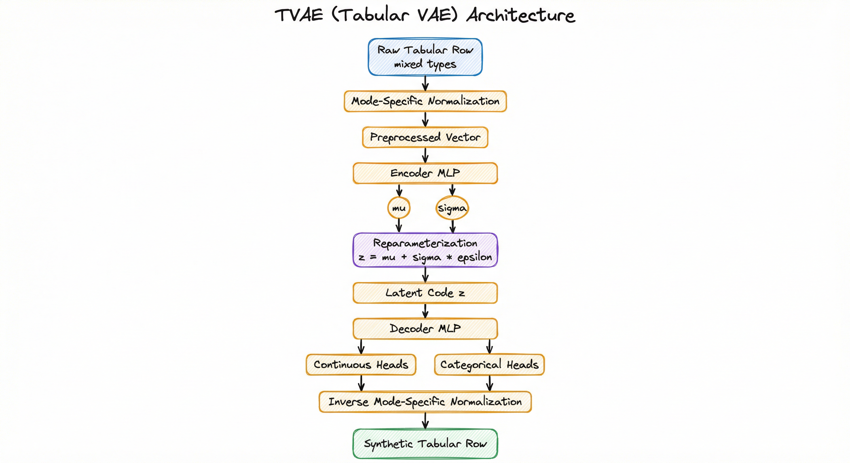
A vertical flowchart showing the TVAE architecture. Raw tabular data enters a Mode-Specific Normalization block (green) that outputs a preprocessed vector. This feeds into the Encoder MLP (blue) which produces mu and sigma parameters. A Reparameterization block (red) samples the latent code z. The Decoder MLP (orange) maps z to continuous heads (alpha, beta values) and categorical heads (softmax probabilities). An Inverse Mode-Specific Normalization step converts these outputs into a final Synthetic Tabular Row (purple).

How to Implement

Implementation Approaches

There are three practical paths to implementing TVAE:

Approach 1: SDV Library (Recommended) -- The Synthetic Data Vault provides the production-grade TVAESynthesizer with metadata-driven configuration, automatic preprocessing, built-in quality evaluation, and constraint handling. This is the standard choice for most production use cases. Install with pip install sdv and configure via the metadata API.

Approach 2: CTGAN Package (Lightweight) -- The standalone ctgan package provides TVAE as a lighter-weight option without the full SDV ecosystem. Useful when you want TVAE without the metadata management overhead. Install with pip install ctgan.

Approach 3: Custom PyTorch Implementation -- For research or when you need architectural modifications (e.g., conditional generation, custom loss functions, different normalization strategies), implement TVAE from scratch in PyTorch. The core architecture is straightforward: two MLPs with the reparameterization trick. The complexity is in the mode-specific normalization preprocessing.

Training Considerations

TVAE training is remarkably simple compared to GANs:

Epochs: Default 300 in SDV. For datasets with <10K rows, 300 is usually sufficient. For 100K+ rows, you may need fewer epochs (150-200) since the model sees more data per epoch.
Batch size: Default 500 in SDV. Larger batches (1000-2000) are fine for large datasets and improve training stability. Smaller batches (128-256) work for small datasets.
Embedding dimension (latent dim): Default 128 in SDV. This controls the capacity of the latent space. For simple datasets (10-15 columns, simple distributions), 64 may suffice. For complex datasets (50+ columns, many modes), increase to 256.
Compression dimensions: The hidden layer sizes of encoder and decoder. Default (128, 128) in SDV. Increase to (256, 256) or (512, 512) for wide datasets with many columns.
L2 regularization (l2scale): Default 1e-5 in SDV. Prevents overfitting on small datasets. Increase to 1e-3 or 1e-4 for very small datasets (<1000 rows).

Cost Note: Training TVAE on a 50K-row, 30-column dataset takes approximately 5-15 minutes on a single CPU and 1-3 minutes on a GPU. Cloud cost is negligible: $0.01-0.05 (~INR 1-4) on a standard instance. Even for large datasets (1M rows), training rarely exceeds 30 minutes on a GPU, costing under$ 0.50 (~INR 42). This is dramatically cheaper than CTGAN which can take 2-10x longer for the same dataset.

TVAE with SDV - Complete Workflow75 lines

from sdv.single_table import TVAESynthesizer
from sdv.metadata import SingleTableMetadata
from sdv.evaluation.single_table import evaluate_quality, run_diagnostic
import pandas as pd

# Load real data
real_data = pd.read_csv('customer_transactions.csv')
print(f"Real data: {real_data.shape[0]} rows, {real_data.shape[1]} columns")

# Define metadata
metadata = SingleTableMetadata()
metadata.detect_from_dataframe(real_data)

# Customize column types
metadata.update_column('customer_id', sdtype='id')
metadata.update_column('age', sdtype='numerical', computer_representation='Int64')
metadata.update_column('income', sdtype='numerical', computer_representation='Float')
metadata.update_column('city', sdtype='categorical')
metadata.update_column('is_fraud', sdtype='boolean')
metadata.update_column('transaction_date', sdtype='datetime',
                       datetime_format='%Y-%m-%d')
metadata.set_primary_key('customer_id')

# Initialize TVAE synthesizer
synthesizer = TVAESynthesizer(
    metadata,
    epochs=300,
    batch_size=500,
    enforce_min_max_values=True,
    enforce_rounding=True,
    embedding_dim=128,
    compress_dims=(128, 128),
    decompress_dims=(128, 128),
    l2scale=1e-5,
    loss_factor=2,  # Reconstruction weight
    verbose=True
)

# Train the model
print("Training TVAE...")
synthesizer.fit(real_data)

# Generate synthetic data
synthetic_data = synthesizer.sample(num_rows=10000)
print(f"Generated {len(synthetic_data)} synthetic rows")
print(synthetic_data.head())

# Evaluate quality
quality_report = evaluate_quality(
    real_data, synthetic_data, metadata
)
print(f"Overall Quality Score: {quality_report.get_score():.4f}")

# Column shapes comparison
column_shapes = quality_report.get_details(property_name='Column Shapes')
print("\nColumn Shape Scores:")
print(column_shapes)

# Column pair trends (correlation preservation)
pair_trends = quality_report.get_details(property_name='Column Pair Trends')
print("\nColumn Pair Trend Scores:")
print(pair_trends)

# Run diagnostic checks
diagnostic = run_diagnostic(
    real_data, synthetic_data, metadata
)
print(f"\nDiagnostic Score: {diagnostic.get_score():.4f}")

# Save model for production use
synthesizer.save('models/tvae_customer.pkl')

# Load and reuse later
loaded_synth = TVAESynthesizer.load('models/tvae_customer.pkl')
new_synthetic = loaded_synth.sample(num_rows=5000)

This is the standard production workflow for TVAE using SDV. Key aspects:

Metadata specification: Explicitly declare column types (numerical, categorical, boolean, datetime, id) for proper preprocessing. Automatic detection works but manual specification is more reliable.
Hyperparameters: epochs=300 (training iterations), embedding_dim=128 (latent space size), compress_dims and decompress_dims (encoder/decoder hidden layers), l2scale=1e-5 (weight regularization), loss_factor=2 (reconstruction weight).
Quality evaluation: evaluate_quality computes Column Shapes (distribution matching via KS-test) and Column Pair Trends (correlation preservation). Scores range from 0 to 1; above 0.85 is good.
Diagnostic checks: Validates data validity (correct types, ranges) and structural integrity (primary keys, constraints).
Model persistence: Save trained models as .pkl files for reuse without retraining.

TVAE from CTGAN Package (Lightweight)53 lines

from ctgan import TVAE
import pandas as pd
import numpy as np

# Load data
real_data = pd.read_csv('loan_applications.csv')

# Define discrete columns explicitly
discrete_columns = [
    'gender', 'education', 'employment_type',
    'loan_status', 'property_area'
]

# Initialize TVAE
model = TVAE(
    embedding_dim=128,
    compress_dims=(128, 128),
    decompress_dims=(128, 128),
    l2scale=1e-5,
    batch_size=500,
    epochs=300,
    loss_factor=2
)

# Train
model.fit(real_data, discrete_columns=discrete_columns)

# Generate synthetic data
synthetic_data = model.sample(5000)

# Validate distributions
for col in real_data.columns:
    if col in discrete_columns:
        # Compare categorical distributions
        real_dist = real_data[col].value_counts(normalize=True)
        synth_dist = synthetic_data[col].value_counts(normalize=True)
        print(f"\n{col}:")
        print(f"  Real:  {dict(real_dist.head())}")
        print(f"  Synth: {dict(synth_dist.head())}")
    else:
        # Compare continuous statistics
        print(f"\n{col}:")
        print(f"  Real  - mean: {real_data[col].mean():.2f}, "
              f"std: {real_data[col].std():.2f}")
        print(f"  Synth - mean: {synthetic_data[col].mean():.2f}, "
              f"std: {synthetic_data[col].std():.2f}")

# Save model
model.save('tvae_loan_model.pkl')

# Load later
loaded = TVAE.load('tvae_loan_model.pkl')
new_samples = loaded.sample(1000)

The standalone ctgan package provides a lighter interface without the full SDV metadata management. You manually specify which columns are discrete/categorical. This approach is useful for quick experiments or when you want to avoid the SDV dependency. The API is simpler but lacks built-in quality evaluation, constraint handling, and metadata validation.

Custom TVAE in PyTorch (Research)210 lines

import torch
import torch.nn as nn
import torch.optim as optim
from torch.utils.data import DataLoader, TensorDataset
from sklearn.mixture import BayesianGaussianMixture
import numpy as np
import pandas as pd


class ModeSpecificNormalizer:
    """Preprocessor that applies mode-specific normalization
    to continuous columns using Variational Gaussian Mixtures."""
    
    def __init__(self, n_components=10):
        self.n_components = n_components
        self.models = {}  # column -> fitted VGM
        self.output_dims = {}  # column -> output dimension
    
    def fit(self, data, continuous_cols, categorical_cols):
        self.continuous_cols = continuous_cols
        self.categorical_cols = categorical_cols
        
        for col in continuous_cols:
            vgm = BayesianGaussianMixture(
                n_components=self.n_components,
                weight_concentration_prior=0.001,
                max_iter=100,
                random_state=42
            )
            values = data[col].values.reshape(-1, 1)
            vgm.fit(values)
            
            # Keep only active components (weight > threshold)
            active = vgm.weights_ > 0.01
            self.models[col] = {
                'vgm': vgm,
                'means': vgm.means_[active].flatten(),
                'stds': np.sqrt(vgm.covariances_[active].flatten()),
                'n_modes': int(active.sum())
            }
            # Output: 1 (alpha) + n_modes (beta one-hot)
            self.output_dims[col] = 1 + self.models[col]['n_modes']
        
        for col in categorical_cols:
            n_cats = data[col].nunique()
            self.models[col] = {
                'categories': data[col].unique().tolist(),
                'n_cats': n_cats
            }
            self.output_dims[col] = n_cats
        
        self.total_dim = sum(self.output_dims.values())
        return self
    
    def transform(self, data):
        outputs = []
        for col in self.continuous_cols:
            info = self.models[col]
            values = data[col].values
            vgm = info['vgm']
            
            # Predict most likely mode for each value
            modes = vgm.predict(values.reshape(-1, 1))
            
            # Normalize within mode
            alpha = np.zeros(len(values))
            beta = np.zeros((len(values), info['n_modes']))
            
            for i, (val, mode) in enumerate(zip(values, modes)):
                mean = info['means'][min(mode, info['n_modes']-1)]
                std = max(info['stds'][min(mode, info['n_modes']-1)], 1e-6)
                alpha[i] = np.clip((val - mean) / (4 * std), -1, 1)
                beta[i, min(mode, info['n_modes']-1)] = 1.0
            
            outputs.append(alpha.reshape(-1, 1))
            outputs.append(beta)
        
        for col in self.categorical_cols:
            info = self.models[col]
            cat_map = {c: i for i, c in enumerate(info['categories'])}
            indices = data[col].map(cat_map).values
            onehot = np.zeros((len(data), info['n_cats']))
            onehot[np.arange(len(data)), indices.astype(int)] = 1.0
            outputs.append(onehot)
        
        return np.concatenate(outputs, axis=1).astype(np.float32)


class TVAEModel(nn.Module):
    """TVAE encoder-decoder model."""
    
    def __init__(self, input_dim, embedding_dim=128,
                 compress_dims=(128, 128),
                 decompress_dims=(128, 128)):
        super().__init__()
        
        # Encoder
        encoder_layers = []
        prev_dim = input_dim
        for dim in compress_dims:
            encoder_layers.extend([
                nn.Linear(prev_dim, dim),
                nn.BatchNorm1d(dim),
                nn.ReLU(),
                nn.Dropout(0.5)
            ])
            prev_dim = dim
        self.encoder = nn.Sequential(*encoder_layers)
        
        self.fc_mu = nn.Linear(prev_dim, embedding_dim)
        self.fc_logvar = nn.Linear(prev_dim, embedding_dim)
        
        # Decoder
        decoder_layers = []
        prev_dim = embedding_dim
        for dim in decompress_dims:
            decoder_layers.extend([
                nn.Linear(prev_dim, dim),
                nn.BatchNorm1d(dim),
                nn.ReLU(),
                nn.Dropout(0.5)
            ])
            prev_dim = dim
        decoder_layers.append(nn.Linear(prev_dim, input_dim))
        self.decoder = nn.Sequential(*decoder_layers)
    
    def encode(self, x):
        h = self.encoder(x)
        return self.fc_mu(h), self.fc_logvar(h)
    
    def reparameterize(self, mu, logvar):
        std = torch.exp(0.5 * logvar)
        eps = torch.randn_like(std)
        return mu + eps * std
    
    def decode(self, z):
        return self.decoder(z)
    
    def forward(self, x):
        mu, logvar = self.encode(x)
        z = self.reparameterize(mu, logvar)
        recon = self.decode(z)
        return recon, mu, logvar


def tvae_loss(recon, original, mu, logvar, loss_factor=2):
    """TVAE loss: weighted reconstruction + KL divergence."""
    # Reconstruction loss (MSE as proxy for Gaussian NLL)
    recon_loss = nn.functional.mse_loss(recon, original, reduction='sum')
    
    # KL divergence
    kl_loss = -0.5 * torch.sum(1 + logvar - mu.pow(2) - logvar.exp())
    
    # TVAE weights reconstruction by loss_factor
    return loss_factor * recon_loss + kl_loss


# Training loop
def train_tvae(data, continuous_cols, categorical_cols,
               epochs=300, batch_size=500, lr=1e-3,
               embedding_dim=128):
    
    # Preprocess
    normalizer = ModeSpecificNormalizer(n_components=10)
    normalizer.fit(data, continuous_cols, categorical_cols)
    processed = normalizer.transform(data)
    
    input_dim = processed.shape[1]
    print(f"Input dimension after preprocessing: {input_dim}")
    
    # Create data loader
    tensor_data = torch.FloatTensor(processed)
    dataset = TensorDataset(tensor_data)
    loader = DataLoader(dataset, batch_size=batch_size, shuffle=True)
    
    # Initialize model
    device = torch.device('cuda' if torch.cuda.is_available() else 'cpu')
    model = TVAEModel(input_dim, embedding_dim).to(device)
    optimizer = optim.Adam(model.parameters(), lr=lr, weight_decay=1e-5)
    
    # Train
    model.train()
    for epoch in range(epochs):
        total_loss = 0
        for batch in loader:
            x = batch[0].to(device)
            recon, mu, logvar = model(x)
            loss = tvae_loss(recon, x, mu, logvar)
            
            optimizer.zero_grad()
            loss.backward()
            optimizer.step()
            total_loss += loss.item()
        
        if (epoch + 1) % 50 == 0:
            avg_loss = total_loss / len(tensor_data)
            print(f"Epoch {epoch+1}/{epochs}, Loss: {avg_loss:.4f}")
    
    return model, normalizer


# Example usage
data = pd.read_csv('customer_data.csv')
continuous_cols = ['age', 'income', 'credit_score']
categorical_cols = ['city', 'education', 'loan_status']

model, normalizer = train_tvae(
    data, continuous_cols, categorical_cols,
    epochs=300, batch_size=500
)

This custom implementation shows the inner workings of TVAE:

ModeSpecificNormalizer: Uses BayesianGaussianMixture from scikit-learn to detect modes in each continuous column. The weight_concentration_prior=0.001 encourages sparsity (few active modes). Each value is encoded as (alpha, beta) where alpha is the normalized offset within a mode and beta is the mode one-hot indicator.
TVAEModel: Standard encoder-decoder with batch normalization and dropout. The encoder maps preprocessed rows to (mu, logvar), the reparameterization trick enables backpropagation through sampling, and the decoder reconstructs the preprocessed row.
Loss function: The loss_factor=2 upweights reconstruction over KL divergence, matching the original TVAE paper. This biases toward accurate data reproduction rather than smooth latent space structure.
Training: Simple end-to-end optimization with Adam. No adversarial dynamics, no critic updates, no gradient penalties. Loss decreases monotonically (barring noise), making it easy to diagnose training problems.

Configuration Example39 lines

# TVAE Configuration (YAML)
model:
  type: tvae
  embedding_dim: 128
  compress_dims: [128, 128]
  decompress_dims: [128, 128]
  l2scale: 1e-5
  loss_factor: 2

training:
  epochs: 300
  batch_size: 500
  learning_rate: 1e-3
  optimizer: adam
  weight_decay: 1e-5
  early_stopping: false

preprocessing:
  mode_specific_normalization:
    n_components: 10
    weight_concentration_prior: 0.001
  enforce_min_max: true
  enforce_rounding: true

evaluation:
  metrics:
    - column_shapes    # KS-test per column
    - column_pairs     # Correlation preservation
    - diagnostic       # Data validity checks
  downstream_test:
    model: xgboost
    metric: auc
    n_splits: 5

output:
  num_rows: 10000
  format: csv
  save_model: true
  model_path: models/tvae_trained.pkl

Common Implementation Mistakes

●
Not specifying column types in metadata: TVAE treats continuous and categorical columns completely differently (mode-specific normalization vs. one-hot encoding). If a categorical column like zipcode or product_id is auto-detected as numerical, TVAE will fit a Gaussian Mixture to it, producing nonsensical synthetic values. Always explicitly declare column types in metadata.
●
Using default hyperparameters for all datasets: The default compress_dims=(128, 128) works for datasets with 10-30 columns, but for wide datasets (100+ columns) the model capacity is insufficient. Conversely, for very small datasets (<500 rows) with few columns, the default capacity causes overfitting. Scale hidden layer sizes proportionally to data complexity.
●
Ignoring the loss_factor parameter: TVAE's loss_factor=2 upweights reconstruction loss. Changing this dramatically affects model behavior: higher values produce more accurate but potentially overfit synthetic data; lower values (e.g., 1) produce more diverse but less accurate data. Treat this as a critical hyperparameter, not a fixed constant.
●
Training too many epochs on small datasets: With 500-1000 rows, 300 epochs of TVAE training leads to overfitting -- the model memorizes training rows rather than learning the distribution. For small datasets, reduce to 50-100 epochs and increase l2scale to 1e-3 for stronger regularization.
●
Expecting TVAE to handle high-cardinality categorical columns well: Columns with 1000+ unique categories (e.g., product IDs, full addresses) bloat the one-hot encoding and overwhelm the model. Preprocess high-cardinality categoricals: group rare categories into 'Other', use embeddings, or drop entirely if not needed.
●
Not evaluating synthetic data quality: Generating data without validation is dangerous. Always compute distribution similarity (KS-test for continuous, chi-square for categorical), correlation preservation, and downstream model performance. SDV's evaluate_quality and run_diagnostic methods make this easy.

When Should You Use This?

Use When

You need stable, predictable training for synthetic tabular data generation without the risk of mode collapse or training divergence that plagues GAN-based approaches
Your dataset is small to medium-sized (500-100K rows) where TVAE's training efficiency and lower data requirements provide an advantage over CTGAN
Your data has predominantly continuous features -- TVAE's mode-specific normalization excels at capturing multimodal continuous distributions (income levels, transaction amounts, sensor readings)
You need fast iteration cycles for experimentation or CI/CD integration -- TVAE trains 2-5x faster than CTGAN on the same dataset and converges reliably without manual monitoring
You want a well-defined loss function (ELBO) that provides interpretable training curves -- unlike GAN losses, TVAE loss decreases monotonically and lower is better
You're generating synthetic data for privacy-preserving data sharing under regulations like DPDPA (India), GDPR, or HIPAA, and need a reliable baseline synthesizer
Your team has limited deep learning expertise and needs a model that works out-of-the-box with minimal hyperparameter tuning compared to adversarial approaches
You need reproducible training outcomes -- TVAE with a fixed random seed produces deterministic results, unlike GANs where training outcomes vary across runs

Avoid When

Your dataset is predominantly categorical with many high-cardinality columns -- TVAE's one-hot encoding creates prohibitively large input vectors and the model struggles with complex categorical interactions
You need the highest possible statistical fidelity on complex multivariate distributions -- CTGAN often produces higher-fidelity synthetic data on large, complex datasets due to its adversarial training signal
Your dataset has severe class imbalance (e.g., 0.1% fraud) and you need the minority class well-represented -- TVAE tends to under-represent rare categories and may ignore minority modes entirely
You require conditional generation (e.g., generate only rows where city=Mumbai and income>100000) -- CTGAN's conditional vector natively supports this, while TVAE generates unconditionally and requires post-filtering
Your data has complex relational structure (multiple linked tables with foreign keys) -- consider SDV's multi-table models (HMA, PAR) rather than single-table TVAE
You need explicit density estimation or likelihood values for anomaly scoring -- while TVAE's decoder defines a likelihood model, the ELBO only provides a lower bound and is not suitable for precise density estimation

Key Tradeoffs

Core Tradeoff: Stability vs. Fidelity

TVAE trades some statistical fidelity for dramatically better training stability. On benchmarks from the original paper, CTGAN achieved slightly higher scores on 3 of 7 datasets, while TVAE was competitive or better on the remaining 4. However, TVAE never fails to train -- it converges reliably every time -- while CTGAN training can fail due to mode collapse or divergence, requiring restarts and hyperparameter tuning.

Aspect	TVAE	CTGAN	Gaussian Copula
Training Stability	Excellent	Moderate (mode collapse risk)	Excellent
Statistical Fidelity	Good (0.85-0.95 quality)	Very Good (0.88-0.97 quality)	Moderate (0.75-0.90 quality)
Training Time (50K rows)	5-15 min	15-60 min	1-3 min
Continuous Distributions	Excellent (mode-specific)	Excellent (mode-specific)	Good (Gaussian assumption)
Categorical Distributions	Moderate	Good (conditional vector)	Good (direct modeling)
Class Imbalance Handling	Poor	Good (conditional training)	Moderate
Hyperparameter Sensitivity	Low	High	Very Low
Conditional Generation	Not native	Native (conditional vector)	Not native

Cost Comparison

Dataset Size	TVAE Time	TVAE Cost (Cloud)	CTGAN Time	CTGAN Cost
1K rows, 15 cols	1-2 min	$0.01 / INR 1	5-10 min	$0.05 / INR 4
10K rows, 30 cols	3-8 min	$0.03 / INR 3	15-30 min	$0.15 / INR 13
50K rows, 30 cols	5-15 min	$0.05 / INR 4	30-60 min	$0.50 / INR 42
100K rows, 50 cols	10-25 min	$0.10 / INR 8	1-3 hours	$1.50 / INR 126
500K rows, 100 cols	20-45 min	$0.25 / INR 21	3-8 hours	$4.00 / INR 336

Practitioner's Recommendation: Start with TVAE for initial experiments and baseline synthetic data. If quality metrics are insufficient (quality score <0.85), switch to CTGAN for the specific dataset. For production pipelines where reliability is critical, prefer TVAE unless CTGAN's quality advantage is demonstrably significant for your use case.

Alternatives & Comparisons

CTGAN

CTGAN uses adversarial training (generator + discriminator) instead of TVAE's ELBO optimization. CTGAN generally achieves slightly higher statistical fidelity on complex datasets, especially those with severe class imbalance (thanks to its conditional vector that ensures minority categories are generated). However, CTGAN's training is less stable -- it can suffer mode collapse and requires careful hyperparameter tuning. Choose CTGAN when you need the highest quality on a specific dataset and can afford to monitor training. Choose TVAE when you need reliable, fast training without manual oversight.

VAE Generator

Standard VAE Generator works on continuous data (images, audio) but lacks TVAE's mode-specific normalization for tabular data. Applying a vanilla VAE to mixed-type tabular data produces poor results because the Gaussian decoder cannot model categorical columns or multimodal continuous distributions. Choose standard VAE for image/audio generation. Choose TVAE specifically for tabular data.

Copula Generator

Gaussian Copula synthesizers model marginal distributions independently and capture dependencies via a copula function. They train faster than TVAE (seconds vs. minutes) and work well for simple, low-dimensional datasets. However, copulas assume Gaussian dependencies and struggle with complex non-linear relationships between columns. Choose Copula Generator for simple datasets or as a fast baseline. Choose TVAE when you need to capture non-linear dependencies and multimodal distributions.

GAN Generator

General GAN architectures (DCGAN, StyleGAN) are designed for image and unstructured data, not tabular data. Applying standard GANs to tables requires significant architectural adaptation. CTGAN and TVAE exist precisely because generic GANs fail on tabular data. Choose GAN Generator for image synthesis, style transfer, or unstructured data. Choose TVAE for structured tabular data.

SMOTE

SMOTE creates synthetic samples by interpolating between existing minority class samples in feature space. It is specifically designed for class imbalance and does not learn the data distribution holistically. SMOTE is simpler, faster, and effective for oversampling minority classes in classification tasks. However, it cannot generate entirely new datasets, does not handle categorical features natively (SMOTE-NC variant exists), and interpolated samples may not be realistic. Choose SMOTE for targeted class balancing in a specific ML task. Choose TVAE for full synthetic dataset generation with all column types.

Pros, Cons & Tradeoffs

Advantages

Stable, predictable training: TVAE optimizes a well-defined ELBO objective with no adversarial dynamics. Training converges reliably without mode collapse, vanishing gradients, or oscillating losses. You can train TVAE in automated pipelines with confidence it will succeed.
Fast training and inference: TVAE trains 2-5x faster than CTGAN on equivalent datasets because there is no discriminator to maintain and no multi-step critic updates. A 50K-row dataset trains in 5-15 minutes on CPU. Generation is a single decoder forward pass -- 100K synthetic rows in seconds.
Interpretable loss curves: Unlike GAN losses which oscillate and do not correlate with sample quality, TVAE's ELBO loss decreases monotonically and directly reflects reconstruction accuracy. Lower loss means better synthetic data. This makes debugging and early stopping straightforward.
Effective mode-specific normalization for continuous features: TVAE excels at capturing multimodal continuous distributions (income levels, transaction amounts, sensor readings) thanks to VGM-based preprocessing. Each mode is modeled independently, preserving cluster structure.
Low hyperparameter sensitivity: Default TVAE parameters work well across a wide range of datasets. Unlike CTGAN where wrong learning rates or critic steps cause catastrophic failure, TVAE degrades gracefully with suboptimal settings.
Latent space structure: The VAE framework produces a smooth, organized latent space where nearby points decode to similar rows. This enables latent space interpolation and potentially useful representations for downstream tasks.
Production-ready via SDV: The TVAESynthesizer in SDV provides metadata management, quality evaluation, constraint handling, and model persistence. No custom engineering needed for standard use cases.
Reproducible results: With a fixed random seed, TVAE produces identical synthetic data across runs. This is critical for regulated environments where reproducibility is required.

Disadvantages

Weaker on complex categorical interactions: TVAE uses one-hot encoding for categorical columns, which does not capture interactions between categories well. CTGAN's conditional vector training explicitly conditions on categorical values, producing more accurate categorical distributions, especially for imbalanced classes.
Minority class under-representation: TVAE trains by sampling uniformly from all rows, so rare categories (e.g., fraud labels at 0.1%) are seen rarely during training and are under-represented in synthetic data. CTGAN's training-by-sampling approach explicitly addresses this.
No native conditional generation: TVAE generates data unconditionally from the prior $p(z)$ . To generate data matching specific conditions (e.g., only Mumbai customers with income > 100K), you must generate excess data and filter -- wasteful and impractical for rare conditions. CTGAN natively supports conditional generation.
Standard normal prior assumption: The fixed prior $p(z) = \mathcal{N}(0, I)$ may not match the true latent structure of complex data, causing the model to spread probability mass over implausible regions. More expressive priors (GMM, normalizing flows) could help but are not in the standard TVAE.
Reconstruction loss weighting sensitivity: The loss_factor=2 is hardcoded in the original implementation and can impair performance on certain datasets. There is no principled method to set this value -- it requires empirical tuning per dataset.
High-cardinality categorical columns bloat input: Columns with 500+ categories create massive one-hot vectors that dominate the input, drowning out signal from continuous columns. This is a fundamental limitation of the one-hot encoding approach.
Limited privacy guarantees without extensions: Standard TVAE provides no formal privacy guarantees. Synthetic rows may closely resemble training rows, risking re-identification. Differential privacy extensions (DP-TVAE) exist but significantly degrade data quality.

Use KL annealing (cyclical or linear): start with the KL term weighted at 0 and gradually increase to 1 over the first 50-100 epochs, forcing the model to use the latent space before regularizing it. Reduce decoder capacity (fewer layers or units) so it cannot reconstruct without leveraging the latent code. Increase latent dimension to provide more capacity for encoding information. Use free bits: set a minimum KL per dimension (e.g., 0.1 nats) below which the KL penalty is not applied.

Placement in an ML System

Where TVAE Fits in Production ML Systems

TVAE occupies the synthetic data generation layer in an ML pipeline, sitting between data collection/cleaning and downstream model training or data sharing:

Data Collection: Gather real-world tabular data (customer records, transactions, medical records, sensor readings).
Data Cleaning: Handle missing values, remove duplicates, validate data types, apply business rules.
Data Validation: Verify schema, distributions, and quality before training TVAE.
TVAE Training: Fit TVAE on the cleaned, validated dataset. Store the trained model artifact.
Synthetic Generation: Generate synthetic datasets of desired size from the trained model.
Quality Evaluation: Run statistical tests (KS-test, chi-square), correlation checks, and downstream ML performance benchmarks.
Privacy Auditing: Run membership inference attacks, assess re-identification risk, verify compliance.
Downstream Use: Serve synthetic data for (a) ML model training/validation, (b) privacy-preserving data sharing, (c) development/testing environments, or (d) data augmentation.

Integration Patterns

Pattern 1: CI/CD Synthetic Data Pipeline -- Train TVAE nightly on production data snapshots. Generate fresh synthetic datasets for development and testing environments. Developers never touch real customer data.

Pattern 2: Privacy-Preserving Data Sharing -- Train TVAE on sensitive data within the secure enclave. Generate synthetic data and share with external partners (researchers, vendors, regulators). Common in healthcare (hospital sharing data with pharmaceutical companies) and finance (banks sharing data with fintechs).

Pattern 3: Data Augmentation for Imbalanced Classes -- Use TVAE to generate additional training samples, particularly for underrepresented classes, before feeding into a downstream classifier. Combine real and synthetic data in a controlled ratio (e.g., 80% real, 20% synthetic).

Indian Enterprise Example: A leading Indian private bank uses TVAE in their ML platform to generate synthetic customer transaction data. Development and QA teams use synthetic data for testing new features, eliminating the need for access to real customer data and simplifying DPDPA compliance. The synthetic data pipeline runs nightly, generating 500K rows in under 30 minutes, costing approximately INR 5 per run on their internal GPU cluster.

Pipeline Stage

Data Generation / Augmentation

Upstream

data-validation
feature-store

Downstream

data-validation
feature-store
differential-privacy

Scaling Bottlenecks

Training Bottlenecks

TVAE training is compute-light compared to GANs and diffusion models. The primary bottleneck is the mode-specific normalization preprocessing: fitting VGMs for each continuous column scales as $O(n \cdot k \cdot \text{iter})$ where $n$ is the number of rows, $k$ is the number of components, and iter is the VGM EM iterations. For 1M rows with 50 continuous columns, preprocessing alone takes 2-5 minutes.

The neural network training is standard MLP forward/backward passes. With batch size 500 and 128-dim hidden layers, each epoch processes all data in a single pass through memory-efficient minibatches. Memory is the main constraint: the preprocessed data matrix (with mode-specific normalization and one-hot encoding) can be 5-20x wider than the original data. A dataset with 30 columns and 10 components per continuous column plus categorical one-hots might expand to 500+ dimensions.

Inference (Generation) Bottlenecks

Generation is extremely fast: sample $z \sim \mathcal{N}(0, I)$ and run a single decoder forward pass. Generating 1M synthetic rows takes ~10-30 seconds on a GPU, limited mainly by the inverse preprocessing step (converting alpha/beta back to raw values). For batch generation at scale, the bottleneck shifts to I/O: writing 1M rows to CSV or loading into a database.

Scaling to Large Datasets

For datasets with 10M+ rows, the main challenge is preprocessing memory: the expanded preprocessed matrix may not fit in RAM. Solutions: (1) fit VGMs on a stratified sample (100K rows), then transform in chunks; (2) use streaming data loaders that preprocess on-the-fly during training; (3) reduce n_components to limit expansion factor. The neural network training itself scales linearly with data size and handles 10M rows comfortably in 1-2 hours on a GPU.

Production Case Studies

MAPFRE InsuranceInsurance

MAPFRE, one of the world's largest insurance companies, used SDV's synthetic data generation (including TVAE and CTGAN) to augment their fraud detection training data. Their real fraud dataset was severely imbalanced -- fraudulent claims represented a tiny fraction of total claims. By generating synthetic fraudulent claims that preserved the statistical characteristics of real fraud patterns, they significantly improved their AI-driven fraud detection model's ability to identify suspicious homeowner insurance claims.

Outcome:

MAPFRE improved their fraud detection rate by 31% using synthetic data augmentation. The synthetic data preserved key correlations between claim attributes (amount, timing, claimant history, property details) while providing the volume needed to train robust classifiers. The SDV-based pipeline reduced dataset preparation time from weeks to days.

DataCebo / SDV EcosystemSynthetic Data Platform

DataCebo, the company behind the Synthetic Data Vault, has built an enterprise platform around TVAE and CTGAN. Spun out of MIT's Data-to-AI Lab in 2020, DataCebo provides production-grade synthetic data generation for enterprises across healthcare, finance, insurance, and government. Their platform adds enterprise features on top of the open-source SDV: automated quality evaluation, privacy auditing, constraint enforcement for relational databases, and integration with data catalogs.

Outcome:

SDV has been downloaded over 5 million times and is used by 100+ organizations worldwide. The library supports single-table (TVAE, CTGAN, Gaussian Copula), multi-table (HMA), and sequential data (PAR) synthesis. DataCebo's enterprise customers report 40-60% reduction in time spent on data preparation for ML projects.

Frontiers in Digital Health (Healthcare Research)Healthcare

A comprehensive evaluation framework published in Frontiers in Digital Health (2025) assessed TVAE alongside CTGAN, Gaussian Copula, and other synthesizers on medical datasets including cardiovascular disease records and clinical trial data. The study evaluated fidelity, utility, and privacy dimensions. TVAE demonstrated strong column-wise fidelity (KS-statistic 0.90) and row-wise correlation preservation (Pearson 0.97) while maintaining high synthesis novelty (0.999), indicating that generated records were not copies of training data.

Outcome:

TVAE achieved the fastest training time (401 seconds) among deep learning synthesizers tested, while maintaining competitive fidelity. The study found that adding differential privacy to DP-TVAE had a neutral impact on fidelity for certain medical datasets, suggesting TVAE as a viable privacy-preserving synthesizer for healthcare data sharing under HIPAA and GDPR.

Anti-Money Laundering (Banking)Financial Services

A major bank used SDV's synthetic data generators (including TVAE) to create synthetic transaction datasets for training anti-money laundering (AML) models. Real transaction data could not be shared across departments or with external model vendors due to privacy regulations. TVAE generated synthetic transaction records preserving the statistical patterns of legitimate and suspicious transactions -- transaction amounts, frequencies, counterparty relationships, and temporal patterns -- while ensuring no real customer data was exposed.

Outcome:

The synthetic data enabled cross-team ML model development without privacy violations. AML models trained on synthetic data achieved comparable detection rates to models trained on real data, validating the utility of TVAE-generated synthetic transactions. The bank estimated annual savings of $200,000-500,000 (~INR 1.68-4.2 crore) in compliance and data governance costs.

Tooling & Ecosystem

Synthetic Data Vault (SDV)

PythonOpen Source

The primary production-grade library for TVAE. Provides TVAESynthesizer with metadata-driven configuration, automatic preprocessing (mode-specific normalization), built-in quality evaluation (evaluate_quality, run_diagnostic), constraint handling, and model persistence. Supports single-table, multi-table, and sequential data synthesis. The standard tool for tabular synthetic data.

CTGAN Package

PythonOpen Source

Standalone package providing both TVAE and CTGAN classes without the full SDV ecosystem. Lighter weight than SDV (fewer dependencies) but requires manual column type specification and lacks built-in quality evaluation. Good for quick experiments and custom pipelines where you handle metadata yourself.

Synthcity

PythonOpen Source

Open-source synthetic data library from the van der Schaar Lab (Cambridge) that includes TVAE alongside 20+ other generators (CTGAN, normalizing flows, diffusion models, Bayesian networks). Provides unified benchmarking across generators with consistent evaluation metrics. Useful for comparing TVAE against alternatives on your specific dataset.

YData Fabric

PythonCommercial

Commercial synthetic data platform that includes TVAE-based synthesizers alongside proprietary models. Provides automated data profiling, no-code and SDK options, quality reports, and privacy guarantees. YData achieved the top ranking in AIMultiple's 2025 synthetic data benchmark. Available as cloud service or on-premise deployment.

Gretel Synthetics

PythonOpen Source

Open-source library from Gretel.ai supporting tabular synthetic data generation with differential privacy. Includes VAE-based and LSTM-based synthesizers alongside GAN variants. The commercial Gretel platform adds GUI-based training, privacy auditing, and CI/CD integration. Strong focus on privacy-preserving synthetic data for regulated industries.

SDMetrics

PythonOpen Source

Dedicated evaluation library for synthetic tabular data. Computes column-level metrics (KS-test, chi-square), pair-level metrics (correlation preservation), and diagnostic checks (data validity, structural integrity). Works with any synthetic data generator, not just SDV. Essential for validating TVAE output quality.

Research & References

Modeling Tabular Data using Conditional GAN

Xu, Skoularidou, Cuesta-Infante & Veeramachaneni (2019)NeurIPS 2019

The foundational paper introducing both CTGAN and TVAE. Proposes mode-specific normalization for handling multimodal continuous distributions and conditional vectors for imbalanced categorical columns. TVAE is presented as a VAE baseline that achieves competitive results with simpler, more stable training. Benchmarked on 8 real-world and 3 simulated datasets.

Auto-Encoding Variational Bayes

Kingma & Welling (2013)ICLR 2014

The original VAE paper that provides the theoretical foundation for TVAE. Introduced the reparameterization trick for backpropagating through stochastic sampling and the ELBO objective that combines reconstruction loss with KL divergence regularization. TVAE directly builds on this framework with tabular-specific preprocessing.

An improved tabular data generator with VAE-GMM integration

Mottini, Lheritier & Acuna-Agost (2024)arXiv 2024

Proposes an improved TVAE variant (SAVAE) that replaces the standard Normal latent prior with a Gaussian Mixture Model prior learned via Bayesian GMM. Addresses TVAE's limitation of assuming a unimodal latent space. Demonstrates improved fidelity on benchmark tabular datasets while maintaining training stability.

TTVAE: Transformer-based generative modeling for tabular data generation

Kim, Lee & Park (2025)Artificial Intelligence 2025

Replaces TVAE's MLP encoder/decoder with a Transformer architecture (TTVAE) that captures complex inter-column dependencies through self-attention. Demonstrates improved performance on datasets with strong column interactions. Shows that the attention mechanism can model non-linear relationships between features that MLPs miss.

High-Quality Tabular Data Generation using Post-Selected VAE

Zhang, Chen & Li (2024)arXiv 2024

Introduces PSVAE (Post-Selected VAE) that improves on TVAE by applying post-selection filtering to generated samples based on statistical quality criteria. Achieves higher fidelity than standard TVAE without modifying the training procedure. Does not include multi-modal normalization layers, suggesting the post-selection mechanism compensates for simpler preprocessing.

Challenges and Limitations of TVAE Tabular Synthetic Data Generator

Researchers (Springer Nature) (2025)Springer 2025

A systematic analysis of TVAE's failure modes including minority class erasure, poor categorical handling for imbalanced subcategories, and sensitivity to the loss_factor parameter. Provides empirical evidence that TVAE struggles with datasets dominated by categorical features and proposes guidelines for when to prefer TVAE vs. CTGAN.

Interview & Evaluation Perspective

Common Interview Questions

●
What is TVAE and how does it differ from a standard VAE?
●
Explain the ELBO loss function and its two components. How does TVAE modify it?
●
What is mode-specific normalization and why is it necessary for tabular data?
●
Compare TVAE and CTGAN. When would you choose one over the other?
●
How would you evaluate the quality of synthetic tabular data generated by TVAE?
●
What are the main failure modes of TVAE and how would you mitigate them?
●
How would you design a privacy-preserving synthetic data pipeline using TVAE for a healthcare company?
●
Explain the reparameterization trick and why it is needed for training VAEs.

Key Points to Mention

●
TVAE adapts VAEs for tabular data using mode-specific normalization: continuous columns are preprocessed via Variational Gaussian Mixtures to handle multimodal distributions. Categorical columns are one-hot encoded. This preprocessing is the key innovation, not the neural architecture.
●
The ELBO loss has two terms: reconstruction loss (how well the decoder recreates input data) and KL divergence (how close the encoder's posterior is to the standard normal prior). TVAE weights reconstruction by 2x, trading latent space regularity for better data fidelity.
●
TVAE is more stable than CTGAN: no adversarial training, no mode collapse risk, monotonically decreasing loss, faster training (2-5x). But CTGAN achieves higher statistical fidelity on complex datasets, especially with severe class imbalance.
●
TVAE struggles with minority class representation (uniform sampling ignores rare classes), high-cardinality categoricals (one-hot explosion), and conditional generation (generates unconditionally, unlike CTGAN's conditional vector).
●
For production deployment, mention the SDV library (TVAESynthesizer), quality evaluation via evaluate_quality (Column Shapes, Column Pair Trends), and the training cost advantage (5-15 minutes on CPU for typical datasets).
●
For privacy, standard TVAE provides no formal guarantees. DP-TVAE adds differential privacy via DP-SGD but degrades quality. Mention the privacy-utility tradeoff and the need for membership inference attack auditing.

Pitfalls to Avoid

●
Claiming TVAE is always better than CTGAN -- it is not. CTGAN achieves higher fidelity on complex datasets and handles class imbalance better. Show awareness of the tradeoff between stability and quality.
●
Confusing TVAE with a standard VAE for images. TVAE's key contribution is the tabular-specific preprocessing (mode-specific normalization), not the neural architecture. A vanilla VAE applied to tabular data produces poor results.
●
Ignoring the loss_factor parameter. The 2x reconstruction weight is a deliberate design choice that distinguishes TVAE from standard VAEs. Discuss how it affects the reconstruction-regularization tradeoff.
●
Saying TVAE preserves privacy by default. Standard TVAE can memorize training data, especially on small datasets. Privacy requires additional mechanisms (differential privacy, k-anonymity verification, membership inference auditing).
●
Not mentioning evaluation. Generating synthetic data without quality validation is incomplete. Describe KS-tests, correlation checks, downstream ML performance, and SDV's evaluation tools.

Senior-Level Expectation

A senior/staff engineer should discuss TVAE at three levels: (1) Mathematical: Derive the ELBO, explain why the reparameterization trick enables gradient-based optimization, discuss the effect of the loss_factor on the reconstruction-regularization tradeoff, and articulate how mode-specific normalization transforms multimodal distributions into a neural-network-friendly format. (2) Engineering: Design a production TVAE pipeline including data validation, metadata management, hyperparameter selection based on dataset characteristics (size, dimensionality, class balance), quality evaluation with SDV metrics, and model versioning. Compare TVAE vs. CTGAN empirically and make an informed choice. (3) System Design: Architect a privacy-preserving synthetic data platform for an Indian bank: TVAE training on encrypted data within a secure enclave, DP-TVAE for formal privacy guarantees with $\epsilon$ budget tracking, synthetic data quality gates (minimum KS-test scores, correlation thresholds), membership inference auditing, DPDPA compliance reporting, and cost estimation (training costs in INR, cloud infrastructure for nightly batch generation). Discuss when TVAE is sufficient vs. when to invest in CTGAN's higher quality.

Summary

What We Covered

TVAE (Tabular Variational Autoencoder) is a generative model purpose-built for synthesizing realistic tabular data, introduced alongside CTGAN at NeurIPS 2019 by researchers at MIT's Data-to-AI Lab. Its key innovation is combining a standard VAE encoder-decoder architecture with mode-specific normalization -- a preprocessing technique that transforms multimodal continuous distributions into a neural-network-friendly format using Variational Gaussian Mixture Models. Categorical columns are one-hot encoded, and the combined preprocessed representation is fed through a multi-layer perceptron encoder-decoder trained with the Evidence Lower Bound (ELBO) objective.

TVAE's defining advantage over its adversarial sibling CTGAN is training stability. It optimizes a single well-defined loss function with no adversarial dynamics, no mode collapse risk, and no gradient balancing requirements. Training converges reliably in 5-15 minutes for typical datasets (50K rows, 30 columns), costs under INR 5 on cloud infrastructure, and produces reproducible results with fixed random seeds. The ELBO loss decreases monotonically, making debugging and monitoring straightforward. This stability makes TVAE ideal for automated CI/CD pipelines, where a model that fails to train disrupts the entire workflow.

However, TVAE has notable limitations. It under-represents minority classes due to uniform training sampling (unlike CTGAN's conditional training-by-sampling). It struggles with high-cardinality categorical columns that create bloated one-hot encodings. It does not support conditional generation natively. And on complex datasets with rich inter-column dependencies, CTGAN often achieves marginally higher statistical fidelity due to its adversarial training signal.

In production, TVAE is a first-class synthesizer in the SDV (Synthetic Data Vault) library, used by 100+ organizations for privacy-preserving data sharing, data augmentation, and development environment provisioning. Real-world deployments include MAPFRE Insurance (31% fraud detection improvement), banking AML systems (synthetic transaction data for cross-team model development), and healthcare data sharing (clinical dataset synthesis with competitive fidelity and privacy preservation). For Indian enterprises navigating DPDPA 2023 compliance, TVAE offers a practical, cost-effective path to generating shareable synthetic datasets from sensitive data -- though formal privacy guarantees require additional mechanisms like differential privacy (DP-TVAE).

Concept Snapshot

Why This Concept Exists

The Tabular Data Problem

From Standard VAEs to TVAE

The Stability Advantage

Core Intuition & Mental Model

The Compression-and-Reconstruction Game

The Two Forces: Accuracy vs. Generalization

Why Mode-Specific Normalization Matters

Technical Foundations

Variational Autoencoder Framework

Evidence Lower Bound (ELBO)

TVAE-Specific Loss Weighting

Mode-Specific Normalization (Formal)

Decoder Output Heads

Reparameterization Trick

Internal Architecture

Key Components

Data Flow

How to Implement

Implementation Approaches

Training Considerations

Common Implementation Mistakes

When Should You Use This?

Use When

Avoid When

Key Tradeoffs

Core Tradeoff: Stability vs. Fidelity

Cost Comparison

Alternatives & Comparisons

Pros, Cons & Tradeoffs

Advantages

Disadvantages

Failure Modes & Debugging

Minority Class Erasure

Overfitting / Memorization on Small Datasets

Mode-Specific Normalization Failure (Too Few/Many Components)

High-Cardinality Categorical Explosion

Posterior Collapse (KL Vanishing)

Placement in an ML System

Where TVAE Fits in Production ML Systems

Integration Patterns

Pipeline Stage

Upstream

Downstream

Scaling Bottlenecks

Production Case Studies

Tooling & Ecosystem

Research & References

Interview & Evaluation Perspective

Common Interview Questions

Key Points to Mention

Pitfalls to Avoid

Senior-Level Expectation

Summary

What We Covered

Related Blocks & Further Reading

Related ML Blocks

Further Reading