CutMix in Machine Learning
Let's talk about CutMix, one of the most impactful image augmentation techniques to emerge from the mixed-sample augmentation family. Introduced by Yun et al. at ICCV 2019, CutMix takes a beautifully simple idea — cut a rectangular patch from one training image, paste it onto another, and mix their labels proportionally to the pasted area — and turns it into a powerful regularization strategy that simultaneously improves classification accuracy, localization ability, and model robustness.
Why does this matter? Prior regional dropout methods like Cutout (DeVries & Taylor, 2017) improved regularization by masking out square regions of the input image with zeros. That forced models to attend to less discriminative parts of the object. But it also threw away information — those masked pixels were wasted. On the other hand, Mixup (Zhang et al., 2018) blended entire images and their labels via convex combinations, improving generalization but producing ghostly, unnatural images that destroyed spatial locality.
CutMix sits at the intersection of these two ideas, inheriting the benefits of both while avoiding their weaknesses. By replacing the masked region with content from another training image instead of zeros, CutMix makes every pixel count — no information is wasted. And by operating on rectangular patches rather than full-image blending, it preserves local spatial structure, encouraging models to learn features that are localized to specific image regions.
The results speak for themselves: CutMix improved ResNet-50 ImageNet top-1 accuracy by +2.28% over baseline, outperformed both Mixup and Cutout on CIFAR and ImageNet benchmarks, boosted weakly-supervised object localization by +5.4% over Mixup on CUB-200, and improved robustness to input corruptions. Today, CutMix is a standard component in virtually every state-of-the-art training recipe — from Ross Wightman's timm library to Google's EfficientNet training pipelines.
Concept Snapshot
- What It Is
- A mixed-sample data augmentation technique that cuts a rectangular region from one training image and pastes it onto another, mixing their ground-truth labels proportionally to the area of the pasted patch.
- Category
- Data Generation
- Complexity
- Intermediate
- Inputs / Outputs
- Inputs: a mini-batch of images with labels. Outputs: augmented images where each image has a rectangular patch replaced by content from another image, with soft labels reflecting the area ratio of the mixed content.
- System Placement
- Applied during training within the data loading pipeline, typically after standard augmentations (random crop, flip) but before normalization. Operates at the batch level since it requires pairs of images.
- Also Known As
- Cut-and-Mix, cut-and-paste augmentation, regional mixing augmentation, patch-based mixup
- Typical Users
- Computer vision engineers, ML researchers, Deep learning practitioners, Kaggle competitors, Model training engineers
- Prerequisites
- Basic understanding of CNNs, Image classification fundamentals, Familiarity with data augmentation concepts, Understanding of one-hot and soft label encoding, Beta distribution basics
- Key Terms
- CutMixBeta distributionarea ratiosoft labelsproportional label mixingregional dropoutweakly-supervised localizationmixed sample data augmentation
Why This Concept Exists
The Wasted Pixel Problem
To understand why CutMix was created, you need to understand the limitations of two techniques that came before it: Cutout and Mixup.
Cutout (DeVries & Taylor, 2017) randomly masks out a rectangular region of each training image, replacing it with zeros (or mean pixel values). The idea is sound: by occluding parts of the image, you force the model to look at the entire object rather than relying on a single discriminative region (e.g., the bird's beak rather than the whole bird). This improves regularization and localization. But here's the problem: those masked pixels are wasted. You've thrown away perfectly good training signal. On datasets like CIFAR-10 where images are only 32x32 pixels, cutting out a 16x16 region means you've discarded 25% of your already tiny image. That's a lot of information to throw away.
Mixup (Zhang et al., 2018) takes a different approach: it blends two entire images via a convex combination and similarly mixes their labels. This uses all pixels from both images — no waste. But the resulting images look ghostly and unnatural. More importantly, Mixup destroys spatial locality: every pixel in the mixed image is a blend of two scenes, so the model can't learn localized features. A Mixup-blended image of a cat and a dog doesn't have a cat region and a dog region — it has a semi-transparent overlay of both everywhere.
The CutMix Insight
Yun et al. at NAVER Corp. asked a simple question: what if instead of masking out a region with zeros, we filled it with content from another training image? This single change gives you the best of both worlds:
- No wasted pixels: Every pixel contains meaningful training signal, either from image A or image B.
- Preserved spatial locality: Unlike Mixup, images have clear spatial regions belonging to distinct classes. A CutMix image might show a dog's body with a rectangular patch of a cat's face — the model must learn to recognize both objects in their respective regions.
- Regularization through occlusion: Like Cutout, part of the original image is occluded, forcing the model to attend to multiple discriminative regions.
- Proportional label mixing: Labels are mixed according to the area ratio of the patch, providing accurate supervision for the mixed content.
From Regularizer to Standard Practice
When CutMix was published in 2019, it achieved state-of-the-art results across multiple benchmarks: +2.28% top-1 accuracy on ImageNet with ResNet-50, +5.4% localization accuracy over Mixup on CUB-200, and improved robustness to corrupted inputs. But its real legacy is how it changed the field's default training recipe. Today, CutMix (often paired with Mixup) is a standard component in training pipelines for vision transformers, EfficientNets, and virtually all modern architectures.
The timm library (PyTorch Image Models), used by thousands of researchers and practitioners worldwide, enables CutMix by default in its training recipes. The "ResNet Strikes Back" paper (Wightman et al., 2021) showed that simply updating the training recipe to include CutMix and other modern augmentations could improve a vanilla ResNet-50 from 76.1% to 80.4% top-1 accuracy on ImageNet — a massive 4.3% gain without changing the model architecture at all.
Key Takeaway: CutMix exists because Cutout wastes pixels and Mixup destroys spatial locality. By cutting a patch from one image and pasting it onto another — mixing labels proportionally to the area — CutMix retains the regularization benefits of both methods while using every pixel for training.
Core Intuition & Mental Model
The Jigsaw Puzzle Analogy
Imagine you're teaching a child to recognize animals from photographs. You could show them standard photos (baseline training). You could cover parts of each photo with black tape (Cutout) so they learn to identify animals from partial views. You could overlay two photos on a projector making both semi-transparent (Mixup). Or — and this is CutMix — you could physically cut out a rectangle from one photo and glue it onto another.
The last approach is the most natural. The child sees a photo of a dog, but there's a rectangular patch showing part of a cat. You tell them: "This is about 70% dog and 30% cat." The child learns two things simultaneously: (1) how to recognize a dog even when part of the image is occluded, and (2) that the cat patch in the corner is indeed a cat, despite being out of context. Over time, the child becomes excellent at recognizing animals from partial views and isolated regions.
That's exactly what CutMix does for neural networks.
Why Spatial Locality Matters
The key insight that separates CutMix from Mixup is spatial locality. In a CutMix image, each pixel belongs clearly to one class or another. There's a clean boundary between the patch (from image B) and the surrounding area (from image A). This means the model can learn that specific spatial regions correspond to specific class features.
This has a profound effect on localization ability. When training with CutMix, the model learns to associate features with their spatial locations — because a cat ear appearing in the top-left patch needs to be classified as "cat" based on that specific region, not the overall image context. This is why CutMix dramatically improves weakly-supervised object localization: the model doesn't just learn what objects look like, but where their features tend to appear.
The Label Mixing Principle
The label mixing in CutMix is beautifully principled. If the cut patch occupies 30% of the image area, then the label becomes 30% of image B's class and 70% of image A's class. This is not arbitrary — it reflects the actual visual content present in the mixed image. The model is trained to predict soft labels that match the proportion of visual evidence. This encourages well-calibrated confidence estimates: the model learns to say "I see 70% evidence for dog and 30% evidence for cat" rather than being forced to commit to a single hard label.
Mental Model: Think of CutMix as creating a collage of two photos with a clean rectangular boundary. The model must recognize both subjects in their respective regions, and its confidence in each class should match the area each subject occupies. No pixel is wasted, spatial structure is preserved, and the supervision signal is proportional and honest.
Technical Foundations
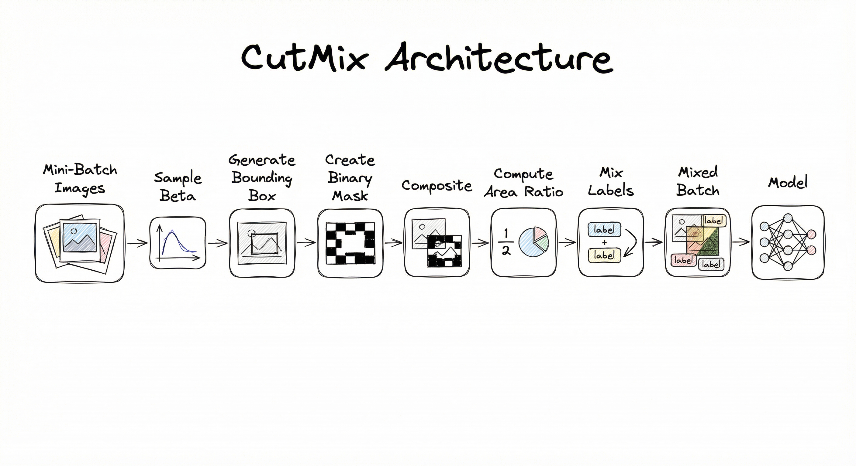
The Algorithm (Step by Step)
Let's build up the math from first principles. CutMix operates on pairs of training examples, so consider two images and drawn from the training set, where and is a one-hot label vector.
Step 1: Sample the mixing ratio.
Draw from a Beta distribution, where is a hyperparameter (typically ). This determines the area ratio of the crop.
Step 2: Determine the bounding box.
The rectangular region to be cut and pasted is sampled uniformly with the constraint that the ratio of the box area to the total image area equals :
The center of the box is sampled uniformly:
The box is clipped to image boundaries, so the actual area ratio may differ slightly from the target.
Step 3: Create the binary mask.
Define a binary mask where inside the bounding box and outside it.
Step 4: Combine the images.
where denotes element-wise multiplication. In plain English: pixels outside the box come from image A, pixels inside the box come from image B.
Step 5: Mix the labels.
The actual area ratio after clipping is computed as:
The mixed label is:
The Training Objective
The loss for a CutMix training step is:
where is the model and is the classification loss (typically cross-entropy).
Why for Width and Height?
This is a detail many explanations skip. We want the area of the box to equal . Since the box has width and height , and the aspect ratio is preserved (same proportions as the original image):
So taking the square root of for each dimension ensures the area is correct.
The Role of the Beta Distribution
The Beta(, ) distribution is symmetric around 0.5. When (the recommended default), it becomes the uniform distribution on , meaning the patch can be anywhere from tiny to nearly full-image size. For , values cluster around 0.5 (moderate mixing). For , values push toward 0 or 1 (either very small or very large patches).
In practice, works well across most benchmarks, making CutMix effectively hyperparameter-free beyond the decision of whether to enable it.
Warning: When the bounding box is clipped to image boundaries, the actual area ratio may differ from the sampled . Always compute the label mixing from the actual clipped area, not the sampled . Getting this wrong is a subtle bug that degrades performance.
Internal Architecture
CutMix is implemented as a batch-level augmentation that operates within the training data pipeline, after standard per-image augmentations (random crop, horizontal flip) but before normalization and model forward pass. The architecture consists of four logical stages: ratio sampling, bounding box generation, image compositing, and label mixing. Because CutMix requires pairing images from the same batch, it is typically implemented as a collate function or an in-batch transformation rather than a per-image transform.
Key Components
Ratio Sampler
Draws from Beta(, ) distribution. Controls the size of the cut region. With , the distribution is uniform over , allowing patches of any size. Higher concentrates patches around 50% area coverage.
Bounding Box Generator
Computes the width and height of the rectangular patch, samples a random center point, and clips the box to image boundaries. Returns the final bounding box coordinates.
Binary Mask Creator
Creates a binary mask where pixels inside the bounding box are 0 (will receive content from image B) and pixels outside are 1 (retain content from image A).
Image Compositor
Produces the mixed image using element-wise multiplication and addition. This is a simple tensor operation, making CutMix computationally cheap.
Label Mixer
Computes the actual area ratio from the clipped bounding box and produces the soft label . This is fed to the loss function alongside the mixed image.
Data Flow
Here's how CutMix integrates into a typical training loop:
Per-Image Stage (in data loader __getitem__): Each image goes through standard augmentations — random resized crop, horizontal flip, color jitter — independently.
Batch-Level Stage (in collate function or training loop): A mini-batch of augmented images is assembled. CutMix pairs each image with another (typically by random permutation of batch indices). For each pair, the ratio sampler draws , the bounding box generator creates the crop region, the compositor creates the mixed image, and the label mixer produces the soft target.
Forward Pass: The mixed batch is normalized and fed to the model. The loss is computed using the soft labels, typically as a weighted sum of cross-entropy losses for both original labels.
CutMix adds negligible computational overhead — the masking and compositing operations are simple tensor operations that take <1ms per batch on modern GPUs.
A linear flow from a mini-batch of images through Beta distribution sampling, bounding box generation, binary mask creation, image compositing (element-wise multiply and add), area ratio computation, label mixing, and finally the mixed batch being fed to the model for training.
How to Implement
Implementation Approaches
CutMix is straightforward to implement and can be done in three ways:
Option A: From scratch — Write the Beta sampling, bounding box generation, and compositing logic yourself. This takes about 30-40 lines of Python and is useful for understanding the algorithm deeply.
Option B: Via training libraries — Use timm's built-in Mixup/CutMix implementation (recommended for production), which handles CutMix + Mixup switching, per-batch vs per-element mixing, and correct label handling.
Option C: Via augmentation libraries — torchvision.transforms.v2 includes a CutMix transform as of PyTorch 2.0. Albumentations does not natively support CutMix since it operates at the per-image level, not batch level.
The critical implementation detail most people miss: CutMix operates at the batch level, not the per-image level. It needs to pair images within a mini-batch, so it cannot be implemented as a standard per-image transform in the data loader's __getitem__ method. Instead, it should be applied in the collate function, in a custom batch transform, or directly in the training loop.
Cost Considerations
CutMix adds virtually zero computational cost — the tensor operations (masking, addition) take <1ms per batch on any modern GPU. There is no memory overhead beyond one extra copy of the shuffled batch indices. In terms of cloud costs, enabling CutMix adds approximately $0 to your training bill. The only cost is the engineering time to implement and validate it, which should be under an hour using timm (~₹500-1,000 of engineer time in India, or effectively free).
import torch
import numpy as np


def rand_bbox(size, lam):
    """Generate a random bounding box for CutMix."""
    W = size[2]
    H = size[3]
    cut_rat = np.sqrt(1.0 - lam)
    cut_w = int(W * cut_rat)
    cut_h = int(H * cut_rat)

    # Uniform sampling of center
    cx = np.random.randint(W)
    cy = np.random.randint(H)

    # Clip to image boundaries
    bbx1 = np.clip(cx - cut_w // 2, 0, W)
    bby1 = np.clip(cy - cut_h // 2, 0, H)
    bbx2 = np.clip(cx + cut_w // 2, 0, W)
    bby2 = np.clip(cy + cut_h // 2, 0, H)

    return bbx1, bby1, bbx2, bby2


def cutmix_data(x, y, alpha=1.0):
    """Apply CutMix augmentation to a batch.

    Args:
        x: batch of images (N, C, H, W)
        y: batch of labels (N,) integer class indices
        alpha: Beta distribution parameter (default 1.0 = uniform)

    Returns:
        mixed_x, y_a, y_b, lam (actual area ratio after clipping)
    """
    lam = np.random.beta(alpha, alpha)
    batch_size = x.size(0)
    index = torch.randperm(batch_size).to(x.device)

    bbx1, bby1, bbx2, bby2 = rand_bbox(x.size(), lam)

    # Paste patch from shuffled image onto original
    x[:, :, bbx1:bbx2, bby1:bby2] = x[index, :, bbx1:bbx2, bby1:bby2]

    # Recompute lambda from actual clipped box area
    lam = 1 - ((bbx2 - bbx1) * (bby2 - bby1) / (x.size(-1) * x.size(-2)))

    y_a, y_b = y, y[index]
    return x, y_a, y_b, lam


def cutmix_criterion(criterion, pred, y_a, y_b, lam):
    """Compute CutMix loss as weighted combination."""
    return lam * criterion(pred, y_a) + (1 - lam) * criterion(pred, y_b)


# === Training loop integration ===
import torch.nn as nn

model = ...  # Your model
optimizer = ...  # Your optimizer
criterion = nn.CrossEntropyLoss()

for images, labels in train_loader:
    images, labels = images.cuda(), labels.cuda()

    # Apply CutMix with probability 0.5
    if np.random.random() < 0.5:
        images, labels_a, labels_b, lam = cutmix_data(images, labels, alpha=1.0)
        outputs = model(images)
        loss = cutmix_criterion(criterion, outputs, labels_a, labels_b, lam)
    else:
        outputs = model(images)
        loss = criterion(outputs, labels)

    optimizer.zero_grad()
    loss.backward()
    optimizer.step()
This is the canonical CutMix implementation following the original paper. Key details: (1) rand_bbox computes the box dimensions using to ensure the area ratio matches . (2) After clipping to boundaries, the actual is recomputed from the clipped box area — this is critical for correct label mixing. (3) Images are paired via random permutation of batch indices. (4) CutMix is applied with probability 0.5 per batch, alternating with standard training. In production, you'd typically alternate between CutMix and Mixup rather than CutMix and no augmentation.
import torch
from timm.data.mixup import Mixup
from timm.data import create_dataset, create_loader
import timm

# Create model
model = timm.create_model('resnet50', pretrained=True, num_classes=1000)
model.cuda()

# Configure CutMix + Mixup (timm's default recipe)
# Switches between CutMix and Mixup with 50% probability each
mixup_fn = Mixup(
    mixup_alpha=0.8,       # Mixup Beta distribution alpha
    cutmix_alpha=1.0,      # CutMix Beta distribution alpha
    cutmix_minmax=None,    # Optional: constrain CutMix patch size
    prob=1.0,              # Probability of applying either CutMix or Mixup
    switch_prob=0.5,       # Probability of switching to CutMix (vs Mixup)
    mode='batch',          # 'batch' or 'elem' (per-element mixing)
    label_smoothing=0.1,   # Optional label smoothing on top of mixing
    num_classes=1000,
)

# Training loop
criterion = torch.nn.CrossEntropyLoss()

for images, labels in train_loader:
    images, labels = images.cuda(), labels.cuda()

    # Apply CutMix/Mixup — returns mixed images and soft labels
    images, labels = mixup_fn(images, labels)

    outputs = model(images)
    loss = criterion(outputs, labels)  # labels are already soft

    loss.backward()
    optimizer.step()
    optimizer.zero_grad()
The timm library provides a production-ready Mixup class that handles CutMix and Mixup together, switching between them with configurable probability. This is the recommended approach for production training: it handles edge cases (label smoothing integration, per-element vs per-batch mixing), works with any model in the timm ecosystem, and follows the exact recipe that achieves state-of-the-art results. The switch_prob=0.5 means each batch has a 50/50 chance of CutMix vs Mixup, which is the default in most modern training recipes.
import torch
from torchvision.transforms import v2
from torchvision.datasets import ImageFolder
from torch.utils.data import DataLoader

# Standard per-image transforms
transform = v2.Compose([
    v2.RandomResizedCrop(224),
    v2.RandomHorizontalFlip(),
    v2.ToImage(),
    v2.ToDtype(torch.float32, scale=True),
    v2.Normalize(mean=[0.485, 0.456, 0.406], std=[0.229, 0.224, 0.225]),
])

# CutMix and Mixup as batch-level transforms
cutmix = v2.CutMix(num_classes=1000, alpha=1.0)
mixup = v2.MixUp(num_classes=1000, alpha=0.2)
cutmix_or_mixup = v2.RandomChoice([cutmix, mixup])

# Dataset and DataLoader
dataset = ImageFolder(root='path/to/imagenet/train', transform=transform)
train_loader = DataLoader(dataset, batch_size=256, shuffle=True, num_workers=8)

# Apply CutMix/MixUp in the training loop (batch-level)
for images, labels in train_loader:
    images, labels = cutmix_or_mixup(images, labels)
    # labels are now soft (N, num_classes)
    outputs = model(images)
    loss = criterion(outputs, labels)
    loss.backward()
    optimizer.step()
    optimizer.zero_grad()
PyTorch's torchvision.transforms.v2 provides native CutMix and MixUp transforms that operate at the batch level. v2.RandomChoice randomly selects one of CutMix or MixUp for each batch. Note that these transforms convert integer labels to one-hot soft labels automatically, so the loss function must accept soft targets (use nn.CrossEntropyLoss which handles this in modern PyTorch). This approach is cleaner than writing CutMix from scratch but less configurable than timm's implementation.
import torch
import numpy as np
from typing import List, Tuple


def cutmix_detection(
    image_a: torch.Tensor,
    boxes_a: torch.Tensor,
    labels_a: torch.Tensor,
    image_b: torch.Tensor,
    boxes_b: torch.Tensor,
    labels_b: torch.Tensor,
    alpha: float = 1.0,
) -> Tuple[torch.Tensor, torch.Tensor, torch.Tensor]:
    """CutMix for object detection — preserves bounding boxes.

    Args:
        image_a, image_b: (C, H, W) tensors
        boxes_a, boxes_b: (N, 4) tensors in xyxy format
        labels_a, labels_b: (N,) class label tensors
        alpha: Beta distribution parameter

    Returns:
        mixed_image, merged_boxes, merged_labels
    """
    _, H, W = image_a.shape
    lam = np.random.beta(alpha, alpha)

    # Generate bounding box for the cut region
    cut_w = int(W * np.sqrt(1 - lam))
    cut_h = int(H * np.sqrt(1 - lam))
    cx, cy = np.random.randint(W), np.random.randint(H)
    x1 = np.clip(cx - cut_w // 2, 0, W)
    y1 = np.clip(cy - cut_h // 2, 0, H)
    x2 = np.clip(cx + cut_w // 2, 0, W)
    y2 = np.clip(cy + cut_h // 2, 0, H)

    # Composite image
    mixed = image_a.clone()
    mixed[:, y1:y2, x1:x2] = image_b[:, y1:y2, x1:x2]

    # Keep boxes from image_a that are mostly outside the cut region
    keep_a = []
    for i, box in enumerate(boxes_a):
        bx1, by1, bx2, by2 = box.tolist()
        # Compute overlap with cut region
        inter_x1 = max(bx1, x1)
        inter_y1 = max(by1, y1)
        inter_x2 = min(bx2, x2)
        inter_y2 = min(by2, y2)
        inter_area = max(0, inter_x2 - inter_x1) * max(0, inter_y2 - inter_y1)
        box_area = (bx2 - bx1) * (by2 - by1)
        if box_area > 0 and inter_area / box_area < 0.5:  # Keep if <50% occluded
            keep_a.append(i)

    # Keep boxes from image_b that are mostly inside the cut region
    keep_b = []
    for i, box in enumerate(boxes_b):
        bx1, by1, bx2, by2 = box.tolist()
        # Clip box to cut region
        clipped = torch.tensor([max(bx1, x1), max(by1, y1), min(bx2, x2), min(by2, y2)])
        clipped_area = max(0, clipped[2] - clipped[0]) * max(0, clipped[3] - clipped[1])
        box_area = (bx2 - bx1) * (by2 - by1)
        if box_area > 0 and clipped_area / box_area > 0.5:  # Keep if >50% inside
            keep_b.append((i, clipped))

    # Merge boxes and labels
    merged_boxes = [boxes_a[i] for i in keep_a] + [b for _, b in keep_b]
    merged_labels_list = [labels_a[i] for i in keep_a] + [labels_b[i] for i, _ in keep_b]

    if merged_boxes:
        merged_boxes = torch.stack(merged_boxes)
        merged_labels = torch.stack(merged_labels_list)
    else:
        merged_boxes = torch.zeros((0, 4))
        merged_labels = torch.zeros((0,), dtype=torch.long)

    return mixed, merged_boxes, merged_labels
Extending CutMix to object detection requires careful handling of bounding boxes. This implementation preserves boxes from image A that are mostly outside the cut region (less than 50% occluded) and boxes from image B that are mostly inside the cut region (more than 50% visible). Boxes from image B are clipped to the cut region boundaries. This approach is used in YOLO training pipelines and the Ultralytics library. The 50% IoU threshold is configurable — stricter thresholds preserve fewer but more reliable annotations.
# timm CutMix/Mixup configuration (YAML)
augmentation:
  mixup_alpha: 0.8        # Beta(0.8, 0.8) for Mixup
  cutmix_alpha: 1.0       # Beta(1.0, 1.0) for CutMix (uniform)
  cutmix_minmax: null     # Optional: [0.2, 0.8] constrains patch size
  prob: 1.0               # Always apply one of CutMix/Mixup
  switch_prob: 0.5         # 50% chance of CutMix vs Mixup
  mode: batch              # 'batch' = same mix for all in batch
  label_smoothing: 0.1     # Additional label smoothing
  num_classes: 1000
Common Implementation Mistakes
- ●
Using sampled lambda instead of actual area ratio for label mixing: After clipping the bounding box to image boundaries, the actual area ratio changes. Using the original sampled instead of recomputing from the clipped box area produces incorrect soft labels. This is a silent bug — training still converges, but accuracy is lower than it should be.
- ●
Implementing CutMix as a per-image transform: CutMix requires pairing two images, so it must operate at the batch level (in the collate function or training loop). Implementing it in the dataset's
__getitem__method would require loading a second random image, which is possible but breaks data loader parallelism and cache efficiency. - ●
Applying CutMix after normalization: CutMix should be applied to unnormalized (or consistently normalized) images. If images are normalized with different statistics before mixing, the cut boundary will have visible artifacts, and the mixed image will have inconsistent pixel value distributions.
- ●
Not handling the edge case where the box has zero area: When is very close to 1.0, the box can be clipped to zero area, resulting in no mixing. The actual should be 1.0 in this case (pure image A). Some implementations don't handle this gracefully, dividing by zero when computing the area ratio.
- ●
Forgetting to switch to hard labels at validation time: CutMix produces soft labels during training, but validation should use standard hard labels with unaugmented images. Evaluating with CutMix-augmented validation images will give misleading metrics.
When Should You Use This?
Use When
You are training an image classification model and want a simple, near-free regularization boost — CutMix typically adds 0.5-2.5% top-1 accuracy with zero additional compute cost
Your task benefits from better localization (object detection, weakly-supervised localization, fine-grained recognition) — CutMix trains models to attend to all parts of objects, not just the most discriminative region
You have limited labeled data and need to extract maximum information from every training image — CutMix wastes no pixels, unlike Cutout which throws away information
You want to improve model calibration — CutMix's proportional label mixing trains models to produce well-calibrated confidence scores rather than overconfident hard predictions
You need improved robustness to occlusions and input corruptions — CutMix-trained models handle partial visibility better because they've seen occluded objects during training
You're using a modern training recipe (timm, torchvision v2) and want to match published state-of-the-art results — CutMix is a standard component in virtually all competitive training pipelines
Avoid When
Your task is pixel-precise and requires intact spatial structure throughout the image — e.g., dense stereo matching, image registration, or pixel-level correspondence where cutting and pasting would break geometric relationships
Labels are strictly position-dependent — e.g., action recognition where the spatial relationship between body parts is essential, or pose estimation where cutting creates anatomically impossible configurations
Your dataset has extremely high label noise (>15%) — CutMix compounds label noise because it combines labels from two potentially mislabeled images. Clean your labels first
You're working with very small images (e.g., 8x8 or 16x16 feature patches) where even a small cut region destroys most of the content, leaving insufficient signal for either class
Your images have critical text or sequential information that would be disrupted by cutting — e.g., OCR on document images where cutting would create unreadable text fragments
Training time is severely constrained and you need the simplest possible pipeline — while CutMix itself is cheap, debugging incorrect implementations can waste time. In this case, use a library (timm) or skip it
Key Tradeoffs
CutMix vs Mixup: When Does Each Win?
This is the question you'll face most often. The short answer: CutMix wins for localization-sensitive tasks; Mixup wins for smooth feature interpolation; combining both is usually best.
| Dimension | CutMix | Mixup |
|---|---|---|
| Spatial locality | Preserved (clean rectangular boundary) | Destroyed (global pixel blending) |
| Localization quality | Excellent (+5.4% over Mixup on CUB-200) | Poor (blurred spatial features) |
| Image naturalness | Semi-natural (collage effect) | Unnatural (ghostly overlay) |
| Classification accuracy | Strong (+2.28% on ImageNet ResNet-50) | Strong (+1.0% on ImageNet) |
| Calibration | Good (proportional labels) | Excellent (smoothest interpolation) |
| Implementation | Batch-level, slightly complex | Batch-level, very simple |
In practice, the CutMix + Mixup combination (switching between them randomly per batch with 50/50 probability) consistently outperforms either alone. This is the default in timm and is used in most state-of-the-art training recipes.
CutMix vs Cutout: A Clear Winner
CutMix strictly dominates Cutout in almost every scenario. Both occlude a rectangular region, but CutMix fills it with useful content (another training image) while Cutout fills it with zeros. CutMix achieves better accuracy, better localization, and better robustness, all at the same computational cost. Unless you specifically need the simplicity of Cutout (or your framework doesn't support batch-level augmentations), there is no reason to prefer Cutout over CutMix.
Cost Analysis
CutMix adds effectively zero cost:
- Compute: <1ms per batch of additional tensor operations. On an 8-GPU training run on ImageNet, this is ~$0 extra.
- Memory: One extra tensor for shuffled indices (negligible).
- Engineering time: ~1 hour if implementing from scratch, ~5 minutes if using
timm. At Indian rates, this is ₹500-5,000 of engineer time. - Accuracy gain: +0.5-2.5% top-1 on ImageNet-scale benchmarks, which can translate to meaningful improvements in production quality.
Rule of Thumb: Always enable CutMix (paired with Mixup, 50/50 switch probability) for image classification and detection training. The cost is zero and the benefit is consistent. The only question is whether to use (default, recommended) or tune it for your specific dataset.
Alternatives & Comparisons
Mixup blends entire images via convex combination (), creating ghostly overlays that destroy spatial locality. CutMix preserves spatial structure by operating on rectangular patches. CutMix generally outperforms Mixup for localization tasks (+5.4% on CUB-200 weakly-supervised localization) and classification (+0.6% on ImageNet). However, Mixup produces smoother feature interpolations and better calibration. Best practice: use both together, switching randomly per batch with 50/50 probability.
Standard augmentations (random crop, flip, color jitter, rotation) operate on single images and modify spatial or photometric properties. CutMix operates on image pairs and modifies content by pasting regions between images. CutMix is complementary to standard augmentations — you apply standard transforms first, then CutMix at the batch level. They serve different roles: standard augmentations encode invariances (rotation, scale, color), while CutMix provides regularization through occlusion and multi-object label mixing.
Random Erasing and Cutout mask out rectangular regions with random noise or zeros, forcing models to attend to multiple object parts. CutMix does the same but fills the region with useful content from another image, making every pixel count. CutMix strictly dominates Cutout on all benchmarks: +1.2% on ImageNet top-1, +5.4% on CUB-200 localization, and better corruption robustness. There is no scenario where Cutout is preferred over CutMix, assuming batch-level augmentation is feasible.
Pros, Cons & Tradeoffs
Advantages
Zero computational overhead — CutMix adds <1ms per batch of simple tensor masking and addition operations. No additional model forward passes, no extra data loading, no memory overhead beyond shuffled indices. It's as close to a free lunch as exists in deep learning.
Consistent accuracy improvement across architectures (ResNets, Vision Transformers, EfficientNets) and dataset scales (CIFAR-10 to ImageNet). Typical gains: +0.5-2.5% top-1 accuracy, which compound with other training recipe improvements.
Dramatically improves localization ability — CutMix-trained models produce higher-quality class activation maps (CAMs), with +5.4% weakly-supervised localization accuracy over Mixup on CUB-200. This transfers to detection and segmentation tasks where localization matters.
No wasted pixels — unlike Cutout which discards information by masking with zeros, CutMix fills every pixel with meaningful training signal from another image. This is especially valuable for small or low-resolution images where information density is critical.
Improves model robustness to input corruptions (noise, blur, weather effects) and improves out-of-distribution detection. Models trained with CutMix handle occluded and partially visible objects better in deployment.
Effectively hyperparameter-free — the default (uniform distribution for patch size) works well across virtually all benchmarks. No expensive hyperparameter search required, unlike AutoAugment.
Improves model calibration — proportional label mixing trains the model to output well-calibrated confidence scores rather than overconfident hard predictions, which is critical for safety-sensitive deployments (medical imaging, autonomous driving).
Disadvantages
Creates unnatural training images — the sharp rectangular boundary between two images is visually jarring and does not correspond to any natural image phenomenon. While models handle this well empirically, some purists argue it introduces a distributional artifact.
Requires batch-level implementation — unlike per-image augmentations, CutMix needs access to pairs of images, complicating data loading pipelines. It cannot be implemented as a standard transform in the dataset's
__getitem__method without workarounds.Label mixing may be inaccurate for non-uniform images — the area ratio assumes uniform semantic density across the image, which is often false. A CutMix patch that replaces the background of image A with the background of image B provides no additional class signal, yet the labels are still mixed. Saliency-aware variants (SaliencyMix, Puzzle Mix) address this at higher computational cost.
Less effective on very small images — on 32x32 images (CIFAR-10), CutMix patches are tiny and may not contain recognizable features, reducing the effectiveness of the method compared to larger-resolution datasets like ImageNet.
Compounds label noise — if the original labels have errors, CutMix mixes two potentially wrong labels, amplifying the noise. Datasets with >10% label noise may not benefit from CutMix without prior label cleaning.
Rectangular patches are a limitation — the fixed rectangular shape doesn't respect object boundaries. A CutMix patch might cut through the middle of an object, pasting half a cat ear next to half a dog ear. Non-rectangular variants (FMix, Puzzle Mix) address this but are more complex.
Failure Modes & Debugging
Area ratio mismatch from boundary clipping
Cause
When the randomly sampled bounding box center is near the image edge, clipping to image boundaries reduces the actual patch area. If the implementation uses the original sampled for label mixing instead of recomputing from the clipped area, the labels don't match the visual content.
Symptoms
Training converges but achieves 0.3-0.5% lower accuracy than expected. The discrepancy is subtle and hard to detect without comparing against a reference implementation. Label calibration metrics (ECE) are worse than expected because soft labels don't reflect actual content proportions.
Mitigation
Always recompute from the clipped bounding box area: lam = 1 - (bbx2 - bbx1) * (bby2 - bby1) / (W * H). Alternatively, use timm's implementation which handles this correctly. Add a unit test that verifies the returned matches the actual area ratio for edge-case bounding boxes.
CutMix applied during validation
Cause
Augmentation pipeline not properly disabled during validation/testing, causing CutMix to be applied to evaluation images. This is especially common when CutMix is implemented in the data loader collate function rather than conditionally in the training loop.
Symptoms
Validation accuracy is significantly lower than expected and fluctuates between runs (because CutMix introduces randomness). Validation loss is higher than training loss even when the model is not overfitting. Model appears to underperform compared to published baselines.
Mitigation
Conditionally apply CutMix only during training: if model.training:. If using a collate function, create separate collate functions for training and validation data loaders. Always verify that validation runs without CutMix by checking that validation accuracy matches expected baselines on a small test run.
Semantic mismatch with background-heavy images
Cause
CutMix mixes labels proportionally to the patch area, assuming semantic content is uniformly distributed. But many images have large backgrounds (sky, grass, water) and small foreground objects. A CutMix patch that replaces background in image A with background from image B changes the area ratio but adds zero class-relevant information, yet the label is still mixed.
Symptoms
Label noise increases for datasets with high background-to-foreground ratio (e.g., bird images where the bird occupies 10% of the image). Classification accuracy on such datasets improves less than expected. Fine-grained classification tasks may show degraded performance because subtle discriminative features are confused by irrelevant background mixing.
Mitigation
For fine-grained classification or background-heavy datasets, consider saliency-aware alternatives: SaliencyMix (uses saliency maps to select informative patches), SnapMix (uses CAMs for semantically proportional mixing), or Puzzle Mix (optimally transports salient regions). These add computational overhead but produce more accurate labels. Alternatively, use a smaller parameter (e.g., 0.3) to bias toward smaller patches that are more likely to hit the foreground object.
Incorrect loss function handling of soft labels
Cause
CutMix produces soft labels (probability distributions over classes), but some loss function implementations expect hard integer labels. Using nn.CrossEntropyLoss with integer targets and CutMix's soft labels causes a shape mismatch error or silent conversion to wrong values.
Symptoms
Runtime error about label shape mismatch (expected integer, got float tensor). Or training runs but produces poor accuracy because labels are incorrectly processed. In PyTorch, nn.CrossEntropyLoss actually handles both hard (integer) and soft (probability vector) labels as of recent versions, so the symptom may not manifest as an error but as subtle inaccuracy if using an older version.
Mitigation
Use the two-loss formulation: loss = lam * criterion(pred, y_a) + (1 - lam) * criterion(pred, y_b) where y_a and y_b are integer labels. This avoids converting to soft labels entirely. Alternatively, convert labels to one-hot vectors, mix them, and use nn.KLDivLoss or nn.BCEWithLogitsLoss which natively accept probability targets. If using timm, the Mixup class handles this automatically.
CutMix with batch size 1 or very small batches
Cause
CutMix pairs images within the same batch via random permutation. With batch size 1, the only pairing is the image with itself, producing no augmentation. With very small batches (2-4), pairing diversity is limited, reducing the regularization effect.
Symptoms
No accuracy improvement from CutMix (batch size 1). Minimal improvement with very small batches. Effective batch diversity is much lower than expected — the model sees the same image pairs repeatedly across epochs.
Mitigation
Use a batch size of at least 16 (ideally 32-256) when using CutMix to ensure diverse pairings. If hardware limits batch size (e.g., training on a single GPU with large images), use gradient accumulation for the optimizer but apply CutMix to each sub-batch independently. Alternatively, pre-compute CutMix pairs in the data loader by loading two images per sample (requires custom dataset implementation).
Degraded performance on medical imaging with anatomical orientation
Cause
CutMix patches transplant regions from one medical scan to another, creating anatomically impossible images (e.g., a patch of right-lung tissue appearing in the left-lung area, or cardiac structures from one patient appearing in another's scan). The proportional labels assume this content is valid training signal.
Symptoms
Model learns anatomically incorrect features. Classification accuracy on lateralized conditions (e.g., left vs right pleural effusion) degrades. Localization of anatomical structures becomes unreliable. Radiologists reviewing model explanations (saliency maps) flag anatomically impossible feature attributions.
Mitigation
For medical imaging, use CutMix with caution. Options: (1) Restrict the CutMix patch to small areas () so the overall image remains recognizable. (2) Only pair images of the same anatomical region and orientation (e.g., only mix left-lung images with other left-lung images). (3) Use intra-class CutMix (mix only images of the same class) to avoid creating mixed pathological/normal regions. (4) Consider domain-specific alternatives like CarveMix (for 3D volumes) that respect anatomical boundaries.
Placement in an ML System
Where Does CutMix Sit in the Pipeline?
CutMix occupies a very specific position in the training pipeline:
- Data Loading: Images are loaded from disk (JPEG/PNG) and decoded to tensors.
- Per-Image Augmentation: Standard transforms are applied independently to each image — random resized crop, horizontal flip, color jitter, etc.
- Batch Assembly: Images are collated into a mini-batch.
- CutMix (this block): Pairs of images within the batch are selected, rectangular patches are cut from one and pasted onto the other, labels are mixed proportionally.
- Normalization: Channel-wise mean subtraction and standard deviation division.
- Model Forward Pass: The mixed batch is fed to the model.
- Loss Computation: Loss is computed using the mixed soft labels.
CutMix must come after per-image augmentations (otherwise the cut region wouldn't benefit from augmentation) and before normalization (to avoid artifacts at the cut boundary from incompatible normalization statistics).
Interaction with Other Augmentations
CutMix is commonly combined with:
- Mixup: Alternate randomly per batch (50/50 probability). This is the standard recipe in
timm. - RandAugment/TrivialAugment: Applied per-image before CutMix at the batch level. These are complementary — RandAugment handles geometric/photometric variation, CutMix handles regularization through content mixing.
- Label smoothing: Applied on top of CutMix's soft labels for additional regularization. A common setting is label smoothing.
Key Insight: CutMix is not a replacement for standard augmentation — it's an additional layer that provides a different type of regularization (content mixing and label softening). The best results come from combining CutMix with standard augmentations and Mixup, each operating at different levels of the pipeline.
Pipeline Stage
Data Preprocessing / Training Pipeline
Upstream
- Data Loader
- Image Augmentation (standard transforms)
- Random Resized Crop
Downstream
- Normalization
- Model Forward Pass
- Loss Computation
Scaling Bottlenecks
CutMix itself is not a bottleneck — the tensor operations are trivially fast (<1ms per batch on any GPU). The real scaling considerations are:
-
Batch size requirements: CutMix needs reasonably large batches (>16 images) for diverse pairing. On large models (ViT-L, Swin-L) that fit only 4-8 images per GPU, you need multi-GPU training with large effective batch sizes to make CutMix useful.
-
Interaction with distributed training: In multi-GPU training, CutMix should be applied per-GPU batch (not globally across GPUs), because pairing images across GPUs would require expensive all-to-all communication. This means each GPU sees different CutMix pairings, which is actually beneficial for regularization diversity.
-
Memory for soft labels: With CutMix, labels change from integer class indices (N bytes per batch) to one-hot vectors (N × C floats per batch, where C is the number of classes). For ImageNet with 1000 classes and batch size 256, this is 256 × 1000 × 4 bytes = ~1 MB — negligible compared to image memory.
The honest answer: CutMix does not introduce scaling bottlenecks. If your training pipeline is slow, the problem is elsewhere (data loading, augmentation CPU overhead, model size).
Production Case Studies
CutMix was developed by researchers at NAVER Corp. (South Korea's largest internet company) and evaluated on their NSML (NAVER Smart Machine Learning) platform. The research team demonstrated CutMix's effectiveness across classification (ImageNet, CIFAR-10/100), weakly-supervised localization (CUB-200, ImageNet), and robustness benchmarks. CutMix-trained ResNet-50 achieved 78.6% top-1 accuracy on ImageNet (vs 76.3% baseline), and +5.4% localization accuracy over Mixup on CUB-200. The technique is now integrated into NAVER's production vision pipelines for search and commerce image understanding.
CutMix improved ResNet-50 ImageNet top-1 accuracy by +2.28%, outperformed both Mixup (+0.6%) and Cutout (+1.2%), and became the standard augmentation technique used across NAVER's computer vision products.
The "ResNet Strikes Back" paper demonstrated that modern training recipes — including CutMix paired with Mixup at 50/50 switching probability — can dramatically improve performance of classic architectures without changing the model. A vanilla ResNet-50 trained with the timm recipe (including CutMix, Mixup, RandAugment, label smoothing) achieved 80.4% top-1 on ImageNet, compared to the original 76.1%. This 4.3% gain came entirely from training recipe improvements. The timm library, used by thousands of researchers and companies worldwide, includes CutMix as a default training component.
ResNet-50 accuracy improved from 76.1% to 80.4% on ImageNet (+4.3%) purely through training recipe improvements including CutMix. The timm library has been downloaded over 50 million times and is the de facto standard for vision model training.
A MICCAI 2024 paper ("Cut to the Mix") investigated data augmentation strategies for organ segmentation with limited labeled data. Counterintuitively, CutMix — the simplest approach that does not try to preserve anatomical plausibility — outperformed more elaborate methods designed specifically for medical imaging (CarveMix, ObjectAug, Anatomix). CutMix improved average Dice score by +4.9 compared to the state-of-the-art nnU-Net without augmentation. The finding suggests that the regularization effect of CutMix's random mixing is more beneficial than domain-specific anatomical constraints when labeled data is scarce.
CutMix improved organ segmentation Dice score by +4.9 over baseline nnU-Net, outperforming all domain-specific augmentation methods tested. This challenges the assumption that medical imaging requires specialized augmentation strategies.
Original CutMix paper by Yun et al. (2019) from arXiv, presenting a regularization strategy that cuts and pastes image patches during training while mixing ground truth labels proportionally, widely adopted in Kaggle image classification competitions.
Consistently outperforms state-of-the-art augmentation on CIFAR and ImageNet classification; CutMix-pretrained ImageNet models show improved transfer learning performance on Pascal detection and MS-COCO captioning benchmarks.
Tooling & Ecosystem
The most comprehensive implementation of CutMix for training, integrated with 800+ model architectures. timm.data.mixup.Mixup handles CutMix + Mixup switching, per-batch/per-element modes, label smoothing integration, and correct soft label generation. Recommended for production training. Used in the "ResNet Strikes Back" recipe that achieved 80.4% ImageNet top-1 with ResNet-50.
PyTorch's official augmentation library includes v2.CutMix as a batch-level transform. Works with v2.RandomChoice to alternate between CutMix and MixUp. Tight integration with PyTorch data loaders and automatic one-hot label conversion. Simpler API than timm but less configurable.
The official PyTorch implementation by the CutMix authors at NAVER Clova AI. Includes training scripts for ImageNet and CIFAR, pretrained models, and the exact configuration used in the paper. Best for reproducing paper results or understanding the canonical implementation.
Official Keras example implementing CutMix for TensorFlow/Keras workflows. Includes a complete training pipeline with CutMix applied as a preprocessing function. Good starting point for TensorFlow-centric teams.
Ultralytics YOLOv8 includes CutMix as a built-in augmentation for object detection training (called "mosaic" augmentation, which is a CutMix variant that tiles four images). Enabled by default in the YOLO training pipeline with configurable probability.
A comprehensive benchmarking toolkit for mix-based augmentations including CutMix, Mixup, SaliencyMix, FMix, Puzzle Mix, GridMix, ResizeMix, and 20+ other variants. Useful for comparing CutMix against alternatives and running ablation studies.
Research & References
Yun, S., Han, D., Oh, S.J., Chun, S., Choe, J., Yoo, Y. (2019)ICCV 2019 (Oral)
The original CutMix paper. Proposed cutting rectangular patches from one training image and pasting them onto another, mixing labels proportionally to area. Achieved +2.28% top-1 on ImageNet ResNet-50, +5.4% weakly-supervised localization over Mixup on CUB-200, and improved corruption robustness. Established CutMix as a standard training technique.
Zhang, H., Cisse, M., Dauphin, Y.N., Lopez-Paz, D. (2018)ICLR 2018
Introduced Mixup, the predecessor to CutMix. Trains on convex combinations of image pairs and their labels (). Improved generalization, calibration, and adversarial robustness. CutMix builds on Mixup by replacing global blending with localized patch pasting to preserve spatial structure.
DeVries, T., Taylor, G.W. (2017)arXiv preprint
Introduced Cutout (regional dropout), masking out random rectangular regions with zeros to improve regularization. Achieved 2.56% error on CIFAR-10 and 15.20% on CIFAR-100. CutMix was directly motivated by Cutout's limitation of wasting information in masked regions.
Wightman, R., Touvron, H., Jegou, H. (2021)NeurIPS 2021 Workshop
Demonstrated that modern training recipes (including CutMix + Mixup) can improve ResNet-50 from 76.1% to 80.4% top-1 on ImageNet — a 4.3% gain without architecture changes. Established CutMix + Mixup (50/50 switching) as the standard augmentation recipe in the timm library.
Kim, J.H., Choo, W., Song, H.O. (2020)ICML 2020
Proposed Puzzle Mix, which uses saliency information to optimally transport informative patches between images. Addresses CutMix's limitation of random patch placement (which may hit uninformative regions). Achieves state-of-the-art results but at higher computational cost than CutMix.
Harris, E., Marber, A., Sherr, N., Sherr, D. (2020)arXiv preprint
Proposed FMix, which uses random binary masks from Fourier space instead of CutMix's rectangular masks. Produces non-rectangular mixing regions that better respect object boundaries. Improves over CutMix on CIFAR-10 without additional training time.
Li, S., Liu, Z., Di, K., Xue, F., Liu, Z. (2024)arXiv preprint
Comprehensive survey covering 60+ mix-based augmentation methods including CutMix, Mixup, SaliencyMix, FMix, Puzzle Mix, and their variants. Provides systematic comparison across benchmarks, tasks, and domains. Positions CutMix as the foundational method that spawned an entire subfield.
Interview & Evaluation Perspective
Common Interview Questions
- ●
What is CutMix and how does it differ from Mixup and Cutout?
- ●
Explain the CutMix algorithm step by step. Why do you use the square root of (1 - lambda) for the box dimensions?
- ●
How does CutMix improve weakly-supervised object localization? Why does Mixup fail at this?
- ●
What is the role of the Beta distribution in CutMix? What happens with different alpha values?
- ●
When would you NOT use CutMix? Give specific examples.
- ●
How would you implement CutMix for object detection? What additional considerations are needed?
- ●
Explain how CutMix labels are computed. What happens when the bounding box is clipped to image boundaries?
- ●
You're training a medical imaging classifier. Should you use CutMix? What modifications would you make?
- ●
Compare CutMix with saliency-aware alternatives like Puzzle Mix and SaliencyMix. When is the extra complexity worth it?
Key Points to Mention
- ●
CutMix combines the benefits of Cutout (regularization through occlusion) and Mixup (using all training signal) while avoiding their weaknesses (information waste and spatial locality destruction, respectively). Lead with this framing.
- ●
Labels are mixed proportionally to the actual clipped area ratio, not the sampled lambda. This is a critical implementation detail that many people get wrong and that interviewers love to probe.
- ●
CutMix dramatically improves weakly-supervised localization (+5.4% over Mixup on CUB-200) because it forces the model to recognize objects from partial views in specific spatial regions, producing better class activation maps (CAMs).
- ●
The Beta(1.0, 1.0) distribution is uniform on [0, 1], meaning patch sizes range from tiny to full-image. This default works across virtually all benchmarks — CutMix is effectively hyperparameter-free.
- ●
In production, CutMix is almost always paired with Mixup (50/50 switching per batch). This is the default in timm and was used in the 'ResNet Strikes Back' recipe that improved ResNet-50 from 76.1% to 80.4% on ImageNet.
- ●
For object detection, CutMix requires additional handling of bounding boxes — you must decide which boxes to keep based on their overlap with the cut region. The standard threshold is 50% IoU.
Pitfalls to Avoid
- ●
Saying CutMix and Mixup are interchangeable — they have fundamentally different effects on spatial locality. CutMix preserves it, Mixup destroys it. This matters for localization-sensitive tasks.
- ●
Forgetting that CutMix is a batch-level operation, not a per-image transform. It requires image pairs from the same batch.
- ●
Not mentioning the boundary clipping issue: when the box center is near the image edge, the clipped area differs from the target area, and labels must be recomputed. This is the most common implementation bug.
- ●
Claiming CutMix works for all domains — it can be problematic for medical imaging (anatomical orientation matters), text/document images (cutting disrupts readability), and extremely small images (patches too small to be informative).
- ●
Ignoring saliency-aware alternatives when discussing CutMix's limitations. A senior candidate should know about Puzzle Mix, SaliencyMix, and FMix as extensions that address CutMix's random patch placement.
Senior-Level Expectation
A senior candidate should discuss CutMix in the context of a complete training recipe — not in isolation. This means explaining how it interacts with Mixup (50/50 switching), RandAugment (applied per-image before CutMix at batch level), label smoothing (applied on top of CutMix soft labels), and loss function choice (binary cross-entropy vs cross-entropy for soft targets). They should know the timm implementation and the "ResNet Strikes Back" recipe that achieved 80.4% with a vanilla ResNet-50. They should articulate CutMix's specific advantage over Mixup for localization tasks (spatial locality preservation) and its limitation of uniform semantic density assumption (saliency-aware alternatives). For medical imaging or specialized domains, they should discuss modifications (intra-class CutMix, small alpha, restricted pairing) rather than blindly applying the default recipe. Cost-wise, they should note that CutMix is computationally free — the decision is whether to implement it from scratch (₹500-5,000 of engineering time) or use timm (₹0, 5 minutes of configuration). At Indian ML startups, this kind of cost-awareness separates senior from mid-level engineers.
Summary
Let's recap what we've covered about CutMix:
-
CutMix is a mixed-sample data augmentation technique that cuts a rectangular patch from one training image and pastes it onto another, mixing their labels proportionally to the patch area. It was introduced by Yun et al. at ICCV 2019 and has become a standard component in virtually all state-of-the-art vision training recipes.
-
CutMix addresses the limitations of two predecessors: Cutout (which wastes information by masking with zeros) and Mixup (which destroys spatial locality by blending entire images). By filling the masked region with content from another image, CutMix uses every pixel for training while preserving clear spatial boundaries between classes. This is why it outperforms both: +2.28% over baseline, +1.2% over Cutout, and +0.6% over Mixup on ImageNet top-1 accuracy.
-
The algorithm is simple: sample a mixing ratio from Beta(, ), compute box dimensions using , randomly place the box, paste the patch, and mix labels proportionally to the actual clipped area. With (uniform distribution), CutMix is effectively hyperparameter-free.
-
CutMix's most distinctive advantage is dramatically improved localization (+5.4% over Mixup on CUB-200 weakly-supervised localization). By occluding parts of objects with content from other images, CutMix forces models to attend to all discriminative regions, producing higher-quality class activation maps.
-
In production, CutMix is paired with Mixup (50/50 switching per batch), combined with RandAugment and label smoothing. The
timmlibrary's default recipe — which includes CutMix — improved ResNet-50 from 76.1% to 80.4% on ImageNet without architecture changes.
CutMix is one of the highest-ROI techniques in modern deep learning: zero computational cost, minimal implementation effort, and consistent accuracy and localization improvements across architectures and datasets. If you're training an image classifier in 2026 and not using CutMix, you're leaving free performance on the table.