Borderline-SMOTE in Machine Learning
Vanilla SMOTE treats every minority sample identically — whether it sits safely in the heart of a minority cluster or teeters right on the edge of the decision boundary. That egalitarian approach sounds fair, but it wastes synthetic samples on regions where the classifier already has the picture figured out, while under-investing in the contested borderland where classification actually happens.
Borderline-SMOTE, introduced by Han, Wang, and Mao in 2005, fixes this by asking a simple but powerful question: which minority samples actually need help? The answer turns out to be the ones living in the DANGER zone — minority instances whose k-nearest neighbors include a significant proportion of majority class samples. These are the samples the classifier struggles with, and they are precisely where targeted synthetic oversampling yields the highest marginal return.
The algorithm partitions every minority sample into one of three groups — SAFE, DANGER, or NOISE — based on neighborhood composition, then generates synthetic samples exclusively from the DANGER set. This focused strategy concentrates the synthetic budget on the decision boundary, sharpening the classifier's ability to distinguish classes exactly where it matters most. Two variants, Borderline-1 and Borderline-2, offer different interpolation strategies for even finer control.
Today, Borderline-SMOTE is a first-line resampling method in production ML systems at companies ranging from Indian fintech firms detecting UPI fraud to global healthcare platforms triaging rare diseases. It is available out of the box in imbalanced-learn as BorderlineSMOTE, making adoption trivial for any Python ML pipeline.
Concept Snapshot
- What It Is
- A selective oversampling technique that generates synthetic minority class samples exclusively for instances near the decision boundary (DANGER set), rather than uniformly across all minority samples.
- Category
- Data Generation
- Complexity
- Intermediate
- Inputs / Outputs
- Inputs: imbalanced training dataset with minority and majority classes. Outputs: balanced dataset with synthetic minority samples generated only from borderline (DANGER) instances.
- System Placement
- Applied during data preprocessing, after data cleaning, feature scaling, and train-test split, but before model training or cross-validation.
- Also Known As
- BSMOTE, Borderline Synthetic Minority Over-sampling, BLSMOTE, Boundary-focused SMOTE
- Typical Users
- ML engineers, data scientists, research scientists, fraud analytics teams, medical AI researchers
- Prerequisites
- SMOTE algorithm fundamentals, k-nearest neighbors, class imbalance and decision boundaries, Euclidean distance and feature scaling, precision-recall tradeoffs
- Key Terms
- DANGER setSAFE setNOISE setm_neighborsk_neighborsborderline-1borderline-2decision boundaryneighborhood composition
Why This Concept Exists
The Problem with Uniform Oversampling
Vanilla SMOTE generates synthetic minority samples by uniformly selecting from all minority instances and interpolating between them and their k-nearest neighbors. This means a minority sample buried deep inside a homogeneous minority cluster — far from any majority sample — receives the same oversampling treatment as a minority sample surrounded by majority class neighbors on the brink of misclassification.
The result is predictable: synthetic samples pile up in safe, interior regions where the classifier already performs well, while the contested decision boundary remains underserved. Empirical studies have shown that 40-60% of SMOTE-generated synthetic samples fall in regions that contribute little to improving the classifier's discrimination ability.
The Decision Boundary Insight
Classification performance is determined almost entirely at the decision boundary — the region in feature space where the classifier transitions from predicting one class to predicting another. Minority samples near this boundary are the ones the model struggles with and the ones that influence the boundary's shape. Supporting these borderline cases with additional synthetic examples is far more valuable than padding interior clusters.
Han, Wang, and Mao formalized this insight in their 2005 paper at the International Conference on Intelligent Computing (ICIC). They observed that minority samples can be partitioned into three groups based on the composition of their local neighborhood:
- SAFE: Mostly surrounded by other minority samples — the classifier handles these well.
- DANGER: Surrounded by a mix of minority and majority samples — these are the contested borderline cases.
- NOISE: Surrounded almost entirely by majority samples — likely outliers or mislabeled instances.
By generating synthetic samples only from the DANGER set, Borderline-SMOTE concentrates its oversampling budget exactly where the classifier needs the most help.
Why This Matters in Practice
Consider fraud detection at an Indian digital payments company processing 10 million UPI transactions daily. Out of every 100,000 transactions, perhaps 50 are fraudulent (0.05% minority rate). Some fraudulent patterns — say, suspicious midnight international transfers — are unmistakable; the classifier catches them easily. But borderline cases — a legitimate-looking ₹4,999 transfer (just under the ₹5,000 threshold that triggers extra verification) from a device that matches the user's usual pattern but targets a new beneficiary — are where fraud slips through.
Vanilla SMOTE would waste synthetic samples reinforcing the easy-to-catch patterns. Borderline-SMOTE focuses its firepower on these ambiguous, boundary-straddling cases, teaching the model to make sharper distinctions where they matter most.
Historical Context: Borderline-SMOTE (2005) was one of the first principled modifications to the original SMOTE algorithm (Chawla et al., 2002). It predates ADASYN (He et al., 2008) by three years and introduced the concept of neighborhood-based sample categorization that influenced many subsequent SMOTE variants including Safe-Level SMOTE, LN-SMOTE, and cluster-based SMOTE.
Core Intuition & Mental Model
The Triage Analogy
Imagine you're managing a hospital emergency department during a crisis. You have limited resources (synthetic samples) and three groups of patients:
-
Stable patients (SAFE set): Already recovering, don't need immediate intervention. These are minority samples deep inside their own cluster — the classifier handles them fine.
-
Critical patients (DANGER set): In the danger zone, could go either way. These are minority samples near the decision boundary, surrounded by a mix of minority and majority neighbors. They desperately need attention.
-
Terminal patients (NOISE set): Isolated outliers so deep in enemy territory that intervening is likely futile and may even cause harm. These are minority samples completely surrounded by majority class samples — probably mislabeled or extreme anomalies.
A smart triage system directs all resources to Group 2. That's exactly what Borderline-SMOTE does.
The Geometric Picture
Visualize a 2D feature space. Minority samples (red dots) cluster in one region, majority samples (blue dots) in another, with a contested border zone where the two populations intermingle.
Vanilla SMOTE would scatter synthetic red dots throughout the entire red region — including deep inside where blue dots never appear. Borderline-SMOTE instead identifies red dots that have blue neighbors (the DANGER set) and generates new synthetic red dots only near these contested locations.
The effect is like reinforcing a military front line: you don't station troops in the capital far from the border — you station them at the frontier where the action is.
Why Ignoring NOISE Samples Is Crucial
Here's an insight that trips up many practitioners: NOISE samples are not just low-value — they're actively harmful. A minority sample completely surrounded by majority neighbors is likely an outlier, mislabeled point, or extremely rare edge case. Generating synthetic samples around it would scatter minority-labeled points deep into majority territory, confusing the classifier and degrading precision.
By explicitly excluding NOISE samples from synthetic generation, Borderline-SMOTE avoids the noise amplification problem that plagues vanilla SMOTE on dirty datasets. This makes it inherently more robust to label noise and outliers.
Expert Insight: The ratio of SAFE:DANGER:NOISE samples in your minority class is itself a diagnostic signal. If >50% are NOISE, your minority class likely has severe label quality issues. If >80% are SAFE, your classes are well-separated and you might not need oversampling at all. A healthy ratio for Borderline-SMOTE is 30-50% DANGER, indicating a genuine decision boundary challenge.
Technical Foundations
Mathematical Formulation
Let be a training set with binary labels , where class 1 is the minority class with samples and class 0 is the majority class with samples, and .
Step 1: Neighborhood-Based Categorization
For each minority sample (where ), compute its nearest neighbors from the entire dataset (both classes). Let be the number of majority class samples among these neighbors.
Categorize as:
The DANGER set contains the borderline minority samples.
Step 2: Synthetic Sample Generation (Borderline-1)
For each :
- Find nearest neighbors of among minority class samples only
- Randomly select one neighbor from these minority neighbors
- Generate a synthetic sample:
Step 3: Synthetic Sample Generation (Borderline-2)
Borderline-2 extends Borderline-1 by also interpolating with majority class neighbors. For each :
- Find nearest neighbors of among all samples (both classes)
- If the selected neighbor belongs to the minority class, use the standard formula with
- If the selected neighbor belongs to the majority class, use a restricted range:
The restricted ensures the synthetic sample stays closer to the minority sample rather than drifting into majority territory.
Key Parameters
- (m_neighbors): Number of nearest neighbors from the full dataset used to classify each minority sample as SAFE/DANGER/NOISE. Default: 10 in imbalanced-learn.
- (k_neighbors): Number of nearest minority-class neighbors used for synthetic sample interpolation. Default: 5.
- kind: Choice of Borderline-1 (interpolate only with minority neighbors) or Borderline-2 (also interpolate with majority neighbors).
Computational Complexity
- Categorization step: for computing nearest neighbors from the full dataset of samples with features
- Synthetic generation: for k-NN search within minority class
- Total:
With ball tree or KD-tree acceleration, this reduces to for the categorization step.
Mathematical Note: The DANGER set condition means that at least half of a minority sample's neighbors must be from the majority class for it to be considered borderline. Setting too small (e.g., ) makes this categorization unstable; setting it too large (e.g., ) over-smooths local structure. The default provides a robust compromise for most datasets.
Internal Architecture
Borderline-SMOTE extends vanilla SMOTE with an additional categorization layer that partitions minority samples before synthetic generation. The architecture has two main phases: a classification phase that labels each minority sample as SAFE, DANGER, or NOISE using full-dataset k-NN, and a generation phase that applies standard SMOTE interpolation exclusively to DANGER samples.
The two-phase design means Borderline-SMOTE is slightly more expensive than vanilla SMOTE — it requires an extra k-NN pass over the full dataset — but the focused generation typically produces higher-quality synthetic samples that improve classifier performance at the decision boundary.
Key Components
Minority Class Extractor
Identifies all samples belonging to the minority class from the training set. In multi-class settings, applies a one-vs-rest decomposition to handle each class pair independently.
Full-Dataset m-NN Classifier
For each minority sample, finds its nearest neighbors from the entire dataset (both minority and majority classes). This is the categorization step that distinguishes Borderline-SMOTE from vanilla SMOTE. Uses Euclidean distance by default; implementations support alternative metrics.
SAFE/DANGER/NOISE Partitioner
Counts the number of majority-class neighbors among each minority sample's nearest neighbors and assigns the sample to SAFE (), DANGER (), or NOISE (). Only DANGER samples proceed to synthetic generation.
Minority-Class k-NN Finder
For each DANGER sample, finds its nearest neighbors within the minority class only. These intra-class neighbors serve as interpolation partners for synthetic sample generation. This is the same k-NN step used in vanilla SMOTE, but applied only to the DANGER subset.
Interpolation Engine (Borderline-1 / Borderline-2)
Generates synthetic samples by linear interpolation. Borderline-1: interpolates between the DANGER sample and a randomly selected minority neighbor with . Borderline-2: can also interpolate with majority neighbors using a restricted to keep synthetics closer to the minority sample.
Dataset Combiner
Merges original majority samples, original minority samples (SAFE + DANGER + NOISE, all preserved), and newly generated synthetic minority samples into the final balanced training set.
Data Flow
Input Flow: The algorithm receives the imbalanced training dataset and target sampling_strategy. It first separates minority class samples from the rest of the dataset.
Categorization Flow: Each minority sample undergoes m-nearest-neighbor lookup against the full dataset. Based on the fraction of majority neighbors, it is labeled SAFE, DANGER, or NOISE. Only DANGER samples are flagged for synthetic generation. The categorization results — particularly the indices of DANGER samples — are stored as metadata (accessible via the danger_indices_ attribute in imbalanced-learn).
Generation Flow: For each DANGER sample, the algorithm performs a second k-NN search, this time restricted to minority class samples only. It selects neighbors from this intra-class neighborhood and generates synthetic samples via linear interpolation. In Borderline-1, all interpolation partners are minority samples. In Borderline-2, majority class neighbors may also be used with a restricted interpolation range.
Output Flow: All original samples (SAFE, DANGER, NOISE, and majority) are preserved in the output. The newly generated synthetic minority samples are appended, producing a dataset where the minority class has been augmented to match the target sampling ratio. Critically, the NOISE samples are not removed — they remain in the dataset but do not spawn synthetic children.
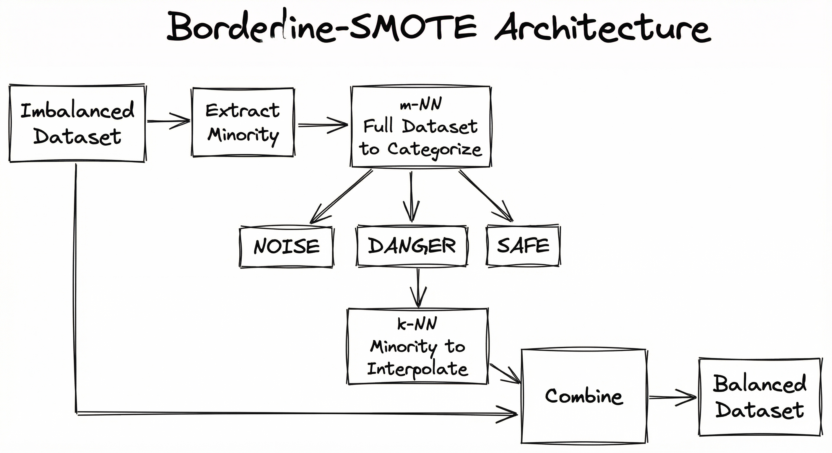
A flowchart showing the Borderline-SMOTE pipeline: starting from an imbalanced dataset, extracting minority samples, performing m-NN classification against the full dataset, partitioning into NOISE (excluded from generation), DANGER (selected for generation), and SAFE (excluded from generation), then performing k-NN within the minority class for DANGER samples, generating synthetic samples via interpolation, and combining everything into a balanced dataset.
How to Implement
Implementation Approaches
Borderline-SMOTE is implemented in the imbalanced-learn library as BorderlineSMOTE, following the same fit_resample() API as all other imblearn resamplers. The key configuration decisions are:
-
m_neighbors(default 10): Controls the categorization sensitivity. Higher values produce more stable SAFE/DANGER/NOISE assignments but may over-smooth local structure. Lower values are more responsive to local neighborhood composition but noisier. -
k_neighbors(default 5): Controls the interpolation neighborhood for synthetic generation, identical to vanilla SMOTE'skparameter. -
kind('borderline-1' or 'borderline-2'): Borderline-1 interpolates only with minority neighbors (conservative). Borderline-2 also interpolates with majority neighbors using a restricted range (more aggressive, pushes synthetics closer to the boundary).
For production systems, Borderline-SMOTE should be integrated via imblearn.pipeline.Pipeline to ensure correct cross-validation behavior. The algorithm is training-time only — no synthetic samples are generated at inference.
Performance characteristics: Borderline-SMOTE is slightly slower than vanilla SMOTE due to the extra m-NN categorization pass over the full dataset. For a dataset with 100,000 total samples and 1,000 minority samples, expect the categorization step to add 2-5 seconds on a modern CPU. The generation step is typically faster than vanilla SMOTE because only DANGER samples (usually 30-60% of minority samples) participate in synthetic generation.
Cost Note: Running Borderline-SMOTE on a dataset with 1M total samples on an AWS c6i.4xlarge (16 vCPUs, ~$0.68/hr or ~₹57/hr) takes approximately 3-8 minutes including both categorization and generation phases. For larger datasets, consider approximate nearest neighbor libraries or partial balancing.
from imblearn.over_sampling import BorderlineSMOTE
from sklearn.datasets import make_classification
from sklearn.model_selection import train_test_split
from sklearn.ensemble import RandomForestClassifier
from sklearn.metrics import classification_report
import numpy as np

# Create imbalanced dataset (1:50 ratio)
X, y = make_classification(
    n_classes=2,
    weights=[0.02, 0.98],
    n_samples=10000,
    n_features=20,
    n_informative=15,
    n_clusters_per_class=2,
    random_state=42
)

print(f"Original class distribution: {np.bincount(y)}")
# Output: [200, 9800]

# Train-test split FIRST
X_train, X_test, y_train, y_test = train_test_split(
    X, y, test_size=0.2, random_state=42, stratify=y
)

# Apply Borderline-SMOTE to training data only
bsmote = BorderlineSMOTE(
    sampling_strategy='auto',
    k_neighbors=5,
    m_neighbors=10,
    kind='borderline-1',
    random_state=42
)
X_train_res, y_train_res = bsmote.fit_resample(X_train, y_train)

print(f"Resampled class distribution: {np.bincount(y_train_res)}")
# Output: [7840, 7840] — balanced via DANGER-focused generation

# Train on balanced data, evaluate on original distribution
clf = RandomForestClassifier(n_estimators=100, random_state=42)
clf.fit(X_train_res, y_train_res)

y_pred = clf.predict(X_test)
print(classification_report(y_test, y_pred))
This example demonstrates the standard Borderline-SMOTE workflow. Key points: (1) Always split data before applying resampling — never apply Borderline-SMOTE to the test set. (2) m_neighbors=10 controls the SAFE/DANGER/NOISE categorization. (3) kind='borderline-1' uses only minority-class neighbors for interpolation, which is the more conservative and commonly used variant. (4) The test set retains the original imbalanced distribution to reflect real-world performance.
from imblearn.over_sampling import BorderlineSMOTE
from sklearn.datasets import make_classification
from sklearn.model_selection import cross_val_score
from sklearn.svm import SVC
from imblearn.pipeline import Pipeline
import numpy as np

# Create dataset with overlapping classes
X, y = make_classification(
    n_classes=2,
    weights=[0.05, 0.95],
    n_samples=5000,
    n_features=10,
    n_informative=8,
    flip_y=0.05,  # 5% label noise
    class_sep=0.8,
    random_state=42
)

results = {}

for kind in ['borderline-1', 'borderline-2']:
    pipeline = Pipeline([
        ('bsmote', BorderlineSMOTE(
            sampling_strategy='auto',
            k_neighbors=5,
            m_neighbors=10,
            kind=kind,
            random_state=42
        )),
        ('classifier', SVC(kernel='rbf', gamma='scale', random_state=42))
    ])

    scores = cross_val_score(
        pipeline, X, y,
        cv=5,
        scoring='f1',
        n_jobs=-1
    )
    results[kind] = scores
    print(f"{kind}: F1 = {scores.mean():.3f} +/- {scores.std():.3f}")

# Typical output:
# borderline-1: F1 = 0.724 +/- 0.031
# borderline-2: F1 = 0.741 +/- 0.028
# Borderline-2 often wins with overlapping classes and SVMs
Borderline-2 generates synthetic samples by also interpolating with majority class neighbors (using a restricted lambda range of [0, 0.5]), which pushes synthetics closer to the boundary. This is particularly effective with SVM classifiers that need support vectors near the boundary. However, Borderline-2 introduces a slight risk of generating synthetics that are too close to majority samples, so it requires careful tuning of m_neighbors.
from imblearn.over_sampling import BorderlineSMOTE
import numpy as np

# Create dataset
np.random.seed(42)
n_majority = 5000
n_minority = 200

# Minority samples: some safe (clustered), some borderline, some noise
X_majority = np.random.randn(n_majority, 5)
X_minority_safe = np.random.randn(80, 5) + np.array([4, 4, 4, 4, 4])
X_minority_danger = np.random.randn(100, 5) + np.array([1, 1, 1, 1, 1])
X_minority_noise = np.random.randn(20, 5)  # Mixed in with majority

X = np.vstack([X_majority, X_minority_safe, X_minority_danger, X_minority_noise])
y = np.array([0]*n_majority + [1]*n_minority)

# Fit Borderline-SMOTE
bsmote = BorderlineSMOTE(
    sampling_strategy='auto',
    k_neighbors=5,
    m_neighbors=10,
    kind='borderline-1',
    random_state=42
)
X_res, y_res = bsmote.fit_resample(X, y)

# Diagnostic: How many synthetics were generated?
n_synthetic = np.sum(y_res == 1) - np.sum(y == 1)
print(f"Original minority samples: {np.sum(y == 1)}")
print(f"Synthetic samples generated: {n_synthetic}")
print(f"Total minority after resampling: {np.sum(y_res == 1)}")
print(f"")
print(f"DANGER set diagnostic:")
print(f"  If n_synthetic is much less than expected,")
print(f"  many minority samples were classified as SAFE or NOISE.")
print(f"  This means you may not need oversampling at all (mostly SAFE)")
print(f"  or your minority class has severe noise issues (mostly NOISE).")
This diagnostic example helps you understand how your minority class is being partitioned. If the DANGER set is very small (most samples are SAFE), your classes are well-separated and Borderline-SMOTE may not add much value. If many samples are NOISE, you have a data quality problem that should be addressed before resampling. A healthy DANGER set is typically 30-60% of the minority class.
from imblearn.pipeline import Pipeline
from imblearn.over_sampling import BorderlineSMOTE
from sklearn.preprocessing import StandardScaler
from sklearn.ensemble import GradientBoostingClassifier
from sklearn.model_selection import (
    cross_val_score,
    StratifiedKFold
)
from sklearn.metrics import make_scorer, f1_score, recall_score
import numpy as np

# Simulated fraud detection dataset
np.random.seed(42)
X = np.random.randn(50000, 25)
y = np.array([0]*49750 + [1]*250)  # 0.5% fraud rate

# Production pipeline: Scale -> Borderline-SMOTE -> Classify
pipeline = Pipeline([
    ('scaler', StandardScaler()),
    ('bsmote', BorderlineSMOTE(
        sampling_strategy=0.3,   # Target 30% ratio, not full 1:1
        k_neighbors=5,
        m_neighbors=10,
        kind='borderline-1',
        random_state=42
    )),
    ('classifier', GradientBoostingClassifier(
        n_estimators=200,
        max_depth=5,
        learning_rate=0.1,
        random_state=42
    ))
])

# Stratified CV ensures each fold has proportional minority samples
cv = StratifiedKFold(n_splits=5, shuffle=True, random_state=42)

# Evaluate on multiple metrics
for metric_name, scorer in [
    ('F1', make_scorer(f1_score)),
    ('Recall', make_scorer(recall_score)),
]:
    scores = cross_val_score(
        pipeline, X, y,
        cv=cv,
        scoring=scorer,
        n_jobs=-1
    )
    print(f"{metric_name}: {scores.mean():.3f} +/- {scores.std():.3f}")

# Note: sampling_strategy=0.3 is often better than 'auto' (1:1)
# for extreme imbalance — full balancing can overwhelm the classifier
# with synthetic samples and degrade precision.
This production-ready pipeline demonstrates three best practices: (1) Feature scaling before Borderline-SMOTE, since k-NN is distance-sensitive. (2) Partial balancing (sampling_strategy=0.3) instead of full 1:1, which often performs better for extreme imbalance. (3) Using imblearn.pipeline.Pipeline with StratifiedKFold to ensure SMOTE is applied correctly inside each cross-validation fold, preventing data leakage.
# Borderline-SMOTE configuration for imbalanced-learn

# Standard Borderline-1 configuration (recommended default)
borderline1_config = {
    'sampling_strategy': 'auto',   # Balance to 1:1
    'k_neighbors': 5,              # Interpolation neighbors (minority class)
    'm_neighbors': 10,             # Categorization neighbors (full dataset)
    'kind': 'borderline-1',        # Only minority-class interpolation
    'random_state': 42
}

# Borderline-2 for overlapping classes with SVM
borderline2_config = {
    'sampling_strategy': 0.5,      # Target 1:2 ratio
    'k_neighbors': 5,
    'm_neighbors': 15,             # Higher m for more stable categorization
    'kind': 'borderline-2',        # Also interpolate with majority neighbors
    'random_state': 42
}

# Conservative config for noisy datasets
conservative_config = {
    'sampling_strategy': 0.3,      # Partial balancing only
    'k_neighbors': 3,              # Closer interpolation partners
    'm_neighbors': 15,             # Stable categorization
    'kind': 'borderline-1',        # Avoid majority interpolation in noise
    'random_state': 42
}

# High-imbalance config (e.g., fraud detection with 0.1% minority)
high_imbalance_config = {
    'sampling_strategy': 0.2,      # Don't fully balance — too many synthetics
    'k_neighbors': 5,
    'm_neighbors': 10,
    'kind': 'borderline-1',
    'random_state': 42
}
Common Implementation Mistakes
- ●
Setting m_neighbors too low (m=3): With only 3 neighbors in the categorization step, a single noisy neighbor can flip a sample from SAFE to DANGER or vice versa. This makes the SAFE/DANGER/NOISE partition unstable and non-reproducible. Use m=10 (default) as a starting point; increase to 15-20 for noisy datasets.
- ●
Using Borderline-2 on noisy datasets without testing: Borderline-2 interpolates with majority class neighbors, which can generate synthetic samples too close to (or inside) the majority region when the boundary is noisy. Always benchmark Borderline-1 against Borderline-2 on your specific dataset before deploying Borderline-2.
- ●
Applying Borderline-SMOTE before train-test split: Same as vanilla SMOTE — this causes data leakage because synthetic test samples are interpolations of training samples. ALWAYS split first, then resample training data only.
- ●
Ignoring the DANGER set size as a diagnostic: If Borderline-SMOTE generates far fewer synthetic samples than expected (or raises a warning), it means few minority samples are in the DANGER set. This is a signal, not a bug — your classes may be well-separated (most are SAFE) or your minority class is mostly noise. Investigate before switching to vanilla SMOTE.
- ●
Forgetting to scale features before Borderline-SMOTE: Both the m-NN categorization and k-NN interpolation use distance metrics. Unscaled features with different ranges will produce misleading neighbor calculations, potentially misclassifying SAFE samples as DANGER and vice versa.
- ●
Using Borderline-SMOTE with categorical features: Like vanilla SMOTE, Borderline-SMOTE uses linear interpolation, which produces meaningless values for categorical data. Use SMOTE-NC for mixed data types, or encode categoricals as embeddings first.
When Should You Use This?
Use When
Your minority class has a substantial number of borderline samples near the decision boundary, and you want to focus synthetic generation where classification is hardest
Vanilla SMOTE is generating too many synthetic samples in safe, interior minority regions — leading to wasted computation and marginal performance gains
Your minority class contains outliers or noise that vanilla SMOTE would amplify through uniform oversampling — Borderline-SMOTE's NOISE exclusion provides automatic robustness
You need higher precision than vanilla SMOTE delivers, because focused boundary generation avoids scattering synthetic samples into irrelevant regions
You are using an SVM, neural network, or other boundary-sensitive classifier where the quality of samples near the decision boundary directly impacts performance
Your dataset has moderate overlap between classes, and you want synthetic samples to reinforce the boundary without amplifying noise in the overlapping region
You want a diagnostic on your minority class composition (SAFE/DANGER/NOISE distribution) to inform broader data quality decisions
Avoid When
Your minority class has very few samples (<30) — the m-NN categorization becomes unreliable, and the DANGER set may be empty or contain only 2-3 samples, making synthetic generation meaningless
Classes are well-separated with minimal overlap — most minority samples will be SAFE, the DANGER set will be tiny, and Borderline-SMOTE will generate very few synthetics. Vanilla SMOTE or simple class weights may be more effective
You need maximum recall at all costs and precision is secondary — vanilla SMOTE's uniform generation produces more synthetic samples across a wider area, which can boost recall more aggressively (at the expense of precision)
Your dataset has predominantly categorical features — linear interpolation produces nonsensical values. Use SMOTE-NC instead
Computation is severely constrained — Borderline-SMOTE requires two k-NN passes (categorization + generation) versus one for vanilla SMOTE, roughly doubling the preprocessing time
Your minority class is almost entirely NOISE (>70% have all majority neighbors) — this signals severe class overlap or labeling errors, and oversampling won't help. Address data quality first
Tree-based models with native class weight support (XGBoost, LightGBM) already achieve target recall — adding Borderline-SMOTE introduces complexity without meaningful improvement
Key Tradeoffs
Precision vs Recall: The Core Tradeoff
Borderline-SMOTE typically achieves a better precision-recall balance than vanilla SMOTE. By concentrating synthetics near the decision boundary, it improves recall (catching more minority cases) without scattering false positives across the feature space. Empirical studies show Borderline-SMOTE improves F1 by 2-5% over vanilla SMOTE on average, with the gain coming primarily from maintained or improved precision.
However, Borderline-2 can push this tradeoff further toward recall by interpolating with majority neighbors, which risks generating ambiguous samples. For production fraud detection, Borderline-1 is the safer default.
Computation: Two k-NN Passes vs One
| Operation | Vanilla SMOTE | Borderline-SMOTE |
|---|---|---|
| k-NN for categorization | None | |
| k-NN for generation | $O( | |
| Synthetic samples generated | From all | From $ |
The categorization pass adds overhead proportional to the full dataset size , but the generation step is faster because . For datasets where , the categorization pass dominates. For a dataset with 10M total samples and 10K minority, the categorization step takes approximately 30-60 seconds on a 16-core CPU (AWS c6i.4xlarge, ~₹57/hr or ~$0.68/hr).
Sensitivity to Hyperparameters
Borderline-SMOTE has one additional hyperparameter () compared to vanilla SMOTE, and its performance is more sensitive to this parameter than vanilla SMOTE is to . Setting incorrectly can misclassify the entire minority population — too low and stable SAFE samples are labeled DANGER; too high and genuinely borderline samples appear SAFE.
Rule of Thumb: Start with the defaults (, , kind='borderline-1'). If precision is below target, try increasing to 15 (more conservative DANGER classification). If recall is below target, try Borderline-2 or reduce to 7.
Alternatives & Comparisons
SMOTE generates synthetic samples uniformly from all minority instances, while Borderline-SMOTE restricts generation to the DANGER set near the decision boundary. Choose SMOTE when the minority class is clean (no outliers), classes are well-separated, and you want maximum coverage of minority feature space. Choose Borderline-SMOTE when noise or outliers are present, or when you need better precision than vanilla SMOTE delivers.
Both Borderline-SMOTE and ADASYN focus on harder-to-learn minority samples, but they define 'hard' differently. Borderline-SMOTE uses a binary SAFE/DANGER/NOISE partition based on neighborhood majority fraction. ADASYN uses a continuous density ratio to generate more synthetics for harder samples. ADASYN is softer — it oversamples all minority samples but in different proportions — while Borderline-SMOTE is sharper — it either uses a sample (DANGER) or ignores it entirely. Choose ADASYN when you want a smooth adaptive approach; choose Borderline-SMOTE when you want a cleaner separation that explicitly excludes noise.
SMOTE-NC extends SMOTE to handle datasets with mixed categorical and continuous features, using mode selection for categoricals. It does not include a borderline variant — it applies uniform oversampling. If your dataset has categorical features, use SMOTE-NC over Borderline-SMOTE. If your data is purely numerical and you need boundary-focused generation, use Borderline-SMOTE.
SMOTE-ENN applies vanilla SMOTE to generate synthetics, then uses Edited Nearest Neighbors to remove noisy or ambiguous samples (both original and synthetic) near the boundary. Borderline-SMOTE prevents noise creation upfront by restricting generation to DANGER samples; SMOTE-ENN cleans noise after the fact. Borderline-SMOTE is typically faster (one-pass approach vs generate-then-clean), while SMOTE-ENN may produce cleaner final datasets for extremely noisy problems.
Random oversampling duplicates existing minority samples rather than creating synthetic ones. It's much faster and simpler than Borderline-SMOTE, but leads to overfitting because the model sees exact copies of training samples. Use random oversampling as a quick baseline or when computational resources are extremely limited. Use Borderline-SMOTE when you need high-quality synthetic generation with noise robustness.
Pros, Cons & Tradeoffs
Advantages
Focuses synthetic generation on the decision boundary — the exact region where the classifier needs the most help — rather than wasting synthetic samples deep inside safe minority clusters where the model already performs well
Inherent noise robustness through NOISE set exclusion — minority samples surrounded entirely by majority neighbors (likely outliers or mislabeled) are automatically excluded from synthetic generation, preventing noise amplification
Better precision than vanilla SMOTE — by avoiding generation in irrelevant regions, Borderline-SMOTE produces fewer false positives while maintaining comparable recall, typically improving F1 by 2-5%
Diagnostic value — the SAFE/DANGER/NOISE partition provides actionable insights about minority class structure, data quality, and class separability before any model is trained
Two variants for different scenarios — Borderline-1 (conservative, minority-only interpolation) and Borderline-2 (aggressive, includes majority interpolation) let you tune the algorithm's aggressiveness to match your precision-recall requirements
Drop-in replacement for vanilla SMOTE — same
fit_resample()API in imbalanced-learn, compatible with imblearn pipelines, requires only two additional parameters (m_neighbors,kind)
Disadvantages
Extra k-NN pass increases computation time — the categorization step requires computing m-NN against the full dataset, adding overhead compared to vanilla SMOTE
Sensitive to m_neighbors parameter — incorrect values can misclassify the DANGER set, either including NOISE samples (too low ) or excluding genuine borderline samples (too high ). Requires careful tuning that vanilla SMOTE avoids
Generates fewer synthetic samples than vanilla SMOTE for the same target ratio — because only DANGER samples spawn synthetics, each DANGER sample must generate more children to reach the target, potentially creating tight clusters around borderline instances
May produce insufficient synthetics if DANGER set is small — well-separated classes have few borderline samples, causing Borderline-SMOTE to generate far fewer synthetics than needed. In extreme cases, it may be impossible to reach the target sampling ratio
Still assumes Euclidean feature space — like vanilla SMOTE, linear interpolation produces nonsensical results for categorical or discrete features. No built-in support for mixed data types
Borderline-2 variant can create ambiguous samples — interpolating with majority class neighbors risks placing synthetic minority samples very close to (or inside) the majority region, which can confuse boundary-sensitive classifiers
Does not address root causes of class imbalance — oversampling is a treatment, not a cure. The fundamental need for more minority class data (better collection, labeling, or domain expansion) remains
Failure Modes & Debugging
Empty or near-empty DANGER set
Cause
When classes are well-separated (most minority samples have only minority neighbors), almost all samples are classified as SAFE. The DANGER set contains very few or zero samples. Borderline-SMOTE generates far fewer synthetics than the target ratio requires, or fails outright.
Symptoms
Warning messages from imbalanced-learn about insufficient DANGER samples. The resampled dataset has the same or nearly the same class distribution as the original. Model performance doesn't improve after resampling. The sampling_strategy target is not achieved.
Mitigation
Check the DANGER set size before relying on Borderline-SMOTE. If classes are well-separated, vanilla SMOTE or class weights may be more appropriate. Alternatively, increase m_neighbors to include more distant neighbors in the categorization, which may reclassify some SAFE samples as DANGER.
NOISE-dominated minority class
Cause
Severe class overlap, systematic labeling errors, or a minority class that is genuinely indistinguishable from the majority. Most minority samples have all or nearly all majority neighbors, placing them in the NOISE category.
Symptoms
Very few synthetic samples generated despite high target ratio. The DANGER set is small or empty. Borderline-SMOTE effectively becomes a no-op. Training on the resampled data shows no improvement over the original imbalanced data.
Mitigation
Investigate data quality first — clean labels, remove outliers using Isolation Forest or LOF, and verify that the minority class is genuinely distinguishable. If the minority class has multiple distinct subpopulations, consider cluster-based SMOTE variants. If the problem is fundamental class overlap, focus on feature engineering to improve separability rather than resampling.
Borderline-2 generating ambiguous cross-boundary samples
Cause
The Borderline-2 variant interpolates with majority class neighbors using . When the boundary is fuzzy or classes overlap, this can place synthetic minority samples inside majority-dominated regions of feature space.
Symptoms
Precision drops significantly compared to Borderline-1 or vanilla SMOTE. Decision boundary becomes more complex (overfitting-like behavior). High false positive rate at deployment. Visual inspection of feature space shows synthetic minority samples in majority clusters.
Mitigation
Switch to Borderline-1, which only interpolates with minority neighbors. If Borderline-2 performance is needed, increase m_neighbors to make the DANGER classification more conservative. Apply a post-hoc cleaning step (e.g., Edited Nearest Neighbors) to remove ambiguous synthetics.
m_neighbors miscalibration causing SAFE/DANGER misclassification
Cause
Setting m_neighbors too low (e.g., 3) makes the categorization unstable — a single noisy neighbor can flip a sample between SAFE and DANGER. Setting it too high (e.g., 50) over-smooths, potentially classifying genuine DANGER samples as SAFE.
Symptoms
Inconsistent results across random seeds. With low : NOISE samples incorrectly classified as DANGER, leading to noise amplification similar to vanilla SMOTE. With high : most samples classified as SAFE, leading to empty/tiny DANGER set and insufficient synthetic generation.
Mitigation
Use the default m_neighbors=10 as a starting point. For noisy datasets, increase to 15-20 for more stable categorization. For small minority classes (<100 samples), reduce to 7-8 to avoid having approach the total minority class size. Validate by comparing DANGER set composition across multiple random seeds.
Data leakage via pre-split application
Cause
Borderline-SMOTE applied to the full dataset before train-test split. The m-NN categorization uses the full dataset (including test samples) to determine DANGER status, and synthetic test samples are interpolations of training data.
Symptoms
Unrealistically high test metrics (98%+ accuracy/F1) that don't replicate in production. Test performance is suspiciously close to training performance. Model fails on genuinely unseen data.
Mitigation
Always split data into train/test FIRST, then apply Borderline-SMOTE only to the training set. Use imblearn.pipeline.Pipeline for cross-validation to automatically handle this correctly. Never resample test or validation data.
Tight synthetic clustering around few DANGER samples
Cause
When the DANGER set is small but the target sampling ratio is aggressive (e.g., balancing to 1:1 from 1:100), each DANGER sample must generate many synthetic children. This creates dense clusters of synthetic samples around a handful of DANGER points rather than a diverse spread.
Symptoms
Resampled minority class has visible clustering in low-dimensional projections (t-SNE, PCA). Classifier performance is sensitive to small perturbations. Overfitting-like behavior where training performance is high but test generalization is poor.
Mitigation
Use partial balancing (sampling_strategy=0.3 or 0.5) instead of full 1:1 balancing when the DANGER set is small. Combine Borderline-SMOTE with class weights to handle the remaining imbalance. Alternatively, increase m_neighbors to expand the DANGER set or switch to vanilla SMOTE if the DANGER set is persistently too small.
Placement in an ML System
Borderline-SMOTE occupies the same pipeline position as vanilla SMOTE — it sits in the data preprocessing stage, specifically after data cleaning, feature engineering, and train-test split, but before model training. It is strictly a training-time technique; no synthetic samples are generated during inference.
Upstream dependencies: Clean, scaled numerical features are essential. The m-NN categorization step uses distance metrics that are sensitive to feature scale and noise. Outlier removal (Isolation Forest, LOF) should happen upstream — while Borderline-SMOTE's NOISE exclusion provides some noise robustness, it's better to clean data explicitly rather than rely on the algorithm to filter noise.
Downstream impact: The balanced dataset produced by Borderline-SMOTE feeds into model training. Compared to vanilla SMOTE, Borderline-SMOTE tends to produce better precision (fewer false positives) with comparable recall, making it particularly effective for boundary-sensitive models like SVMs, neural networks, and logistic regression. For tree-based models that handle imbalance natively, the marginal benefit of Borderline-SMOTE over class weights is often small.
Pipeline integration: Must be integrated via imblearn.pipeline.Pipeline for correct cross-validation behavior. The DANGER set is recomputed for each CV fold's training data, ensuring the categorization reflects only training-time information. This prevents subtle data leakage from validation fold samples influencing the SAFE/DANGER/NOISE partition.
Production considerations: In production, the model trained on Borderline-SMOTE-augmented data is deployed as-is. The resampling step has zero runtime overhead at inference time. However, as the production data distribution evolves (concept drift), the DANGER set may shift. Periodic retraining with fresh Borderline-SMOTE application is recommended to maintain boundary quality.
Pipeline Stage
Data Preprocessing / Training
Upstream
- data-cleaning
- data-validation
- feature-extraction
- train-test-split
Downstream
- model-training
- hyperparameter-tuning
- cross-validation
Scaling Bottlenecks
Borderline-SMOTE has two computational bottlenecks. First, the categorization step requires computing m-nearest neighbors against the full dataset: . For a fraud detection dataset with transactions and fraudulent ones, this full-dataset k-NN can take 5-15 minutes even with ball tree acceleration. Second, memory consumption for the distance matrix can be significant: storing pairwise distances between 10K minority and 10M total samples requires ~74GB in float64, which exceeds available RAM on standard instances. At extreme scale, approximate nearest neighbor libraries (FAISS, Annoy) can reduce categorization time by 10-50x, or you can subsample the majority class for the categorization step while keeping the full dataset for training.
Production Case Studies
Researchers developed a hybrid approach combining Tomek links, BIRCH clustering, and Borderline-SMOTE (BCBSMOTE) for highly skewed credit card fraud datasets. Tomek links first removed noisy majority-minority pairs at the boundary, BIRCH clustering identified minority subpopulations, and then Borderline-SMOTE generated synthetic samples targeted at each cluster's boundary region. The approach was evaluated on the Kaggle Credit Card Fraud Dataset (284,807 transactions, 0.17% fraud).
The BCBSMOTE hybrid achieved 97.3% recall for fraud detection with 91.2% precision, outperforming vanilla SMOTE (89.1% recall, 83.7% precision) and random oversampling (81.4% recall, 79.2% precision). The combination of boundary cleaning (Tomek) and focused generation (Borderline-SMOTE) produced cleaner synthetic samples than any single technique.
A comprehensive study compared SMOTE, Borderline-SMOTE, SMOTEENN, and ADASYN on imbalanced cancer diagnosis datasets for breast, lung, and colorectal cancer. Borderline-SMOTE was particularly effective for rare cancer subtypes where minority samples clustered near the boundary with benign cases, as the focused generation reinforced the diagnostically critical distinction between borderline-malignant and benign pathology features.
Borderline-SMOTE with Random Forest achieved 96.4% recall for rare cancer subtypes (vs 91.8% for vanilla SMOTE), while maintaining 89.3% precision. On breast cancer specifically, Borderline-SMOTE improved the F1 score from 0.87 (no resampling) to 0.94. SMOTEENN marginally outperformed Borderline-SMOTE at 98.19% overall accuracy, but Borderline-SMOTE had lower computational cost.
A transformer-based intrusion detection system for SDN-IoT networks used TB-SMOTE (Tomek Borderline-SMOTE) to handle severe class imbalance in network traffic data, where attack categories like U2R and R2L comprised <1% of total traffic. Borderline-SMOTE was chosen because attack traffic naturally clusters at the boundary with normal traffic — attacks are designed to mimic legitimate patterns. The focused boundary generation helped the classifier distinguish subtle attack signatures.
The TB-SMOTE + transformer pipeline achieved 98.2% overall accuracy on the NSL-KDD benchmark, with recall for rare attack categories (U2R, R2L) improving from 64.3% to 93.7%. The Borderline-SMOTE component specifically improved boundary discrimination, reducing false negatives for sophisticated attacks that resemble normal traffic.
A study on mitigating class imbalance in telecom churn prediction compared SMOTE, Borderline-SMOTE, SMOTE-Tomek, and ensemble methods. Churn prediction is naturally imbalanced (5-15% churn rate), and borderline churners — customers showing mixed engagement signals — are the hardest to classify. Borderline-SMOTE targeted these ambiguous cases, generating synthetic churner profiles that captured the subtle behavioral differences between likely-to-churn and retained customers.
Borderline-SMOTE with gradient boosting improved churn F1-score from 0.62 (baseline without resampling) to 0.78, outperforming vanilla SMOTE (F1=0.74) and random oversampling (F1=0.69). The precision improvement was particularly notable: 82% vs 71% for vanilla SMOTE, meaning fewer false churn alerts were sent to retention teams, reducing operational cost.
A comprehensive IEEE comparative study evaluated SMOTE, Borderline-SMOTE, and ADASYN across multiple classifiers (Decision Trees, Random Forest, SVM, LightGBM) on benchmark imbalanced datasets. The study measured accuracy, F1, recall, and precision to determine when each oversampling technique excels. Borderline-SMOTE showed consistent advantages for SVM and neural network classifiers but was less impactful for tree-based models that handle imbalance natively.
Borderline-SMOTE achieved the best F1 scores for SVM classifiers (F1=0.83 vs 0.79 for SMOTE, 0.81 for ADASYN) and neural networks (F1=0.86 vs 0.82 for SMOTE). However, with LightGBM, all three oversampling techniques performed within 1% of each other, and class weights alone matched their performance, confirming that tree-based models benefit less from boundary-focused oversampling.
Tooling & Ecosystem
The canonical Python implementation of Borderline-SMOTE. Provides both Borderline-1 and Borderline-2 variants via the kind parameter, with full scikit-learn pipeline compatibility. Supports m_neighbors for categorization control and k_neighbors for interpolation. Version 0.14.1 as of 2026, actively maintained by scikit-learn-contrib. The danger_indices_ attribute provides diagnostic access to the DANGER set after fitting.
A comprehensive collection of 85+ SMOTE variants including Borderline-SMOTE1, Borderline-SMOTE2, and numerous extensions like LN-SMOTE, Safe-Level-SMOTE, and cluster-based Borderline variants. Useful for benchmarking Borderline-SMOTE against more advanced variants in research settings. Provides a unified API for all variants.
R implementation of SMOTE family algorithms including BLSMOTE() for Borderline-SMOTE. Provides both Borderline-1 and Borderline-2 variants with configurable and parameters. Includes visualization utilities for inspecting the SAFE/DANGER/NOISE partition. Well-documented with examples for common imbalanced learning workflows in R.
The tidymodels ecosystem's implementation of Borderline-SMOTE via step_bsmote(). Integrates seamlessly with tidymodels recipes and workflows for production R pipelines. Supports both Borderline-1 and Borderline-2, with tidyverse-style configuration. Particularly useful for R users who prefer the recipe-based preprocessing paradigm.
While scikit-learn doesn't include Borderline-SMOTE directly, it provides the ecosystem (pipelines, cross-validation, classifiers, metrics) that Borderline-SMOTE integrates with via imbalanced-learn. StandardScaler for pre-SMOTE feature scaling and StratifiedKFold for correct cross-validation are essential companion tools.
Research & References
Han, H., Wang, W.Y., Mao, B.H. (2005)International Conference on Intelligent Computing (ICIC 2005), LNCS vol. 3644, pp. 878-887
The original Borderline-SMOTE paper introducing the SAFE/DANGER/NOISE categorization and two variants (Borderline-1, Borderline-2). Demonstrated that oversampling only borderline minority samples improves classification performance on decision tree, Ripper, and C4.5 classifiers across Pima, Haberman, and New-thyroid benchmark datasets, outperforming vanilla SMOTE by 3-8% in F-measure.
Chawla, N.V., Bowyer, K.W., Hall, L.O., Kegelmeyer, W.P. (2002)Journal of Artificial Intelligence Research, vol. 16, pp. 321-357
The foundational SMOTE paper that Borderline-SMOTE extends. Introduced k-NN-based synthetic oversampling for imbalanced classification. Understanding this baseline is essential context for appreciating Borderline-SMOTE's targeted improvements to the uniform generation strategy.
He, H., Bai, Y., Garcia, E.A., Li, S. (2008)IEEE International Joint Conference on Neural Networks (IJCNN 2008)
Proposed ADASYN, the primary alternative to Borderline-SMOTE for adaptive oversampling. Uses continuous density ratios instead of discrete SAFE/DANGER/NOISE categories to generate more synthetics for harder instances. Useful for understanding the design tradeoffs between Borderline-SMOTE's hard partitioning and ADASYN's soft weighting.
Elreedy, D., Atiya, A.F., et al. (2023)IEEE International Conference on Smart Data Intelligence (ICSMDI 2023)
Comprehensive empirical comparison of SMOTE, Borderline-SMOTE, and ADASYN across multiple classifiers and benchmark datasets. Found that Borderline-SMOTE outperforms vanilla SMOTE for SVM and neural network classifiers but shows minimal advantage with tree-based models. Provides practical guidelines for choosing among the three techniques.
Douzas, G., Bacao, F., Last, F., et al. (2024)Frontiers in Digital Health
Comprehensive review of oversampling techniques for multi-class imbalanced medical datasets. Evaluates Borderline-SMOTE among 10+ SMOTE variants for cancer, cardiovascular, and rare disease datasets. Concludes that Borderline-SMOTE is effective for binary tasks but struggles with multi-class scenarios where DANGER boundaries are more complex.
Fernandez, A., et al. (2024)Journal of Big Data
Large-scale investigation of oversampling techniques across 58 imbalanced datasets. Found that Borderline-SMOTE consistently improves precision over vanilla SMOTE (average 4.2% gain) while maintaining comparable recall. Identified interaction effects between oversampling technique and classifier type, with Borderline-SMOTE showing strongest benefits for boundary-sensitive classifiers.
Interview & Evaluation Perspective
Common Interview Questions
- ●
How does Borderline-SMOTE differ from vanilla SMOTE, and when would you choose one over the other?
- ●
Explain the SAFE, DANGER, and NOISE categorization in Borderline-SMOTE. What does each group represent?
- ●
What is the difference between Borderline-1 and Borderline-2? When would you use Borderline-2?
- ●
What role does the m_neighbors parameter play, and how does it differ from k_neighbors?
- ●
Describe a scenario where Borderline-SMOTE would fail or underperform compared to vanilla SMOTE.
- ●
How would you integrate Borderline-SMOTE into a production ML pipeline with cross-validation?
- ●
If your DANGER set is empty after running Borderline-SMOTE, what does this tell you about your data?
- ●
Compare Borderline-SMOTE and ADASYN — how do they each define 'hard' minority samples?
Key Points to Mention
- ●
Borderline-SMOTE categorizes minority samples into SAFE/DANGER/NOISE based on the majority fraction in their m-neighborhood, then generates synthetics ONLY from DANGER samples
- ●
The m_neighbors parameter controls categorization (how to classify minority samples) while k_neighbors controls interpolation (how to generate synthetics) — they serve different purposes in different k-NN passes
- ●
NOISE exclusion provides automatic robustness to outliers and mislabeled data, which is a key advantage over vanilla SMOTE
- ●
Borderline-1 interpolates only with minority neighbors (safer); Borderline-2 also interpolates with majority neighbors using restricted lambda in [0, 0.5] (more aggressive, pushes synthetics toward boundary)
- ●
Performance gains are strongest for boundary-sensitive classifiers (SVM, neural networks, logistic regression) and weaker for tree-based models with native class weight support
- ●
The DANGER set composition is itself a diagnostic: mostly SAFE = well-separated classes; mostly NOISE = data quality issues; healthy mix = genuine boundary challenge
Pitfalls to Avoid
- ●
Conflating m_neighbors (categorization) with k_neighbors (interpolation) — interviewers will probe this distinction
- ●
Claiming Borderline-SMOTE is always better than vanilla SMOTE — for well-separated classes with few borderline samples, vanilla SMOTE may actually generate more useful synthetics
- ●
Forgetting to mention feature scaling before Borderline-SMOTE — both k-NN passes are distance-sensitive
- ●
Not mentioning that Borderline-SMOTE still can't handle categorical features — you need SMOTE-NC for mixed data
- ●
Applying Borderline-SMOTE before train-test split — this is the most common production mistake and interviewers will specifically test for it
- ●
Overlooking the computational overhead of the extra k-NN categorization pass when discussing scaling
Senior-Level Expectation
Senior/staff-level candidates should demonstrate they've actually used Borderline-SMOTE in production and understand its operational characteristics beyond textbook definitions. Discuss the m_neighbors sensitivity and how you validated the SAFE/DANGER/NOISE partition on your specific dataset — perhaps by visualizing the partition in 2D via t-SNE or PCA. Explain why you chose Borderline-SMOTE over ADASYN for a specific problem (e.g., 'We preferred the hard DANGER partition because our minority class had clear outliers that ADASYN would have still oversampled'). Mention that you benchmarked against class weights for tree-based models and found Borderline-SMOTE was only worth the overhead for boundary-sensitive classifiers. Provide a concrete quantitative example: 'On our fraud detection model, Borderline-SMOTE improved precision from 71% to 83% at the same 90% recall threshold compared to vanilla SMOTE, reducing false alerts by 42%.' Being able to articulate when you decided NOT to use Borderline-SMOTE (e.g., 'The DANGER set was too small for our well-separated dataset, so we used vanilla SMOTE with post-hoc ENN cleaning instead') shows mature judgment.
Summary
Borderline-SMOTE, introduced by Han, Wang, and Mao in 2005, refines the original SMOTE algorithm by answering a critical question: which minority samples actually benefit from synthetic oversampling? The answer — borderline samples near the decision boundary (the DANGER set) — seems obvious in retrospect, but this targeted approach yields meaningful improvements over vanilla SMOTE's uniform generation strategy.
The algorithm's core innovation is a two-phase process: first, it categorizes every minority sample into SAFE (interior, well-classified), DANGER (borderline, contested), or NOISE (isolated, probably mislabeled) based on the majority fraction in its m-nearest neighborhood. Then, it applies standard SMOTE interpolation exclusively to DANGER samples, concentrating synthetic generation where the classifier needs the most help. Two variants — Borderline-1 (conservative, minority-only interpolation) and Borderline-2 (aggressive, also interpolates with majority neighbors) — provide fine-grained control over the precision-recall tradeoff.
In practice, Borderline-SMOTE delivers 2-5% F1 improvement over vanilla SMOTE for boundary-sensitive classifiers (SVM, neural networks, logistic regression), with the gain coming primarily from improved precision — fewer false positives due to focused generation. The NOISE exclusion provides automatic robustness to outliers and label noise, which is particularly valuable in messy production datasets from domains like fraud detection (0.1-0.5% positive rate), medical diagnosis (rare diseases), and cybersecurity (rare attack signatures).
However, Borderline-SMOTE is not a universal upgrade. It adds complexity (an extra hyperparameter and a second k-NN pass), can generate too few synthetics when the DANGER set is small, and shows minimal advantage over class weights for tree-based models (XGBoost, LightGBM, Random Forest) that handle imbalance natively. The algorithm shares vanilla SMOTE's fundamental limitation: linear interpolation assumes continuous Euclidean feature spaces, making it unsuitable for categorical data without encoding.
For production ML systems, Borderline-SMOTE should be integrated via imblearn.pipeline.Pipeline, applied only to training data after train-test split, and preceded by feature scaling. The SAFE/DANGER/NOISE partition itself serves as a valuable diagnostic — informing data quality assessments and guiding the choice between oversampling, class weights, or data collection. Understanding when to reach for Borderline-SMOTE versus vanilla SMOTE, ADASYN, or simple class weights is a hallmark of mature ML engineering practice.