Time Series Generator in Machine Learning
Time series data is everywhere -- stock prices tick by tick, ECG signals pulse by pulse, IoT sensor readings second by second. But getting enough of it for ML training is genuinely hard. Real-world time series is expensive to collect, riddled with privacy constraints, and often severely imbalanced (how many stock market crashes can you realistically observe?). A time series generator solves this by learning the temporal dynamics of real sequences and producing synthetic ones that preserve the statistical properties, autocorrelations, and distributional characteristics of the original data.
Unlike generating tabular data where each row is independent, time series synthesis is fundamentally harder because temporal dependencies matter. A synthetic stock price that has the right mean and variance but ignores volatility clustering is useless for backtesting trading strategies. A synthetic ECG signal that preserves amplitude distributions but scrambles the P-QRS-T waveform morphology is medically meaningless. The generator must capture not just marginal distributions but also the conditional distributions across time steps -- how the present depends on the past.
Modern time series generators draw from a rich toolkit: TimeGAN (Yoon et al., 2019) combines adversarial training with a supervised autoregressive loss to explicitly preserve stepwise temporal dynamics. DoppelGANger (Lin et al., 2020) uses batched LSTM generation to handle long-range dependencies in networked time series. PAR (Probabilistic Auto-Regressive) from the Synthetic Data Vault offers a lightweight neural approach that conditions on context variables. And classical statistical methods -- ARIMA, seasonal decomposition, copula-based simulation -- remain surprisingly effective for well-understood domains.
From Zerodha's algo-trading backtests to AIIMS medical research, from Flipkart's demand forecasting to smart city IoT deployments across Bengaluru and Hyderabad -- time series generation is quietly becoming a critical infrastructure component in Indian ML systems.
Concept Snapshot
- What It Is
- A generative model that learns temporal dynamics from real time series data and produces synthetic sequences preserving the statistical properties, autocorrelations, and conditional distributions of the original data.
- Category
- Data Generation
- Complexity
- Advanced
- Inputs / Outputs
- Inputs: real time series dataset (univariate or multivariate) + generation parameters (sequence length, number of samples, optional context variables). Outputs: synthetic time series sequences that match the temporal and distributional properties of the training data.
- System Placement
- Sits in the data generation and augmentation stage, typically before feature engineering, model training, or evaluation. Used for data augmentation, privacy-preserving data sharing, simulation, and stress testing.
- Also Known As
- Synthetic Time Series Generator, Temporal Data Synthesizer, Sequential Data Generator, Time Series Simulator, Temporal GAN
- Typical Users
- ML Engineers, Data Scientists, Quantitative Analysts, IoT Engineers, Healthcare Data Scientists, Risk Analysts
- Prerequisites
- Time series fundamentals (stationarity, autocorrelation, seasonality), Recurrent neural networks (LSTMs, GRUs), Generative Adversarial Networks (basic concepts), Autoregressive models (AR, ARIMA), Probability distributions and sampling
- Key Terms
- temporal correlationautoregressivestationarityvolatility clusteringconditional distributionsequence generationTimeGANDoppelGANgerPAR
Why This Concept Exists
The Time Series Data Scarcity Problem
Time series data has a unique property that makes it fundamentally different from tabular or image data: you can't just collect more of it on demand. Financial market crashes happen a few times per decade. Equipment failures in industrial plants are (hopefully) rare events. Pandemic-scale health crises occur once in a generation. Yet ML models for anomaly detection, forecasting, and risk assessment need representative samples from these rare regimes to perform well.
Consider a concrete example from Indian fintech. Zerodha processes over 15 million daily orders, but their risk models need to handle scenarios like the March 2020 COVID crash, the 2018 IL&FS crisis, or a hypothetical circuit-breaker cascade across NSE. With only a handful of real market stress events to train on, models tend to be overconfident during calm periods and dangerously unprepared for tail events.
Privacy and Regulatory Barriers
Even when time series data exists in abundance, you often can't use it. Healthcare time series -- ECG recordings, continuous glucose monitor readings, ICU vital signs -- are subject to strict privacy regulations. In India, the Digital Personal Data Protection Act 2023 imposes severe constraints on sharing patient data. Hospitals like AIIMS and CMC Vellore sitting on decades of rich time series data simply cannot share it with external researchers in raw form.
Synthetic time series generators offer a path through this impasse. By learning the statistical properties of the real data and generating new sequences that are statistically similar but not traceable to any individual, they enable data sharing that satisfies privacy requirements while preserving analytical utility.
The Temporal Dependency Challenge
Why not just use a standard tabular synthetic data generator like CTGAN and treat each time step as an independent row? Because temporal dependencies are the entire point of time series. Here's what you lose if you ignore them:
- Autocorrelation structure: Stock returns exhibit volatility clustering -- large moves tend to follow large moves. Generate each time step independently, and this structure vanishes.
- Seasonal patterns: Electricity demand peaks at 7 PM in Indian households. Retail footfall spikes during Diwali. Independent generation destroys these patterns.
- Cross-variable dependencies: In a multivariate IoT sensor stream, temperature and humidity are correlated, and their correlation changes over time. Independent column-wise generation misses this.
- Regime switches: Financial markets alternate between low-volatility trending periods and high-volatility choppy periods. These regime dynamics are fundamentally sequential.
This is why specialized time series generators exist: they are architecturally designed to model and preserve these temporal dependencies.
The Evolution of Approaches
The field has evolved through three distinct phases:
Phase 1 -- Statistical Models (1970s-2010s): ARIMA, GARCH, and state-space models provided parametric approaches to time series generation. They work well for data that fits their assumptions but struggle with complex, nonlinear dynamics.
Phase 2 -- Recurrent GANs (2017-2019): RGAN (Esteban et al., 2017) first applied recurrent neural networks in a GAN framework for medical time series. TimeGAN (Yoon et al., 2019) added a supervised autoregressive loss and an embedding network, achieving state-of-the-art results.
Phase 3 -- Specialized Architectures (2020-present): DoppelGANger introduced batched generation for long sequences, GT-GAN handled irregular time series, and diffusion-based approaches began challenging GANs on generation quality. The PAR model from SDV democratized access with a simple, effective probabilistic approach.
Key Takeaway: Time series generators exist because temporal dependencies are the distinguishing feature of sequential data, and general-purpose synthetic data tools that ignore these dependencies produce fundamentally flawed outputs.
Core Intuition & Mental Model
Learning to Replay the Tape
Here's a mental model that captures what a time series generator does. Imagine you have a recording of a complex piece of music -- say, a sitar performance. You want to generate new performances that sound like they could have been played by the same artist, in the same raga, with the same tonal structure -- but that are genuinely new compositions, not copies.
A time series generator does exactly this with numerical sequences. It listens to the original recordings (training data), learns the rules of the raga (temporal dynamics), and then improvises new performances (synthetic sequences) that follow those rules while being distinct from anything in the training set.
The key insight is that the generator doesn't memorize specific sequences. Instead, it learns the transition dynamics -- given where the sequence has been, what range of values could plausibly come next? For stock prices, this means learning that after a sharp drop, the next step has higher variance than after a calm period. For ECG signals, it means learning that a QRS complex must follow a P wave within a specific time window.
The Two Things That Must Be Right
A good time series generator must get two things right simultaneously:
-
Marginal distributions: At any given time step, the synthetic values should look statistically similar to real values. If real temperature readings range from 15-45 degrees Celsius in Chennai, synthetic readings should too.
-
Temporal dynamics: The transitions between time steps must be realistic. Temperature doesn't jump from 20 to 45 degrees in a minute. It changes smoothly, with diurnal patterns, seasonal trends, and occasional weather events causing faster transitions.
Getting only (1) right gives you random noise with the right histogram. Getting only (2) right gives you plausible trajectories in the wrong range. You need both.
Why Autoregressive Losses Matter
This is the crucial innovation in TimeGAN. A standard GAN generates entire sequences at once and asks the discriminator "does this sequence look real?" That's a coarse signal. TimeGAN adds a stepwise supervised loss: at each time step , the model also asks "given the previous steps, does step look like a plausible continuation?" This explicit temporal supervision dramatically improves the quality of temporal transitions.
Expert Note: When evaluating synthetic time series quality, always check the autocorrelation function (ACF) and partial autocorrelation function (PACF). If the synthetic ACF diverges significantly from the real ACF at low lags, the generator has failed to capture short-term dependencies. If it diverges at high lags, long-term patterns are being missed. This is a much more informative diagnostic than just comparing histograms.
Technical Foundations
Problem Formulation
Let denote a multivariate time series of length , where each is a -dimensional observation at time step . The goal of a time series generator is to learn the joint distribution:
and generate new sequences such that the synthetic distribution matches the real data distribution across multiple statistical criteria.
Autoregressive Factorization
By the chain rule of probability, the joint distribution can be factored autoregressively:
This factorization is the foundation of autoregressive time series generators. At each step, the model predicts the conditional distribution and samples from it. The quality of generation depends on how well these conditional distributions are learned.
TimeGAN Objective
TimeGAN (Yoon et al., 2019) combines three loss functions over four network components:
- Embedding network : maps real data to latent representations
- Recovery network : reconstructs data from latent space,
- Sequence generator : generates latent sequences from noise,
- Sequence discriminator : distinguishes real from generated latent sequences
The three losses are:
1. Reconstruction loss (autoencoder quality):
2. Supervised loss (temporal dynamics):
where is a supervisor network that learns the next-step mapping in latent space.
3. Unsupervised adversarial loss:
The combined objective trains all four networks jointly:
where controls the weight of the supervised temporal loss.
Statistical Quality Metrics
The quality of generated time series is evaluated across three dimensions:
Fidelity (distributional similarity):
where is a kernel function (typically RBF). Lower MMD indicates better distributional match.
Diversity (coverage): The synthetic data should cover the modes of the real distribution, measured by precision-recall metrics adapted for distributions.
Usefulness (Train on Synthetic, Test on Real -- TSTR): Train a downstream predictor on synthetic data and evaluate on real test data. If performance is comparable to training on real data, the synthetic data has captured the relevant signal.
Autocorrelation Preservation
For a time series generator to be useful, it must preserve the autocorrelation function:
The difference for lags is a critical diagnostic. Good generators maintain for the first 20-50 lags.
Internal Architecture
A time series generator architecture typically consists of four major subsystems: a temporal encoder that maps raw time series into a learned latent space, a sequence generator that produces synthetic latent trajectories from noise, a decoder that maps latent sequences back to the data domain, and a discriminator (or evaluator) that assesses the realism of generated sequences.
The key architectural innovation compared to standard GANs is the explicit modeling of temporal transitions. Instead of generating an entire sequence in one shot (which is what a standard GAN would do with a flattened vector), time series generators use recurrent or autoregressive components that generate one step at a time, conditioned on previous steps.
The following diagram shows the TimeGAN architecture, which is the most widely adopted framework:
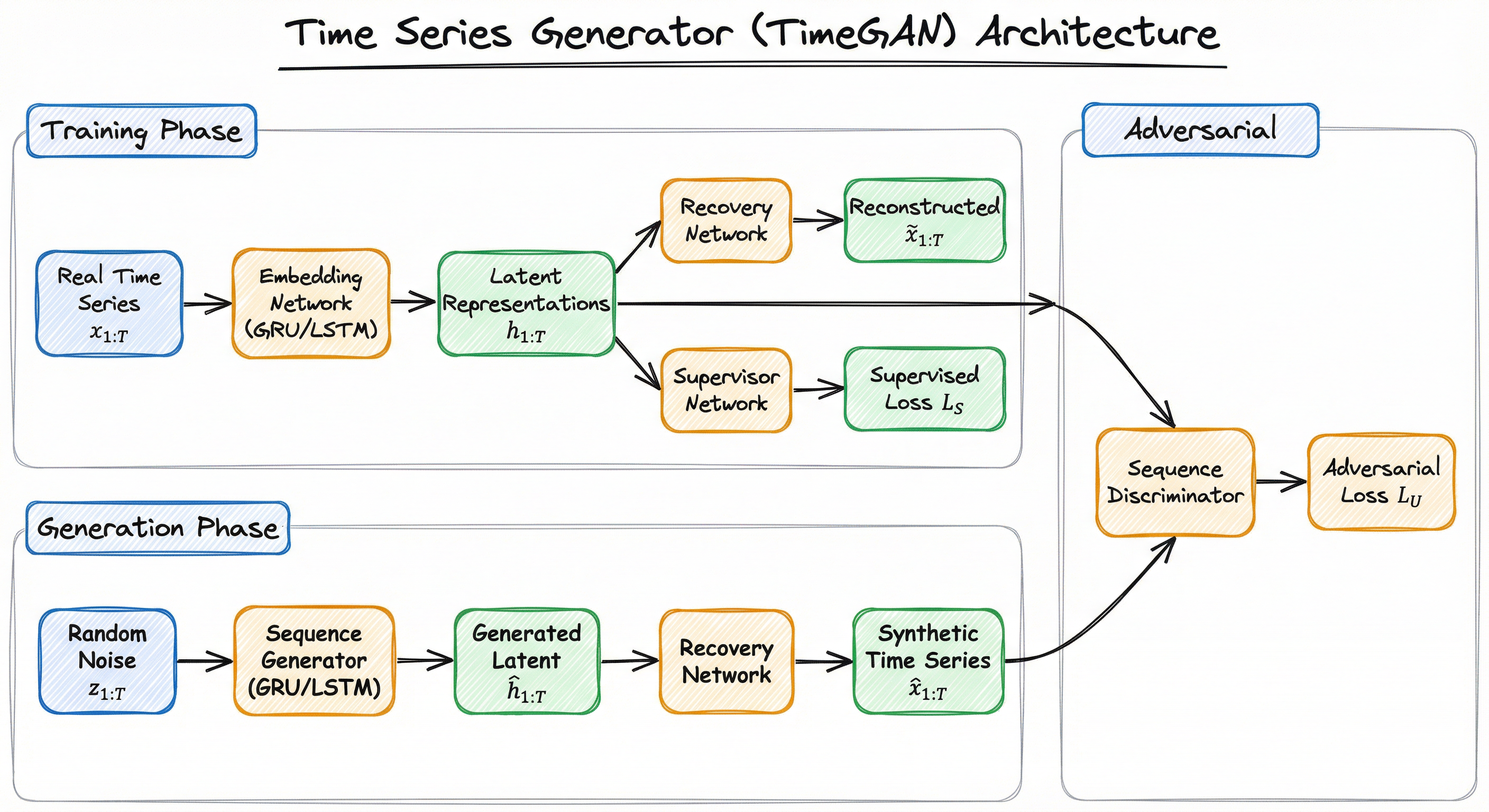
The embedding and recovery networks form an autoencoder that learns a smooth latent space. The generator operates in this latent space (not directly in data space), which simplifies the generation task. The supervisor network provides explicit temporal supervision in latent space, ensuring that generated trajectories follow plausible transition dynamics.
Key Components
Embedding Network
A recurrent neural network (typically GRU or LSTM) that maps the raw input time series into a latent representation . This creates a lower-dimensional space where temporal dynamics are easier to model. The embedding network is trained jointly with the recovery network as an autoencoder, ensuring the latent space preserves sufficient information for faithful reconstruction.
Recovery Network
The decoder counterpart to the embedding network. Takes latent representations (either from real data via the embedding network or from the generator) and maps them back to data space . Uses the same recurrent architecture as the embedding network but in reverse. The reconstruction loss ensures the autoencoder faithfully preserves the data.
Sequence Generator
A recurrent network that takes random noise vectors as input and produces synthetic latent trajectories . Critically, the generator operates autoregressively in latent space: at each step , it conditions on the previous generated latent state and the current noise . This autoregressive structure is what enables the generator to produce temporally coherent sequences.
Supervisor Network
A small auxiliary network that learns the one-step-ahead mapping in latent space: given , predict . This provides a supervised signal that explicitly encourages the generator to match the real temporal transitions. Without the supervisor, the generator only receives the coarse sequence-level adversarial signal, which is often insufficient for capturing fine-grained temporal dynamics.
Sequence Discriminator
A recurrent network that processes a latent sequence and classifies it as real (from the embedding network) or fake (from the generator). Unlike image discriminators that output a single scalar, the sequence discriminator can output per-step or per-subsequence scores, providing richer gradient signal to the generator.
Conditional Context Module (Optional)
In architectures like DoppelGANger and PAR, an additional module handles static context variables -- metadata that doesn't change across the sequence (e.g., sensor type, patient demographics, asset class). The context is generated first, then the temporal generator conditions on it. This separation of static and dynamic attributes improves generation quality for datasets with mixed-type metadata.
Data Flow
Training Flow: Real time series sequences are fed through the embedding network to produce latent representations. These latent representations serve three purposes: (1) they are passed to the recovery network for reconstruction (autoencoder path), (2) they provide supervision targets for the supervisor network (temporal dynamics path), and (3) they serve as positive examples for the discriminator (adversarial path). Simultaneously, the generator takes random noise and produces synthetic latent sequences, which the discriminator evaluates against the real latent sequences. All four networks are trained jointly with a combined objective.
Generation Flow: Random noise vectors are fed to the sequence generator, which autoregressively produces latent representations . These are then decoded through the recovery network to produce synthetic time series in the original data space. Optionally, the context module first generates static metadata, which conditions the temporal generation.
Evaluation Flow: Both real and synthetic sequences are evaluated using statistical tests (Kolmogorov-Smirnov, MMD), autocorrelation comparison, and downstream task performance (TSTR).
The architecture diagram shows the TimeGAN framework with four interconnected networks: an Embedding Network that encodes real time series into latent space, a Recovery Network that decodes back to data space, a Sequence Generator that produces synthetic latent trajectories from noise, and a Sequence Discriminator that distinguishes real from generated latent sequences. A Supervisor Network provides additional temporal supervision. The training phase uses real data through the autoencoder path, while the generation phase uses noise through the generator and recovery network.
How to Implement
Implementation Landscape
Time series generation implementation spans a spectrum from classical statistical methods to deep learning frameworks. The right choice depends on your data complexity, available compute, and quality requirements.
For simple, well-understood domains (e.g., generating seasonal demand patterns or ARIMA-like financial returns), statistical methods are often sufficient and dramatically faster to train. A well-fitted ARIMA model can generate thousands of sequences in seconds on a single CPU core.
For complex, multivariate, nonlinear dynamics (e.g., multi-sensor IoT streams, multi-asset financial portfolios, medical time series with irregular patterns), deep learning approaches like TimeGAN or DoppelGANger are necessary. These require GPU training (typically 1-4 hours on a single NVIDIA A100 for medium-sized datasets) but produce higher-fidelity synthetic data.
For production deployment at scale, frameworks like SDV (with the PAR synthesizer) and ydata-synthetic provide battle-tested APIs that handle data preprocessing, model training, and sampling in a unified pipeline. Gretel.ai's DGAN (based on DoppelGANger) offers a managed cloud service starting at ~$50/month (~INR 4,200/month) that eliminates infrastructure management.
Cost Note: Training a TimeGAN on a dataset of 10,000 sequences of length 24 with 5 features takes approximately 30-60 minutes on an NVIDIA T4 GPU (cloud cost: ~$0.50 or ~INR 42 per training run). For comparison, an ARIMA-based generator for the same task takes under 10 seconds on a CPU and costs effectively nothing.
import numpy as np
import pandas as pd
from ydata_synthetic.synthesizers.timeseries import TimeSeriesSynthesizer
from ydata_synthetic.preprocessing.timeseries import processed_stock

# Load and prepare real stock data
stock_data = processed_stock(seq_len=24)  # 24-step sequences
n_seq, seq_len, n_features = stock_data.shape
print(f"Training data: {n_seq} sequences, length {seq_len}, {n_features} features")

# Configure TimeGAN
gan_args = {
    "batch_size": 128,
    "lr": 5e-4,
    "noise_dim": 32,
    "layers_dim": 128,
    "latent_dim": 24,
    "gamma": 1.0,  # Weight of supervised loss
}

# Initialize and train
synth = TimeSeriesSynthesizer(
    modelname="timegan",
    model_parameters=gan_args,
)
synth.fit(
    stock_data,
    train_steps=5000,
    seq_len=seq_len,
    n_seq=n_features,
)

# Generate synthetic sequences
synthetic_data = synth.sample(n_samples=1000)
print(f"Generated: {synthetic_data.shape}")

# Validate: compare autocorrelation
from statsmodels.tsa.stattools import acf
real_acf = acf(stock_data[:, :, 0].flatten(), nlags=20)
syn_acf = acf(synthetic_data[:, :, 0].flatten(), nlags=20)
max_acf_diff = np.max(np.abs(real_acf - syn_acf))
print(f"Max ACF difference (first 20 lags): {max_acf_diff:.4f}")
This example uses the ydata-synthetic library to train a TimeGAN on stock price data. The key parameter is gamma which controls the weight of the supervised (temporal) loss relative to the adversarial loss. Higher gamma values enforce stronger temporal fidelity but may reduce diversity. The validation step compares autocorrelation functions -- a max ACF difference below 0.05 typically indicates good temporal fidelity.
import pandas as pd
from sdv.sequential import PARSynthesizer
from sdv.metadata import Metadata

# Prepare sequential data with entity context
data = pd.DataFrame({
    "sensor_id": ["S1"] * 100 + ["S2"] * 100,
    "timestamp": list(pd.date_range("2025-01-01", periods=100, freq="h")) * 2,
    "temperature": np.random.normal(25, 5, 200) + np.sin(np.linspace(0, 8*np.pi, 200)) * 3,
    "humidity": np.random.normal(60, 10, 200) + np.cos(np.linspace(0, 8*np.pi, 200)) * 5,
    "location": ["Mumbai"] * 100 + ["Bengaluru"] * 100,  # static context
})

# Define metadata
metadata = Metadata.detect_from_dataframe(data)
metadata.set_sequence_key("sensor_id")
metadata.set_sequence_index("timestamp")

# Train PAR model
synthesizer = PARSynthesizer(
    metadata,
    epochs=128,
    sample_size=1,
    cuda=True,
    verbose=True,
)
synthesizer.fit(data)

# Generate synthetic sequences for new entities
synthetic = synthesizer.sample(num_sequences=50)
print(f"Generated {synthetic['sensor_id'].nunique()} synthetic sensor streams")
print(synthetic.head(10))

# Save model for reuse
synthesizer.save("par_iot_model.pkl")
The PAR (Probabilistic Auto-Regressive) model from SDV handles sequential data with context. It separates static attributes (location, sensor type) from temporal attributes (temperature, humidity) and generates them independently. The sequence_key identifies different entities (sensors), and sequence_index defines the temporal ordering. PAR is significantly faster to train than TimeGAN and works well for medium-complexity time series with clear entity-level structure.
import numpy as np
import pandas as pd
from statsmodels.tsa.arima.model import ARIMA
from arch import arch_model

def fit_arima_garch(series: pd.Series, arima_order=(1,1,1), garch_order=(1,1)):
    """Fit ARIMA for mean dynamics + GARCH for volatility dynamics."""
    # Step 1: Fit ARIMA for the conditional mean
    arima_fit = ARIMA(series, order=arima_order).fit()
    residuals = arima_fit.resid

    # Step 2: Fit GARCH on residuals for volatility clustering
    garch = arch_model(residuals, vol="Garch", p=garch_order[0], q=garch_order[1])
    garch_fit = garch.fit(disp="off")

    return arima_fit, garch_fit

def generate_synthetic(arima_fit, garch_fit, n_steps=252, n_samples=100):
    """Generate synthetic time series with realistic volatility clustering."""
    synthetic_series = []

    for _ in range(n_samples):
        # Generate GARCH volatility path
        garch_sim = garch_fit.simulate(n_steps)
        innovations = garch_sim["data"].values

        # Generate ARIMA path with GARCH innovations
        arima_sim = arima_fit.simulate(n_steps, anchor="end",
                                        exog=None, repetitions=1)
        # Combine: ARIMA mean + GARCH-scaled residuals
        combined = arima_sim.values.flatten()
        synthetic_series.append(combined)

    return np.array(synthetic_series)

# Example: Generate synthetic Nifty50-like daily returns
nifty_returns = pd.Series(np.random.normal(0.0005, 0.015, 1000))  # placeholder
arima_fit, garch_fit = fit_arima_garch(nifty_returns)
synthetic = generate_synthetic(arima_fit, garch_fit, n_steps=252, n_samples=500)
print(f"Generated {synthetic.shape[0]} synthetic return series of {synthetic.shape[1]} days")
This classical approach combines ARIMA for mean dynamics with GARCH for volatility clustering -- the two most important features of financial time series. No GPU required, trains in seconds, and produces sequences with realistic fat tails and volatility persistence. For well-understood domains like financial returns, this often outperforms deep learning approaches on fidelity metrics while being orders of magnitude faster. The ARIMA+GARCH combination captures the stylized facts of financial data: mean reversion, volatility clustering, and leverage effects.
from gretel_synthetics.timeseries_dgan.dgan import DGAN
from gretel_synthetics.timeseries_dgan.config import DGANConfig
import numpy as np

# Prepare multivariate time series: (n_examples, n_timesteps, n_features)
# Example: IoT sensor data with 3 channels, 720 timesteps (30 days hourly)
n_examples = 500
n_timesteps = 720
n_features = 3

# Simulated IoT data with diurnal patterns and trends
t = np.linspace(0, 30*2*np.pi, n_timesteps)
real_data = np.zeros((n_examples, n_timesteps, n_features))
for i in range(n_examples):
    phase = np.random.uniform(0, 2*np.pi)
    amp = np.random.uniform(0.8, 1.2)
    real_data[i, :, 0] = amp * np.sin(t + phase) + np.random.normal(0, 0.1, n_timesteps)
    real_data[i, :, 1] = amp * np.cos(t + phase) * 0.5 + np.random.normal(0, 0.05, n_timesteps)
    real_data[i, :, 2] = np.cumsum(np.random.normal(0, 0.01, n_timesteps))  # random walk

# Configure DoppelGANger
config = DGANConfig(
    max_sequence_len=n_timesteps,
    sample_len=24,  # generate 24 steps at a time (batch size for LSTM)
    batch_size=min(100, n_examples),
    epochs=300,
    apply_feature_scaling=True,
    apply_example_scaling=False,
    use_attribute_discriminator=True,
)

# Train
model = DGAN(config=config)
model.train_numpy(real_data)

# Generate
synthetic_data = model.generate_numpy(100)
print(f"Synthetic data shape: {synthetic_data.shape}")

# Validate cross-correlation preservation
from scipy.stats import pearsonr
real_corr = pearsonr(real_data[:, :, 0].flatten(), real_data[:, :, 1].flatten())[0]
syn_corr = pearsonr(synthetic_data[:, :, 0].flatten(), synthetic_data[:, :, 1].flatten())[0]
print(f"Cross-correlation (real): {real_corr:.3f}, (synthetic): {syn_corr:.3f}")
DoppelGANger (DGAN) excels at long multivariate sequences where standard RNN-based generators struggle. The key parameter is sample_len -- the number of time steps generated per LSTM cell output. This batched generation approach captures long-range dependencies better than generating one step at a time. The use_attribute_discriminator enables separate discrimination of static attributes, improving quality for data with mixed static/temporal features. For IoT data with 720+ time steps, DGAN typically outperforms TimeGAN on autocorrelation preservation.
# TimeGAN training configuration (YAML)
model:
  type: timegan
  embedding_dim: 128
  hidden_dim: 128
  num_layers: 3
  noise_dim: 32
  gamma: 1.0  # supervised loss weight

training:
  epochs: 5000
  batch_size: 128
  learning_rate: 0.0005
  optimizer: adam
  sequence_length: 24

data:
  preprocessing:
    normalize: minmax  # or standard
    difference: true   # for non-stationary data
    fill_missing: forward_fill
  validation_split: 0.1

evaluation:
  metrics:
    - discriminative_score
    - predictive_score
    - autocorrelation_diff
    - mmd
  acf_max_lags: 50
  tstr_model: lstm_classifier
Common Implementation Mistakes
- ●
Ignoring stationarity requirements: Many time series generators assume (weakly) stationary input data. Feeding raw non-stationary series (e.g., stock prices with trends) without differencing or detrending leads to generators that overfit to the training period's trend rather than learning reusable dynamics. Always difference or normalize your data first, then reverse the transformation on synthetic output.
- ●
Using sequence-level metrics only: Evaluating synthetic time series by comparing marginal distributions (histograms, KS tests) without checking temporal properties (autocorrelation, cross-correlation, spectral density) gives a false sense of quality. Shuffled real data would pass marginal tests but be temporally useless.
- ●
Setting sequence length too long for recurrent generators: TimeGAN and RGAN struggle with sequences longer than ~100-200 steps due to gradient vanishing in LSTMs/GRUs. For longer sequences, use DoppelGANger's batched generation or split into overlapping windows and stitch.
- ●
Training with too few sequences: Deep generative models need sufficient diversity in training examples. Training TimeGAN on 50 sequences of length 100 will produce memorized copies. Aim for at least 500-1,000 training sequences, or use data windowing to create overlapping subsequences from longer recordings.
- ●
Neglecting feature scaling: Multivariate time series often have features at very different scales (e.g., temperature in 20-45 range and humidity in 40-90 range). Without per-feature normalization, the generator's loss is dominated by the large-scale feature, producing poor results on small-scale features. Always normalize to [0,1] or [-1,1] per feature before training.
When Should You Use This?
Use When
You need to augment a small time series dataset for training forecasting or anomaly detection models -- especially when rare events (crashes, failures, anomalies) are underrepresented
Privacy regulations prevent sharing raw temporal data (healthcare vitals, financial transactions, energy consumption patterns) but you need synthetic data for collaborative research or model development
You are building simulation environments for reinforcement learning agents that interact with temporal processes (trading bots, supply chain optimizers, industrial control systems)
Stress testing requires generating synthetic scenarios that go beyond historical observations -- e.g., simulating NSE market conditions more extreme than any observed crash for risk model validation
You need to create balanced training datasets where certain temporal patterns (device failures, patient deterioration events, fraud sequences) are rare in real data
Data collection is ongoing but models need to be trained now -- synthetic data can bootstrap initial model training before sufficient real data accumulates
Avoid When
Your real dataset is already large and representative (>100K sequences with good coverage of relevant scenarios). The marginal benefit of synthetic data diminishes rapidly with dataset size.
The downstream task is sensitive to exact distributional properties that are hard to validate -- e.g., if you're computing Value at Risk and even small distributional errors translate to regulatory violations, synthetic data introduces unquantified risk
The time series has complex regime-switching behavior that the generator cannot capture -- running a generator that misses regime changes is worse than using the limited real data, because it creates false confidence in model robustness
You need synthetic data that is exactly privacy-safe (differential privacy guarantees). Most time series generators do not provide formal privacy guarantees -- you need dedicated DP-SGD training or PATE frameworks for that
The temporal dynamics are driven by exogenous variables not present in your training data -- a generator trained only on stock prices without macro indicators will produce sequences that violate fundamental economic relationships
Your evaluation pipeline lacks time series-specific metrics (ACF comparison, spectral analysis, TSTR). Without proper evaluation, you cannot assess whether the synthetic data is useful or harmful.
Key Tradeoffs
Fidelity vs. Privacy
The fundamental tradeoff in time series generation is between fidelity (how closely the synthetic data matches the real distribution) and privacy (how well individual real sequences are protected from reconstruction). Higher fidelity means the generator has learned more about the training data, which inherently increases privacy risk. Adding noise or using differential privacy during training improves privacy guarantees but degrades fidelity.
For Indian healthcare applications under the DPDP Act 2023, you need to decide where on this spectrum your use case falls. For medical research collaboration (e.g., AIIMS sharing synthetic ECG data with IIT researchers), moderate fidelity with strong privacy is appropriate. For internal data augmentation where the same team has access to the real data anyway, maximum fidelity is the priority.
Complexity vs. Training Cost
| Approach | Training Time | GPU Required | Quality (Complex Data) | Quality (Simple Data) |
|---|---|---|---|---|
| ARIMA/GARCH | Seconds | No | Medium | High |
| PAR (SDV) | 5-30 min | Optional | Medium-High | High |
| TimeGAN | 30-120 min | Yes | High | High |
| DoppelGANger | 1-4 hours | Yes | High (long sequences) | Medium-High |
| GT-GAN | 2-6 hours | Yes | Very High (irregular) | High |
For a Bengaluru startup running on a budget of INR 50,000/month for compute, PAR or ARIMA might be the pragmatic choice. For a well-funded fintech like Zerodha or a research lab at IISc, TimeGAN or DoppelGANger on GPU instances is justifiable.
Sequence Length vs. Quality
Recurrent generators degrade as sequence length increases. For sequences under 100 steps, most methods work well. For 100-500 steps, DoppelGANger's batched generation or windowed approaches are needed. For 500+ steps, consider hierarchical generation (generate coarse patterns first, then fill in details) or non-recurrent architectures like temporal convolutional networks.
Alternatives & Comparisons
A standard GAN generates data points independently without temporal structure. Use a standard GAN when your data is tabular or image-based with no sequential dependencies. Use a time series generator when your data has temporal ordering and autocorrelation that must be preserved. If you flatten a time series into a vector and feed it to a standard GAN, you lose all temporal structure.
CTGAN specializes in tabular data with mixed continuous and categorical columns. It treats each row independently. For time series, CTGAN can generate individual time steps with correct marginal distributions but cannot capture temporal dependencies. Use CTGAN for cross-sectional tabular data; use a time series generator for sequential data where the order matters.
Standard VAEs generate data points independently like GANs. However, temporal VAEs (TimeVAE) add autoregressive structure to the decoder, making them a viable alternative to TimeGAN. TimeVAE is typically faster to train and more stable than adversarial approaches, but may produce slightly less sharp outputs. Choose TimeVAE when training stability is critical; choose TimeGAN when maximum fidelity is required.
Diffusion models for time series (TimeGrad, CSDI) are emerging as strong alternatives to GAN-based generators. They avoid mode collapse entirely and provide better coverage of the data distribution. However, they are significantly slower at generation time (requiring hundreds of denoising steps vs. a single forward pass for GANs). Choose diffusion when quality matters more than generation speed.
Gaussian generators sample from parametric multivariate normal distributions. They can model linear correlations but cannot capture nonlinear dynamics, heavy tails, or regime switches in time series. Use Gaussian generators as a quick baseline or when your time series is approximately Gaussian (e.g., stable sensor readings). For anything with complex temporal dynamics, use a dedicated time series generator.
Pros, Cons & Tradeoffs
Advantages
Preserves temporal dependencies -- unlike tabular generators, time series generators explicitly model autocorrelation, seasonality, and cross-variable temporal relationships, producing sequences that are usable for downstream forecasting and anomaly detection tasks
Enables privacy-preserving data sharing -- synthetic time series allows organizations to share data patterns without exposing individual records, critical for Indian healthcare (DPDP Act) and financial (RBI guidelines) compliance
Augments rare event scenarios -- generates plausible crash scenarios, equipment failures, or disease progression patterns that are underrepresented in real data, improving model robustness for tail-risk estimation
Reduces data collection costs -- training on a mix of real and synthetic data can achieve comparable downstream performance with 3-5x less real data, saving significant costs in sensor deployment, clinical trials, or market data subscriptions (NSE data feeds cost ~INR 2-5 lakh/year for real-time access)
Supports simulation and stress testing -- enables Monte Carlo-style scenario analysis by generating thousands of plausible trajectories, useful for VaR calculations, capacity planning, and what-if analysis without waiting for rare real events
Multiple maturity levels available -- from simple ARIMA/GARCH models that require no GPU to advanced TimeGAN/DoppelGANger frameworks, teams can choose the right complexity level for their data and budget
Disadvantages
Temporal fidelity is hard to validate -- marginal distribution tests can pass while temporal dynamics are completely wrong; requires specialized metrics (ACF comparison, spectral density matching, TSTR) that many teams lack expertise to implement properly
Training instability with adversarial approaches -- TimeGAN and DoppelGANger inherit GAN training challenges (mode collapse, oscillation) compounded by the sequential nature of the data; hyperparameter tuning is more difficult than for tabular GANs
Sequence length limitations -- recurrent generators degrade beyond ~200 steps; DoppelGANger's batched approach extends this but introduces artifacts at batch boundaries; very long series (1000+ steps) remain challenging
No formal privacy guarantees by default -- standard time series generators can memorize and reproduce training sequences, especially with small training sets; differential privacy integration exists but significantly degrades generation quality
Multivariate scaling challenges -- generation quality degrades as the number of features increases beyond ~10-15; high-dimensional multivariate time series (50+ channels of IoT sensors) require dimensionality reduction before generation, adding pipeline complexity
Domain expertise still required -- the generator needs appropriate preprocessing (differencing, normalization, windowing) that requires domain knowledge; a poorly preprocessed input produces misleading synthetic data regardless of the model's sophistication
Failure Modes & Debugging
Temporal mode collapse
Cause
The generator converges to producing a single repeating pattern or a small set of stereotypical trajectories, ignoring the diversity of temporal dynamics in the training data. This is more common than mode collapse in image GANs because time series distributions are often multimodal (e.g., weekday vs. weekend patterns, bull vs. bear market regimes).
Symptoms
All generated sequences look nearly identical. The diversity metric (e.g., average pairwise DTW distance between synthetic sequences) is significantly lower than between real sequences. The synthetic data covers only one mode of the training distribution -- for example, only generating calm market periods and never volatile ones.
Mitigation
Use Wasserstein loss (WGAN-GP) instead of standard GAN loss. Increase the noise dimension to provide more random variation. Implement mini-batch discrimination. Monitor diversity metrics during training and apply early stopping when diversity plateaus. For financial data, ensure training data includes examples from multiple market regimes.
Autocorrelation structure mismatch
Cause
The generator captures marginal distributions correctly but fails to reproduce the temporal dependency structure. This happens when the supervised loss weight () is too low, the latent dimension is insufficient, or the recurrent network lacks capacity to model the autocorrelation structure.
Symptoms
Histogram comparisons between real and synthetic data look good, but the ACF/PACF of synthetic data diverges from real data, especially at lags 1-10. Downstream forecasting models trained on synthetic data perform significantly worse than those trained on real data (TSTR gap > 15%).
Mitigation
Increase the supervised loss weight . Compare ACF plots at multiple lags during training as a validation metric. Use longer hidden state dimensions in the recurrent components. For data with strong seasonality, ensure the sequence length is at least 2x the seasonal period to allow the model to observe complete cycles.
Distribution leakage (privacy failure)
Cause
The generator memorizes specific training sequences rather than learning the underlying distribution. This is especially likely with small training sets (<200 sequences) or when training for too many epochs without regularization.
Symptoms
Some generated sequences are near-exact copies of training sequences (DTW distance to nearest neighbor in training set approaches zero). A membership inference attack achieves high accuracy (>70%) in distinguishing sequences that were in the training set from those that weren't.
Mitigation
Monitor nearest-neighbor distance between synthetic and real sequences during training. Implement early stopping based on this metric. Use dropout and weight decay as regularization. For sensitive data, add differential privacy to the training loop (DP-SGD) or use PATE-GAN. Limit training epochs -- for medical data at AIIMS or financial data at banks, err on the side of under-training rather than over-training.
Non-stationarity amplification
Cause
The generator is trained on non-stationary data (e.g., raw stock prices with upward trends) and amplifies the trend in synthetic data, producing sequences with unrealistic drift. The model overfits to the specific trend direction observed in the training window rather than learning stationary dynamics.
Symptoms
Synthetic sequences exhibit exaggerated trends -- prices growing exponentially, sensor readings drifting far beyond physical bounds. The variance of endpoint values across synthetic sequences is much larger than in real data.
Mitigation
Always apply differencing or detrending before training. Generate synthetic returns/differences, then reconstruct levels by applying the synthetic differences to a realistic starting point. Verify that the training data passes an ADF stationarity test before feeding it to the generator. For financial data, work with log-returns rather than raw prices.
Cross-variable correlation destruction
Cause
In multivariate time series, the generator learns each variable's marginal temporal dynamics but fails to preserve the correlation structure between variables. This is common when features are normalized independently or when the generator architecture processes variables in parallel without cross-attention.
Symptoms
Each variable individually looks realistic, but variable pairs exhibit incorrect correlation patterns. For IoT data, physically linked sensors (temperature and energy consumption) show no correlation in synthetic data. For financial data, correlated assets (HDFC Bank and ICICI Bank stocks) move independently in synthetic sequences.
Mitigation
Use joint multivariate generation (not per-variable generation). Validate cross-correlation matrices between real and synthetic data. For DoppelGANger, ensure apply_example_scaling=False so that cross-variable relationships are preserved rather than normalized away. Add a cross-correlation loss term if using a custom architecture.
Batch boundary artifacts (DoppelGANger-specific)
Cause
DoppelGANger's batched generation approach divides long sequences into chunks of sample_len steps, each produced by a single LSTM output. At chunk boundaries, there can be discontinuities or unnatural transitions because the model transitions between independently generated batches.
Symptoms
Periodic artifacts in synthetic sequences at intervals matching the sample_len parameter. Visible discontinuities or sudden regime changes every 24 steps (if sample_len=24). The spectral density shows anomalous peaks at frequencies corresponding to the batch length.
Mitigation
Set sample_len to divide evenly into the total sequence length. Choose sample_len that aligns with natural periodicities in the data (e.g., 24 for hourly data with daily cycles). Post-process with light smoothing at batch boundaries if artifacts persist. Consider overlapping generation with blending at boundaries.
Placement in an ML System
Where It Sits in the ML Pipeline
The time series generator typically sits between data collection/storage and model training. In a typical workflow:
- Real time series data is collected from sensors, APIs, or databases (upstream: time-series-db, feature-store)
- The generator is trained on this real data (possibly after validation and preprocessing)
- Synthetic time series is generated and merged with real data for downstream consumption
- The combined dataset feeds into feature engineering and model training
Integration Patterns
Pattern 1: Offline Augmentation -- Generate synthetic data once, store it alongside real data, and use the combined dataset for all downstream training. This is the simplest pattern and works when data distribution is relatively stable.
Pattern 2: Online Augmentation -- Generate synthetic sequences on-the-fly during training, similar to image augmentation. This provides unlimited training data diversity but requires the generator to be fast enough for inline use (PAR and small TimeGANs work; large DoppelGANgers don't).
Pattern 3: Scenario Generation -- Use the generator to create specific scenarios (stress tests, what-if analyses) for evaluation rather than training. The generated data feeds into evaluation pipelines rather than training pipelines.
Key Insight: The time series generator is both a data multiplier (augmenting small datasets) and a privacy shield (enabling data sharing without exposing originals). Its placement in the pipeline reflects whichever role is primary for your use case.
Pipeline Stage
Data Generation / Augmentation
Upstream
- time-series-db
- data-validator
- feature-store
Downstream
- feature-engineer
- data-validator
- model-trainer
Scaling Bottlenecks
The primary bottleneck is training time, which scales linearly with dataset size and quadratically with sequence length for recurrent models. A TimeGAN training run on 10K sequences of length 100 takes ~45 minutes on an A100 GPU. Scaling to 100K sequences pushes this to ~4-6 hours. For DoppelGANger on sequences of length 1000+, expect 8-12 hours of training on a single GPU.
Once trained, generation is fast but still sequential for recurrent models: each time step depends on the previous one, preventing parallelization within a single sequence. Generating 10K sequences of length 100 takes ~30 seconds for TimeGAN, ~2 minutes for DoppelGANger. For batch generation of millions of sequences (e.g., Monte Carlo simulation), consider parallelizing across multiple GPU workers.
Recurrent generators hold hidden states for all time steps during backpropagation through time (BPTT). For sequences of length 1000 with hidden dimension 256, this requires ~1 GB of GPU memory per batch element. Batch size is therefore limited by GPU memory, not compute, for long sequences.
On an NVIDIA A100 (80 GB): max batch size ~256 for sequences of length 100, ~64 for length 500, ~16 for length 2000. Training throughput: ~500 sequences/second for TimeGAN, ~200 sequences/second for DoppelGANger.
Production Case Studies
JPMorgan's AI Research team developed synthetic financial time series generators for risk model validation and stress testing. They used GAN-based approaches to generate synthetic market scenarios that preserve the statistical properties of real financial data -- including fat tails, volatility clustering, and cross-asset correlations. The synthetic data is used to stress-test trading algorithms and risk models beyond the limited set of historical market crises.
Reduced reliance on historical scenarios for stress testing by generating 10,000+ synthetic market crash scenarios. Risk model coverage improved by 40% for tail events that had no historical precedent. The approach enabled validation of models against scenarios more extreme than any observed in 50+ years of market data.
Philips Research used TimeGAN and recurrent GAN architectures to generate synthetic patient vital signs (heart rate, blood pressure, respiratory rate, SpO2) for ICU monitoring algorithm development. The synthetic data enabled external research collaborations without exposing protected health information (PHI), while preserving the clinically relevant temporal patterns needed for early warning score development.
Generated synthetic ICU datasets of 50,000+ patient stays used by 12 external research groups. Models trained on synthetic data achieved within 3% AUC of models trained on real data for sepsis prediction. Eliminated a 6-month data sharing agreement process that had previously bottlenecked research collaborations.
Siemens used synthetic time series generation for predictive maintenance of gas turbines. Real sensor data from turbine operations was used to train DoppelGANger-style generators that could produce synthetic failure sequences -- critical because actual turbine failures are extremely rare (perhaps 2-3 per year across a fleet of 100 turbines). The synthetic failure data augmented training sets for anomaly detection models.
Augmented the training dataset with 5,000 synthetic failure sequences per failure mode. Anomaly detection recall improved from 67% to 89% on held-out real failure events. Reduced false alarm rate by 35%, saving an estimated $2.1 million (~INR 17.6 crore) annually in unnecessary inspection costs across the turbine fleet.
American Express researchers explored GAN-based synthetic time series generation for credit card transaction sequence modeling. They used temporal GANs to generate synthetic transaction sequences that preserve spending patterns, temporal correlations between transactions, and the statistical signatures of fraudulent activity. This enabled training fraud detection models on balanced datasets where real fraud sequences are extremely rare (<0.1% of transactions).
Fraud detection models trained on augmented datasets (real + synthetic) showed a 12% improvement in fraud detection rate at the same false positive rate compared to models trained on real data alone with traditional oversampling. The synthetic data approach was particularly effective for detecting novel fraud patterns not well-represented in historical data.
Tooling & Ecosystem
Python library implementing TimeGAN, DoppelGANger, and other generative models for both tabular and time series data. Built on TensorFlow 2.0. Provides a unified API for training and generating synthetic time series with built-in evaluation metrics. The most popular open-source option for TimeGAN-based generation.
The PAR (Probabilistic Auto-Regressive) synthesizer from SDV handles sequential data with context variables. Supports multi-entity time series (multiple sensors, patients, accounts) with both static and temporal attributes. Significantly faster to train than adversarial approaches. Part of the broader SDV ecosystem by DataCebo.
Gretel's open-source implementation of DoppelGANger optimized for time series data. Provides a clean API with configurable sequence length, sample length, and feature scaling. Now part of NVIDIA (acquired 2025). Available as both open-source library and managed cloud service. Handles long multivariate sequences better than most alternatives.
Comprehensive Python framework for time series generation and evaluation. Implements GANs, VAEs, and probabilistic models. Includes 140+ built-in datasets, augmentation utilities, and evaluation metrics (discriminative score, predictive score, privacy metrics). Published at NeurIPS 2024. The most research-oriented option with strong evaluation tooling.
Classical statistical time series modeling. statsmodels provides ARIMA, SARIMAX, and state-space models. The arch package adds GARCH, EGARCH, and other volatility models. Together, they enable statistical time series generation that requires no GPU, trains in seconds, and works well for data with known parametric structure. Often the right first baseline.
SDV's dedicated library for mixed-type, multivariate time series generation. Supports both PAR and neural network-based sequence models. Handles categorical temporal variables (event types, states) alongside continuous measurements. Good for log-like data with mixed types.
Research & References
Yoon, Jarrett & van der Schaar (2019)NeurIPS 2019
Introduced TimeGAN, combining adversarial training with a stepwise supervised loss and autoencoder framework. The supervised loss explicitly captures temporal transition dynamics, addressing a key weakness of applying standard GANs to sequential data. Demonstrated on medical, financial, and synthetic benchmark time series.
Lin, Jain, Wang, Fanti & Sekar (2020)ACM IMC 2020 (Best Paper Finalist)
Introduced DoppelGANger, which uses batched LSTM generation where each cell outputs multiple time steps, significantly improving long-range dependency capture. Addresses challenges of mixed static and temporal attributes with a separate attribute discriminator. Achieved 43% better fidelity than baseline GAN approaches.
Esteban, Hyland & Rätsch (2017)arXiv preprint (ICLR 2017 Workshop)
Pioneering work applying recurrent neural networks in GAN generator and discriminator for medical time series. Introduced RGAN and RCGAN architectures with the Train on Synthetic, Test on Real (TSTR) evaluation framework. Demonstrated on ICU patient data from PhysioNet.
Jeon, Kim, Park, Choi & Lee (2022)NeurIPS 2022
First general-purpose model for both regular and irregular time series synthesis. Uses neural ODEs and continuous-time flow processes to handle missing data and irregular sampling intervals. Outperforms TimeGAN and DoppelGANger on both regular and irregular benchmarks.
Wiese, Knobloch, Korn & Kretschmer (2020)Quantitative Finance, Vol. 20, No. 9
Applied temporal convolutional networks (TCNs) to generate financial time series that capture long-range dependencies including volatility clustering, leverage effects, and serial autocorrelation. The generator architecture allows explicit transition to risk-neutral distributions for derivative pricing.
Desai, Freeman, Wang & Beaver (2021)arXiv preprint
Proposed a VAE architecture with interpretable components for time series generation. Incorporates domain-specific patterns (polynomial trends, seasonalities) directly into the decoder architecture. Achieves comparable quality to TimeGAN with significantly faster and more stable training.
Nikitin, Iannucci & Kaski (2024)NeurIPS 2024 (Datasets and Benchmarks)
Presented a unified Python framework for time series generation and evaluation. Implements multiple generative models (GANs, VAEs, probabilistic) with standardized evaluation metrics. Includes 140+ built-in datasets for benchmarking and comprehensive privacy analysis tools.
Interview & Evaluation Perspective
Common Interview Questions
- ●
How would you generate synthetic time series data for training a forecasting model when you only have 6 months of historical data?
- ●
What's the difference between using a standard GAN and TimeGAN for time series generation? Why does the supervised loss matter?
- ●
How do you evaluate whether synthetic time series data is good enough for downstream model training?
- ●
Describe how you'd generate synthetic market data for stress testing a trading algorithm at a fintech like Zerodha.
- ●
What are the privacy implications of using GAN-generated synthetic time series in healthcare? How would you ensure compliance with data protection regulations?
- ●
When would you use classical statistical methods (ARIMA/GARCH) vs. deep learning approaches (TimeGAN/DoppelGANger) for time series generation?
Key Points to Mention
- ●
TimeGAN's key innovation is the supervised loss that explicitly captures stepwise temporal transitions, not just sequence-level adversarial realism. This is what separates it from naively applying a GAN to flattened sequences.
- ●
Always evaluate synthetic time series using temporal metrics (autocorrelation function comparison, spectral density matching, TSTR predictive performance) -- marginal distribution comparisons alone are insufficient and misleading.
- ●
For financial time series, highlight the stylized facts that must be preserved: fat tails, volatility clustering (GARCH effects), leverage effects, and mean reversion. A generator that misses these produces useless synthetic data for risk applications.
- ●
DoppelGANger's batched generation (producing
sample_lensteps per LSTM output) is architecturally motivated: it helps capture long-range dependencies that standard step-by-step RNN generation struggles with. - ●
Start with the simplest approach that works: ARIMA+GARCH for financial returns, seasonal decomposition for demand data. Deep learning generators are justified when the data has complex nonlinear dynamics that statistical models cannot capture.
Pitfalls to Avoid
- ●
Claiming that synthetic time series has formal privacy guarantees without implementing differential privacy -- standard TimeGAN/DoppelGANger can memorize training sequences and have no provable privacy properties.
- ●
Evaluating synthetic time series quality only with marginal distribution tests (KS test, histograms) and ignoring temporal fidelity metrics. This is the most common mistake and leads to false confidence in generator quality.
- ●
Treating time series generation as a solved problem -- it's not. Long sequences (1000+ steps), high-dimensional multivariate data (50+ channels), and regime-switching dynamics remain actively challenging.
- ●
Forgetting to mention preprocessing requirements: differencing for non-stationarity, normalization per feature, and minimum training set size. These are practical details that separate working implementations from failed projects.
Senior-Level Expectation
A senior/staff-level candidate should discuss the full lifecycle: data preprocessing (stationarity testing, normalization), model selection (matching architecture to data complexity and sequence length), training strategy (loss balancing, early stopping criteria), comprehensive evaluation (temporal fidelity, diversity, privacy, TSTR), and production integration (offline vs. online augmentation, versioning synthetic datasets, drift monitoring between real and synthetic distributions over time). They should be able to reason about cost-quality tradeoffs specific to the domain -- for example, explaining why ARIMA+GARCH is often superior to TimeGAN for generating financial return series, or why DoppelGANger is better suited than TimeGAN for IoT data with 500+ step sequences. Bonus points for discussing connections to diffusion-based time series generation as the likely future direction, and for articulating formal privacy guarantees (or the lack thereof) in current approaches.
Summary
A time series generator is a generative model that learns temporal dynamics from real sequential data and produces synthetic sequences preserving the statistical properties, autocorrelations, and conditional distributions of the original data. It addresses three critical challenges in ML systems: data scarcity (especially for rare events like market crashes or equipment failures), privacy constraints (enabling data sharing without exposing individual records), and simulation needs (generating thousands of plausible scenarios for stress testing and Monte Carlo analysis).
The field spans classical statistical approaches (ARIMA, GARCH) that are fast and interpretable but limited to simple dynamics, through modern deep learning methods (TimeGAN, DoppelGANger, PAR) that capture complex nonlinear temporal patterns. TimeGAN's key innovation is the supervised temporal loss that explicitly captures stepwise transition dynamics. DoppelGANger excels at long sequences through batched generation. PAR from SDV offers a lightweight, production-ready option with context variable support. The choice depends on data complexity, sequence length, and computational budget.
Evaluation of synthetic time series requires going beyond marginal distribution tests to include temporal fidelity metrics (autocorrelation comparison, spectral density matching) and downstream utility (Train on Synthetic, Test on Real). Common failure modes include temporal mode collapse, autocorrelation mismatch, and privacy leakage through memorization. For production deployment, teams must decide between offline augmentation (generate once, store alongside real data) and online augmentation (generate on-the-fly during training), balancing generation quality against latency and compute cost.
Time series generation is fundamentally harder than tabular synthesis because temporal dependencies are the signal, not noise. A generator that ignores them produces data that is worse than useless -- it provides false confidence in model robustness. Start simple (ARIMA for well-understood dynamics), validate thoroughly (ACF comparison is non-negotiable), and scale complexity only when the data demands it.