GAN Data Generator in Machine Learning
Generative Adversarial Networks (GANs) represent one of the most revolutionary breakthroughs in machine learning since their introduction by Ian Goodfellow and colleagues in 2014. At their core, GANs pit two neural networks against each other in a competitive game: a generator that learns to create synthetic data, and a discriminator that learns to distinguish real data from fake. This adversarial dynamic drives both networks to improve -- the generator creates increasingly realistic samples while the discriminator becomes more discerning.
The elegance of GANs lies in their game-theoretic foundation. Unlike traditional generative models that require explicit probability density estimation (often intractable for high-dimensional data), GANs learn to generate data through competition. The generator doesn't need to model directly; it only needs to fool the discriminator. This indirect approach has enabled GANs to generate photorealistic images, synthesize human speech, create molecular structures for drug discovery, and produce privacy-preserving synthetic datasets for sensitive domains like healthcare and finance.
Since 2014, the GAN landscape has exploded with innovations addressing the original framework's notorious training instability. DCGAN (Deep Convolutional GAN) introduced architectural best practices for image generation. WGAN (Wasserstein GAN) replaced the problematic JS-divergence with a more stable distance metric. StyleGAN enabled unprecedented control over generated image attributes. CTGAN brought GAN-based synthesis to tabular data, enabling synthetic datasets that preserve complex statistical relationships in structured data.
Today, GANs power everything from Flipkart's product image generation to AIIMS Delhi's privacy-preserving medical data synthesis. They're the backbone of creative AI tools used by Indian design studios, enable data augmentation for startups with limited labeled data, and provide the foundation for privacy-preserving data sharing in regulated industries.
Concept Snapshot
- What It Is
- A framework where two neural networks -- a generator and a discriminator -- compete in a minimax game, with the generator learning to produce synthetic data that is indistinguishable from real data while the discriminator learns to classify samples as real or fake.
- Category
- Data Generation
- Complexity
- Advanced
- Inputs / Outputs
- Inputs: training dataset + random noise vector (latent code). Outputs: synthetic samples that match the statistical distribution of the training data.
- System Placement
- Sits in the data generation and augmentation stage of ML pipelines, typically before feature engineering or as a standalone synthetic data generator for privacy-preserving data sharing.
- Also Known As
- Generative Adversarial Network, GAN, Adversarial Generator, GAN-based Data Synthesizer
- Typical Users
- ML Engineers, Data Scientists, Computer Vision Engineers, Privacy Engineers, Research Scientists, MLOps Engineers
- Prerequisites
- Deep neural networks (feedforward, convolutional), Backpropagation and gradient descent optimization, Game theory basics (minimax, Nash equilibrium), Probability distributions and sampling, PyTorch or TensorFlow fundamentals
- Key Terms
- generatordiscriminatorminimax objectivemode collapsetraining instabilityNash equilibriumWasserstein distanceconditional GANlatent space
Why This Concept Exists
The Challenge of Generative Modeling
Before GANs, generative modeling was dominated by approaches that required explicit density estimation: modeling the probability of the data directly. Methods like Gaussian Mixture Models worked for simple, low-dimensional data but failed catastrophically for high-dimensional distributions like natural images. Variational Autoencoders (VAEs) made progress but produced blurry samples because they optimized pixel-wise reconstruction loss rather than perceptual quality.
The fundamental challenge was intractable normalization. Most interesting probability distributions have partition functions that are computationally infeasible to compute in high dimensions. Energy-based models could define unnormalized distributions, but training them required expensive MCMC sampling or contrastive divergence -- techniques that struggled to scale to complex data.
The Breakthrough: Competition Instead of Density
In 2014, Ian Goodfellow had a key insight during a debate with colleagues at a Montreal bar. What if, instead of explicitly modeling , we trained a generator network to fool a learned discriminator? The discriminator would act as an adaptive loss function, automatically learning what makes data realistic rather than relying on hand-crafted metrics like L2 distance.
This adversarial framing bypassed the intractable density problem entirely. The generator maps noise to data space , while the discriminator outputs the probability that came from real data rather than the generator. The two networks play a minimax game: the generator tries to maximize the discriminator's error rate, while the discriminator tries to minimize it.
The original GAN paper (Goodfellow et al., 2014) showed that this adversarial training converges to a Nash equilibrium where the generator's distribution matches the real data distribution , and the discriminator can do no better than random guessing ( everywhere).
From Theory to Practice: The Rocky Road
The initial excitement around GANs was tempered by severe practical challenges. Training was notoriously unstable -- models would collapse to generating a single repeated sample (mode collapse), oscillate without converging, or produce nonsensical outputs. The minimax objective required careful balancing of the generator and discriminator learning rates.
The research community responded with a wave of innovations:
- DCGAN (2015): Radford et al. introduced architectural guidelines (use strided convolutions, batch normalization, LeakyReLU) that dramatically stabilized training for image generation.
- WGAN (2017): Arjovsky et al. replaced the JS-divergence with Wasserstein distance, providing a meaningful training loss that correlates with sample quality.
- Progressive GAN (2017): Karras et al. grew networks progressively from low to high resolution, enabling 1024×1024 face generation.
- StyleGAN (2018-2020): Introduced style-based generator architecture and adaptive instance normalization, achieving unprecedented image quality and controllability.
Indian Context: Research groups at IIT Delhi, IISc Bangalore, and IIT Bombay have contributed to GAN research, particularly in applications like medical image synthesis (AIIMS collaboration), agricultural data augmentation for crop disease detection, and privacy-preserving financial data synthesis for Indian fintech compliance.
Core Intuition & Mental Model
The Counterfeiter and the Detective
The classic analogy for GANs is a counterfeiter (generator) trying to produce fake currency that can fool a detective (discriminator). At first, the counterfeiter produces crude fakes -- obvious forgeries. The detective easily spots them and explains why: wrong paper texture, incorrect watermarks, poor color matching.
The counterfeiter uses this feedback to improve. Second-generation fakes have better textures and colors. But the detective, having seen these improved fakes, becomes more discerning -- noticing subtler flaws like incorrect serial number patterns or slightly off ink composition.
This back-and-forth escalates. The counterfeiter's fakes become better and better. The detective becomes more and more expert at spotting fakes. Eventually, if training succeeds, the counterfeiter produces bills that are indistinguishable from real currency, and the detective can do no better than flipping a coin.
The Two-Network Dance
Here's what's happening mechanically:
-
Generator's turn: Take random noise (the "creative spark" -- pure randomness with no structure). Pass it through the generator network to produce a synthetic sample .
-
Discriminator's evaluation: Feed both real samples from the dataset and generated samples to the discriminator. The discriminator outputs -- the probability that is real.
-
Discriminator training: Update the discriminator to increase (correctly identify real data) and decrease (correctly identify fakes). This makes the discriminator a better "fraud detector."
-
Generator training: Here's the clever part -- update the generator to maximize . That is, make the discriminator think the fakes are real. The generator's gradients flow through the discriminator -- the discriminator acts as a learned, adaptive loss function.
-
Repeat: This adversarial training continues for thousands of iterations. If successful, the generator learns the true data distribution.
Why Noise?
The random noise serves as the "source of creativity." If the generator had no random input, it could only produce a single deterministic output -- not useful. The noise provides diversity: different random seeds produce different outputs, all of which should look realistic. The generator learns to map the latent space (the space of noise vectors ) to the data space in a way that covers the real data distribution.
Mental Model: Think of the latent space as a "space of concepts" and the generator as a renderer. For face generation, one dimension of might control "age," another "gender," another "expression." The generator learns this semantic structure implicitly through adversarial training.
Technical Foundations
The Minimax Objective
A GAN consists of two functions:
- Generator: mapping latent codes to data space
- Discriminator: outputting the probability that input is real
The training objective is a minimax game:
The discriminator maximizes by correctly classifying real data () and fake data (). The generator minimizes by producing samples that the discriminator classifies as real ().
Global Optimum
At the optimal solution, the generator perfectly replicates the data distribution: . When this occurs, the discriminator cannot distinguish real from fake and outputs for all . The global minimum of the objective is:
Connection to JS-Divergence
The original GAN objective minimizes the Jensen-Shannon divergence between and :
where is the mixture distribution. The problem: JS-divergence saturates when the supports of and don't overlap -- leading to vanishing gradients in the generator.
Non-Saturating Loss (Practical Variant)
In practice, the generator uses a non-saturating objective to avoid vanishing gradients in early training when :
This is equivalent to minimizing:
which provides stronger gradients when the discriminator is confident that samples are fake.
Wasserstein GAN (WGAN)
To address training instability, WGAN uses the Wasserstein-1 distance (Earth Mover's distance):
Under the Kantorovich-Rubinstein duality, this can be expressed as:
where is a 1-Lipschitz function. In WGAN, the discriminator (now called a critic) is constrained to be 1-Lipschitz through weight clipping or gradient penalty.
WGAN with Gradient Penalty (WGAN-GP)
Improved Training of Wasserstein GANs (Gulrajani et al., 2017) replaces weight clipping with a gradient penalty term:
where with samples along straight lines between real and generated data. The penalty (typically 10) enforces the 1-Lipschitz constraint more effectively than weight clipping.
Convergence Guarantee: Unlike the original GAN objective, the Wasserstein distance is continuous everywhere and differentiable almost everywhere, providing more stable gradients throughout training.
Internal Architecture
The GAN architecture consists of two adversarial neural networks trained simultaneously. The generator transforms random noise into synthetic samples through a series of learned transformations. The discriminator processes both real and generated samples to output a probability score indicating authenticity.
For image generation, the generator typically uses transposed convolutions (or upsampling + convolution) to progressively increase spatial resolution from a low-dimensional latent code. The discriminator mirrors this with strided convolutions that progressively downsample to a single classification score.
The following diagram shows the bidirectional information flow during training:
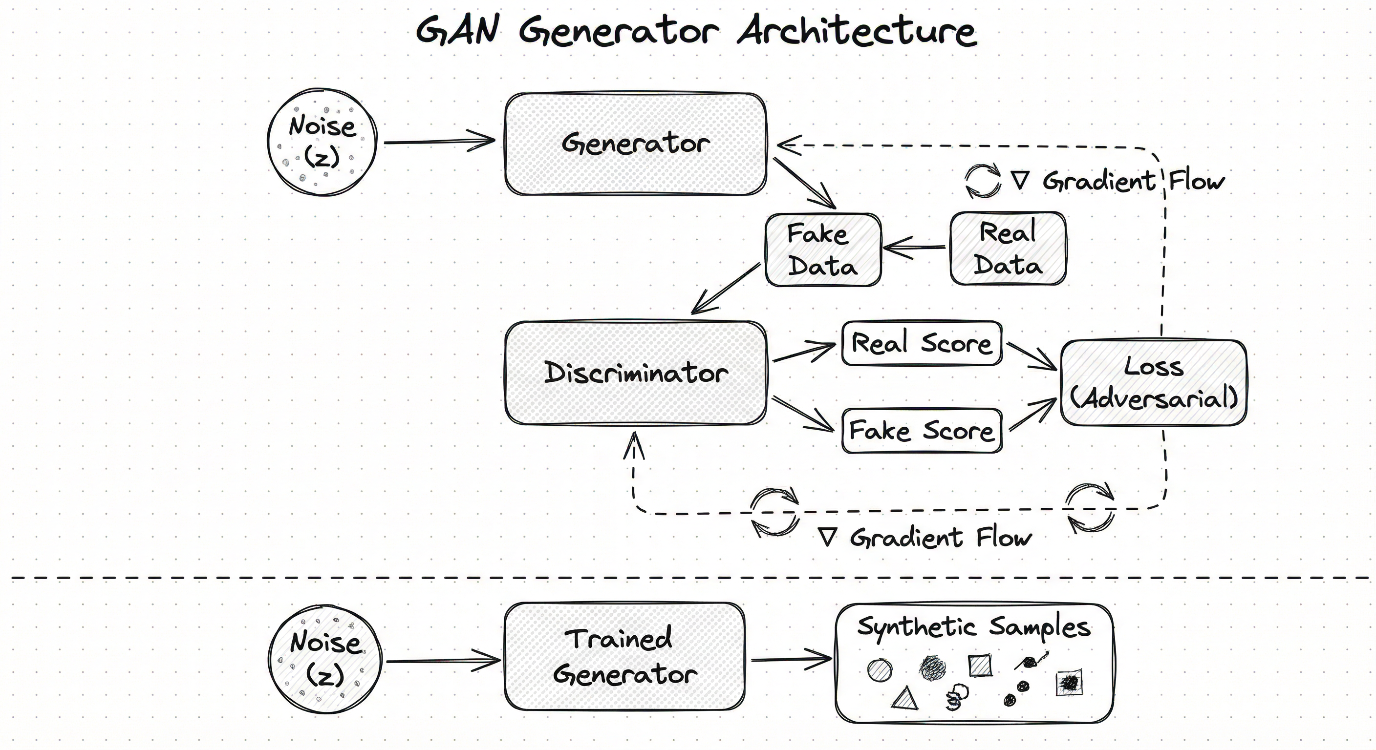
The discriminator is updated more frequently (typically 5x) than the generator to maintain its effectiveness as a learned loss function. This prevents the generator from exploiting a weak discriminator.
Key Components
Generator Network
A neural network that maps latent codes to synthetic data . For images, typically uses transposed convolutions with batch normalization and ReLU activations (except the output layer which uses tanh). The architecture progressively upsamples from a small spatial size (e.g., 4×4) to the target resolution (e.g., 64×64, 256×256). Modern variants like StyleGAN use adaptive instance normalization (AdaIN) to inject style information at each resolution.
Discriminator Network
A neural network that classifies inputs as real or fake. For images, uses strided convolutions (no pooling) with LeakyReLU activations and optionally batch normalization or layer normalization. Outputs a single scalar through a sigmoid activation (original GAN) or no activation (WGAN). Acts as an adaptive, learned loss function that provides gradients to the generator.
Latent Space
The input space from which the generator samples noise vectors . Typically with dimension 64-512. The generator learns to map this unstructured space to a structured manifold in data space. In conditional GANs, the latent code is concatenated with class labels or other conditioning information.
Loss Functions
The adversarial objectives that drive training. Standard GAN uses binary cross-entropy. Non-saturating GAN maximizes for the generator. WGAN uses Wasserstein distance with Lipschitz constraint. WGAN-GP adds gradient penalty. LSGAN (Least Squares GAN) uses L2 loss for more stable gradients. The choice of loss significantly impacts training stability and sample quality.
Batch Normalization / Layer Normalization
Normalization layers that stabilize training by preventing covariate shift. Batch normalization is standard in DCGAN discriminators but can cause artifacts in small-batch settings. Layer normalization or spectral normalization are alternatives. Critically, batch norm statistics should NOT be shared between real and fake samples in the discriminator -- this can leak information and destabilize training.
Conditional Inputs (cGAN)
Optional class labels, text embeddings, or other conditioning information concatenated with in the generator and with in the discriminator. Enables controlled generation: "generate a sample of class " or "generate a face with attributes ." Class embeddings are typically learned jointly during training. Used in CTGAN for tabular data to condition on column values.
Data Flow
Training Iteration Flow:
-
Sample real data: Draw a minibatch of real samples from the training dataset.
-
Generate fake data: Sample noise vectors from the latent distribution (typically standard normal). Pass through generator: .
-
Discriminator forward pass: Compute for real samples and for generated samples.
-
Discriminator training: Compute discriminator loss (e.g., ) and backpropagate to update discriminator parameters . This is typically done k times (k=5 for WGAN) per generator update.
-
Generator training: Sample new noise and generate . Compute discriminator scores . Compute generator loss (e.g., ). Backpropagate through the discriminator (with discriminator weights frozen) to update generator parameters .
-
Repeat: Continue alternating discriminator and generator updates for many epochs.
Key Detail: The generator never sees real data directly. It only receives gradients through the discriminator, which acts as a proxy for "how to improve realism."
Inference Flow: At inference time, only the generator is used. Sample , compute , output . No discriminator is needed for generation.
A flowchart showing the GAN training loop. Random noise enters the generator (green) to produce fake samples. Both real data and fake samples feed into the discriminator (orange). The discriminator outputs probability scores, which feed into two loss functions: discriminator loss (red) that updates the discriminator to better distinguish real from fake, and generator loss (blue) that backpropagates through the frozen discriminator to update the generator. Dotted lines show the parameter update paths creating a feedback loop.
How to Implement
Implementation Approaches
There are three main paths to implementing GANs in production:
Approach 1: PyTorch/TensorFlow from Scratch -- For research or custom architectures, implement the generator and discriminator as nn.Module subclasses and manually orchestrate the training loop. This provides maximum control but requires careful engineering to handle the alternating updates and gradient flow.
Approach 2: High-Level Libraries -- For tabular data, use SDV (Synthetic Data Vault) with CTGAN or TVAE. For images, use frameworks like PyTorch-GAN or TensorFlow GAN that provide pre-built architectures (DCGAN, WGAN-GP, StyleGAN2). These abstract away low-level details while remaining customizable.
Approach 3: Commercial Platforms -- Tools like Gretel.ai, MOSTLY AI, or Tonic.ai provide GUI-based GAN training for synthetic data generation, particularly for tabular/relational data with privacy guarantees. Best for non-technical teams or compliance-focused use cases.
Training Stability Techniques
GAN training requires careful engineering to avoid failure modes:
- Architecture design: Follow DCGAN guidelines (stride convolutions, batch norm, LeakyReLU).
- Discriminator updates: Train discriminator 5x per generator update (WGAN standard).
- Gradient penalty: Use WGAN-GP instead of weight clipping for Lipschitz constraint.
- Label smoothing: Use soft labels (0.9 instead of 1.0 for real data) to prevent discriminator overconfidence.
- Spectral normalization: Normalize weight matrices by their largest singular value to enforce Lipschitz constraint.
- Two time-scale update rule (TTUR): Use different learning rates for generator and discriminator (e.g., , ).
Cost Note: Training a DCGAN on 64×64 images with a dataset of 50K samples takes ~2 hours on a single RTX 4090 (~INR 170 / 800-1,200 (~INR 67,000-1,00,000) for a full training run on 8x V100s over 3-5 days.
import torch
import torch.nn as nn
import torch.optim as optim
from torch.utils.data import DataLoader
from torchvision import datasets, transforms

# Hyperparameters
latent_dim = 100
image_size = 64
channels = 3
batch_size = 128
lr = 0.0002
beta1 = 0.5  # Adam parameter for GANs

# Generator
class Generator(nn.Module):
    def __init__(self):
        super().__init__()
        self.main = nn.Sequential(
            # Input: latent_dim x 1 x 1 -> 512 x 4 x 4
            nn.ConvTranspose2d(latent_dim, 512, 4, 1, 0, bias=False),
            nn.BatchNorm2d(512),
            nn.ReLU(True),
            # 512 x 4 x 4 -> 256 x 8 x 8
            nn.ConvTranspose2d(512, 256, 4, 2, 1, bias=False),
            nn.BatchNorm2d(256),
            nn.ReLU(True),
            # 256 x 8 x 8 -> 128 x 16 x 16
            nn.ConvTranspose2d(256, 128, 4, 2, 1, bias=False),
            nn.BatchNorm2d(128),
            nn.ReLU(True),
            # 128 x 16 x 16 -> 64 x 32 x 32
            nn.ConvTranspose2d(128, 64, 4, 2, 1, bias=False),
            nn.BatchNorm2d(64),
            nn.ReLU(True),
            # 64 x 32 x 32 -> 3 x 64 x 64
            nn.ConvTranspose2d(64, channels, 4, 2, 1, bias=False),
            nn.Tanh()  # Output in [-1, 1]
        )

    def forward(self, z):
        return self.main(z)

# Discriminator
class Discriminator(nn.Module):
    def __init__(self):
        super().__init__()
        self.main = nn.Sequential(
            # 3 x 64 x 64 -> 64 x 32 x 32
            nn.Conv2d(channels, 64, 4, 2, 1, bias=False),
            nn.LeakyReLU(0.2, inplace=True),
            # 64 x 32 x 32 -> 128 x 16 x 16
            nn.Conv2d(64, 128, 4, 2, 1, bias=False),
            nn.BatchNorm2d(128),
            nn.LeakyReLU(0.2, inplace=True),
            # 128 x 16 x 16 -> 256 x 8 x 8
            nn.Conv2d(128, 256, 4, 2, 1, bias=False),
            nn.BatchNorm2d(256),
            nn.LeakyReLU(0.2, inplace=True),
            # 256 x 8 x 8 -> 512 x 4 x 4
            nn.Conv2d(256, 512, 4, 2, 1, bias=False),
            nn.BatchNorm2d(512),
            nn.LeakyReLU(0.2, inplace=True),
            # 512 x 4 x 4 -> 1 x 1 x 1
            nn.Conv2d(512, 1, 4, 1, 0, bias=False),
            nn.Sigmoid()
        )

    def forward(self, x):
        return self.main(x).view(-1, 1)

# Initialize models
device = torch.device('cuda' if torch.cuda.is_available() else 'cpu')
generator = Generator().to(device)
discriminator = Discriminator().to(device)

# Optimizers
optim_G = optim.Adam(generator.parameters(), lr=lr, betas=(beta1, 0.999))
optim_D = optim.Adam(discriminator.parameters(), lr=lr, betas=(beta1, 0.999))

# Loss
criterion = nn.BCELoss()

# Training loop
for epoch in range(num_epochs):
    for i, (real_imgs, _) in enumerate(dataloader):
        batch_size = real_imgs.size(0)
        real_imgs = real_imgs.to(device)

        # Labels
        real_labels = torch.ones(batch_size, 1).to(device)
        fake_labels = torch.zeros(batch_size, 1).to(device)

        # ---------------------
        #  Train Discriminator
        # ---------------------
        optim_D.zero_grad()

        # Real images
        real_output = discriminator(real_imgs)
        d_loss_real = criterion(real_output, real_labels)

        # Fake images
        z = torch.randn(batch_size, latent_dim, 1, 1).to(device)
        fake_imgs = generator(z)
        fake_output = discriminator(fake_imgs.detach())
        d_loss_fake = criterion(fake_output, fake_labels)

        # Total discriminator loss
        d_loss = d_loss_real + d_loss_fake
        d_loss.backward()
        optim_D.step()

        # -----------------
        #  Train Generator
        # -----------------
        optim_G.zero_grad()

        # Generate fake images (reuse z or sample new)
        z = torch.randn(batch_size, latent_dim, 1, 1).to(device)
        fake_imgs = generator(z)
        fake_output = discriminator(fake_imgs)

        # Generator wants discriminator to think fakes are real
        g_loss = criterion(fake_output, real_labels)
        g_loss.backward()
        optim_G.step()
This is the canonical DCGAN implementation. Key architectural choices:
- Transposed convolutions in generator with stride=2 for upsampling (no pooling)
- Batch normalization after each layer except generator output and discriminator input
- ReLU in generator (except output which uses tanh to match [-1,1] image range)
- LeakyReLU (slope=0.2) in discriminator to prevent dead neurons
- Adam optimizer with learning rate 0.0002 and beta1=0.5 (lower momentum for stability)
- Separate forward passes for real and fake in discriminator to avoid batch norm issues
- Detach fake images when training discriminator to prevent gradients flowing to generator
import torch
import torch.nn as nn
import torch.optim as optim
import torch.autograd as autograd

# WGAN-GP uses critic (no sigmoid) instead of discriminator
class Critic(nn.Module):
    def __init__(self):
        super().__init__()
        self.model = nn.Sequential(
            nn.Conv2d(3, 64, 4, 2, 1),
            nn.LayerNorm([64, 32, 32]),  # LayerNorm instead of BatchNorm
            nn.LeakyReLU(0.2),
            nn.Conv2d(64, 128, 4, 2, 1),
            nn.LayerNorm([128, 16, 16]),
            nn.LeakyReLU(0.2),
            nn.Conv2d(128, 256, 4, 2, 1),
            nn.LayerNorm([256, 8, 8]),
            nn.LeakyReLU(0.2),
            nn.Conv2d(256, 1, 8, 1, 0),  # No sigmoid!
        )

    def forward(self, x):
        return self.model(x).view(-1)

def compute_gradient_penalty(critic, real_samples, fake_samples, device):
    """Compute gradient penalty for WGAN-GP."""
    batch_size = real_samples.size(0)

    # Random weight for interpolation
    alpha = torch.rand(batch_size, 1, 1, 1).to(device)

    # Interpolate between real and fake samples
    interpolates = (alpha * real_samples + (1 - alpha) * fake_samples).requires_grad_(True)

    # Critic scores for interpolated samples
    d_interpolates = critic(interpolates)

    # Compute gradients
    gradients = autograd.grad(
        outputs=d_interpolates,
        inputs=interpolates,
        grad_outputs=torch.ones_like(d_interpolates),
        create_graph=True,
        retain_graph=True,
    )[0]

    # Flatten gradients
    gradients = gradients.view(batch_size, -1)

    # Compute gradient penalty
    gradient_penalty = ((gradients.norm(2, dim=1) - 1) ** 2).mean()
    return gradient_penalty

# Hyperparameters
lambda_gp = 10  # Gradient penalty coefficient
n_critic = 5     # Train critic 5 times per generator update

# Training loop modifications
for epoch in range(num_epochs):
    for i, (real_imgs, _) in enumerate(dataloader):
        real_imgs = real_imgs.to(device)

        # ---------------------
        #  Train Critic
        # ---------------------
        for _ in range(n_critic):
            optim_C.zero_grad()

            # Generate fake images
            z = torch.randn(batch_size, latent_dim, 1, 1).to(device)
            fake_imgs = generator(z)

            # Critic outputs (no sigmoid, can be any real number)
            real_validity = critic(real_imgs)
            fake_validity = critic(fake_imgs.detach())

            # Wasserstein loss
            critic_loss = -torch.mean(real_validity) + torch.mean(fake_validity)

            # Gradient penalty
            gp = compute_gradient_penalty(critic, real_imgs, fake_imgs, device)

            # Total critic loss
            c_loss = critic_loss + lambda_gp * gp
            c_loss.backward()
            optim_C.step()

        # -----------------
        #  Train Generator
        # -----------------
        optim_G.zero_grad()

        z = torch.randn(batch_size, latent_dim, 1, 1).to(device)
        fake_imgs = generator(z)
        fake_validity = critic(fake_imgs)

        # Generator wants to maximize critic output for fake images
        g_loss = -torch.mean(fake_validity)
        g_loss.backward()
        optim_G.step()
WGAN-GP improves on standard GAN and WGAN with key changes:
- No sigmoid in critic -- outputs unrestricted real numbers representing Wasserstein distance
- LayerNorm instead of BatchNorm to avoid batch-dependent statistics
- Gradient penalty enforces 1-Lipschitz constraint more effectively than weight clipping
- Critic trained 5x per generator update to maintain optimal critic throughout
- Wasserstein loss: maximize difference between real and fake scores
- Interpolated samples: gradient penalty computed on linear interpolations between real and fake
This provides much more stable training and meaningful loss curves (lower is better, correlates with sample quality).
from sdv.single_table import CTGANSynthesizer
from sdv.metadata import SingleTableMetadata
import pandas as pd

# Load real tabular data
real_data = pd.read_csv('customer_data.csv')

# Define metadata (column types, constraints)
metadata = SingleTableMetadata()
metadata.detect_from_dataframe(real_data)

# Optionally specify column types explicitly
metadata.update_column(
    column_name='age',
    sdtype='numerical',
    computer_representation='Int64'
)
metadata.update_column(
    column_name='income',
    sdtype='numerical',
    computer_representation='Float'
)
metadata.update_column(
    column_name='country',
    sdtype='categorical'
)
metadata.set_primary_key('customer_id')

# Initialize CTGAN synthesizer
synthesizer = CTGANSynthesizer(
    metadata,
    epochs=300,
    batch_size=500,
    generator_dim=(256, 256),
    discriminator_dim=(256, 256),
    generator_lr=2e-4,
    discriminator_lr=2e-4,
    discriminator_steps=1,
    verbose=True
)

# Train the GAN
print("Training CTGAN on real data...")
synthesizer.fit(real_data)

# Generate synthetic data
num_synthetic_rows = 10000
synthetic_data = synthesizer.sample(num_rows=num_synthetic_rows)

print(f"Generated {len(synthetic_data)} synthetic rows")
print(synthetic_data.head())

# Save model and synthetic data
synthesizer.save('models/ctgan_customer.pkl')
synthetic_data.to_csv('synthetic_customer_data.csv', index=False)

# Evaluate quality
from sdv.evaluation.single_table import evaluate_quality

quality_report = evaluate_quality(
    real_data,
    synthetic_data,
    metadata
)

print(f"Quality Score: {quality_report.get_score():.2f}")
quality_report.get_details(property_name='Column Shapes')
CTGAN (Conditional Tabular GAN) handles the unique challenges of tabular data:
- Mode-specific normalization: Mixed data types (continuous, categorical, ordinal) are normalized appropriately
- Conditional vector: Ensures all categories are generated (solves imbalanced class problem)
- Training-by-sampling: Samples each training batch based on categorical column distributions
- Metadata specification: Explicitly define column types, constraints, primary keys
SDV's CTGAN is production-ready with quality metrics (Column Shapes, Column Pair Trends) and privacy guarantees. Typical use cases: synthetic test data for development, privacy-preserving data sharing for compliance (GDPR, HIPAA), and data augmentation for rare classes.
# WGAN-GP Configuration (YAML)
model:
  architecture: wgan-gp
  latent_dim: 128
  image_size: 64
  channels: 3

generator:
  base_channels: 64
  num_layers: 4
  activation: relu
  output_activation: tanh
  normalization: batch_norm

critic:
  base_channels: 64
  num_layers: 4
  activation: leaky_relu
  normalization: layer_norm
  spectral_norm: false

training:
  batch_size: 64
  epochs: 200
  critic_iterations: 5
  gradient_penalty_lambda: 10
  learning_rate_generator: 1e-4
  learning_rate_critic: 4e-4
  optimizer: adam
  beta1: 0.0
  beta2: 0.9

data:
  dataset: celeba
  augmentation:
    - random_horizontal_flip
    - random_crop
    - normalize:
        mean: [0.5, 0.5, 0.5]
        std: [0.5, 0.5, 0.5]

checkpointing:
  save_every: 10
  num_samples: 64
  log_images: true
Common Implementation Mistakes
- ●
Training discriminator to completion early: If the discriminator becomes too strong too quickly (near-perfect accuracy), it provides zero gradients to the generator. The generator cannot learn. Solution: train discriminator and generator in a balanced way -- discriminator should be slightly better but not perfect. Use discriminator accuracy as a diagnostic: aim for 60-80%, not 95%+.
- ●
Using batch normalization incorrectly: Batch norm statistics should NOT be computed jointly over real and fake samples in the discriminator. This leaks information about the batch composition. Always separate forward passes:
D(real_batch)thenD(fake_batch). For small batches, consider layer normalization or spectral normalization instead. - ●
Ignoring mode collapse: When the generator produces limited diversity (e.g., 5 variations of faces instead of thousands), training has collapsed. Causes: discriminator overfitting, insufficient generator capacity, or poor architecture. Solutions: reduce discriminator capacity, increase generator capacity, use minibatch discrimination, or switch to WGAN-GP.
- ●
Wrong label smoothing: Using 1.0 for real and 0.0 for fake makes the discriminator overconfident. Use one-sided label smoothing: 0.9 for real (or sample from [0.8, 1.0]) and keep 0.0 for fake. Never smooth fake labels to 0.1 -- this teaches the discriminator that fakes are partially real.
- ●
Not monitoring loss curves correctly: In standard GAN, loss values oscillate and are NOT monotonically decreasing. This is expected -- it's a game, not optimization. The discriminator loss should oscillate around 0.69 (log(2), random guessing). If it goes to zero, the discriminator is too strong. If generator loss explodes, training has diverged. Use WGAN for interpretable loss curves.
- ●
Forgetting to detach fake samples when training discriminator:
fake_imgs = generator(z)creates a computational graph. When computing discriminator loss on fakes, usediscriminator(fake_imgs.detach())to prevent gradients flowing back to the generator. Only when training the generator should gradients flow through the discriminator.
When Should You Use This?
Use When
You need to generate high-dimensional synthetic data (images, audio, time series) where traditional generative models produce blurry or unrealistic outputs
You're doing data augmentation for a computer vision or NLP task and need diverse, realistic training samples beyond standard transformations
You need privacy-preserving synthetic data for sensitive domains (healthcare, finance) and cannot share real data due to GDPR, HIPAA, or other regulations
You have imbalanced datasets and need to synthesize minority class samples to improve classifier performance (GAN-based oversampling)
You're building creative AI tools for design, gaming, or media (image synthesis, texture generation, style transfer) where photorealism is critical
You need to learn implicit data distributions without manually specifying probability models (GANs discover the distribution through adversarial training)
You have sufficient compute resources (single GPU minimum for DCGAN, multi-GPU for StyleGAN) and can tolerate training instability
Avoid When
Your data is low-dimensional or simple -- for tabular data with <20 columns and simple relationships, consider VAEs or statistical methods (copulas) which are more stable
You have very limited training data (<1000 samples) -- GANs are data-hungry and will mode collapse on tiny datasets. Use data augmentation or few-shot learning instead
You need guaranteed convergence or reproducible training -- GAN training is stochastic and outcomes vary across runs. For mission-critical applications requiring determinism, use VAEs or diffusion models
You require density estimation or anomaly detection -- GANs don't model explicitly. Use VAEs, normalizing flows, or autoregressive models if you need likelihood values
Your team lacks deep learning expertise -- GAN debugging requires understanding gradients, game theory, and architectural nuances. For non-expert teams, use pre-trained models or commercial platforms
You need fast iteration cycles -- GAN training takes hours to days. For rapid prototyping, use rule-based synthesis, template-based generation, or pre-trained diffusion models (e.g., Stable Diffusion)
You're generating discrete sequences (text, code) -- GANs struggle with non-differentiable discrete outputs. Use autoregressive models (GPT), VAEs, or diffusion models instead
Key Tradeoffs
Core Tradeoff: Sample Quality vs. Training Stability
GANs are notorious for producing the highest-quality samples among generative models but at the cost of training difficulty. VAEs train stably but produce blurry images. Diffusion models match GAN quality with better stability but require 1000x more sampling steps at inference.
| Aspect | GAN | VAE | Diffusion Model |
|---|---|---|---|
| Sample Quality | Excellent (photorealistic) | Good (sometimes blurry) | Excellent (matches GANs) |
| Training Stability | Poor (mode collapse, divergence) | Excellent | Good |
| Training Time | Moderate (hours-days) | Fast (minutes-hours) | Slow (days-weeks) |
| Inference Speed | Fast (single forward pass) | Fast (single forward pass) | Slow (1000 denoising steps) |
| Density Estimation | No (implicit model) | Yes (explicit ) | Yes (via diffusion SDE) |
| Controllability | Moderate (latent interpolation) | Good (latent space structure) | Excellent (conditioning) |
Privacy vs. Utility Tradeoff
For privacy-preserving synthetic data, adding differential privacy (DP) to GAN training degrades sample quality. DP-CTGAN with (strong privacy) produces tabular data with ~10-20% lower downstream model accuracy compared to non-private CTGAN. Increasing to 10.0 (weak privacy) recovers most utility but provides weaker guarantees.
Compute Cost
GAN training cost scales with data complexity:
| Task | Resolution | Training Time | GPU Cost (Cloud) | Cost (INR) |
|---|---|---|---|---|
| MNIST digits | 28×28 | 1 hour | $1 (1x T4) | ₹85 |
| CIFAR-10 | 32×32 | 4 hours | $4 (1x V100) | ₹340 |
| CelebA faces | 64×64 | 12 hours | $12 (1x V100) | ₹1,000 |
| High-res faces | 256×256 | 2 days | $240 (4x V100) | ₹20,100 |
| StyleGAN2 1024×1024 | 1024×1024 | 5 days | $960 (8x V100) | ₹80,500 |
Practitioner's Note: For most production use cases, WGAN-GP on 64×64 or 128×128 images strikes the best balance. Higher resolutions rarely justify the 10-100x cost increase unless photorealism is critical (e.g., fashion e-commerce, design tools).
Alternatives & Comparisons
Variational Autoencoders (VAEs) train stably with a well-defined loss function and provide explicit density estimation . However, VAE samples tend to be blurrier than GAN samples due to the Gaussian prior and pixel-wise reconstruction loss. Choose VAEs when you need stable training, density estimation for anomaly detection, or are working with small datasets (<10K samples). Choose GANs when sample quality is paramount and you can afford the training complexity.
Diffusion models (DDPM, DDIM) achieve GAN-level sample quality with more stable training by learning a gradual denoising process. They support excellent conditioning and controllability. However, inference is 100-1000x slower than GANs due to iterative denoising (20-1000 steps). Choose diffusion models when training stability and sample quality are both critical and inference latency is acceptable. Choose GANs when real-time generation is required (e.g., interactive applications, video frame synthesis).
CTGAN is a specialized GAN variant for tabular data that handles mixed data types (continuous, categorical, ordinal) and imbalanced classes through mode-specific normalization and conditional vectors. It's the state-of-the-art for synthetic tabular data in the SDV library. Choose CTGAN over generic GANs when working with structured/tabular data. Choose generic GANs (DCGAN, StyleGAN) for image, audio, or unstructured data.
TVAE (Tabular VAE) is an alternative to CTGAN for tabular synthetic data, using a VAE architecture instead of GAN. TVAE trains more stably and quickly than CTGAN but may produce slightly lower quality samples for complex multivariate distributions. Choose TVAE when training stability and speed are more important than marginal quality gains. Choose CTGAN when achieving the highest statistical fidelity to the real data is critical (e.g., for regulatory compliance).
Autoregressive models (PixelCNN, WaveNet, GPT for text) decompose as a product of conditionals and generate sequentially. They provide exact likelihood computation and stable training but generate slowly (sequential sampling). Choose autoregressive models for discrete data (text, music notes), density estimation tasks, or when you need interpretable likelihoods. Choose GANs for fast parallel generation of continuous data.
Pros, Cons & Tradeoffs
Advantages
Exceptional sample quality: GANs produce the most photorealistic images, realistic audio, and high-fidelity synthetic data among generative models. StyleGAN2 faces are indistinguishable from real photos to human observers.
Fast inference: Generation requires only a single forward pass through the generator. A 64×64 DCGAN generates 1000 images in ~2 seconds on a GPU, enabling real-time applications.
No need for explicit density modeling: GANs learn implicit distributions through adversarial training, avoiding intractable partition functions and density estimation in high dimensions.
Flexible architecture: The adversarial framework is architecture-agnostic. You can use CNNs for images, RNNs for sequences, Transformers for any modality -- the discriminator acts as a universal learned loss function.
Privacy-preserving data generation: With differential privacy (DP-GAN, PATE-GAN), GANs generate synthetic datasets that provably protect individual privacy, enabling data sharing for medical research, financial analysis, and other sensitive domains under GDPR/HIPAA.
Excellent for creative applications: GANs power style transfer, super-resolution, image-to-image translation (pix2pix, CycleGAN), face editing, and game asset generation -- domains where perceptual quality trumps pixel-perfect accuracy.
Conditional generation: Conditional GANs (cGAN) enable controlled synthesis -- "generate a smiling face" or "synthesize a customer record with income > $100K" -- useful for data augmentation and targeted synthetic data creation.
Disadvantages
Notoriously unstable training: Mode collapse, vanishing gradients, and oscillating losses plague standard GAN training. Debugging requires expertise in neural network optimization, game theory, and architecture design. Training runs can fail after hours without clear diagnostics.
Mode collapse: The generator may collapse to producing a limited subset of the data distribution (e.g., 10 face variations instead of diverse faces). This limits diversity in synthetic data and makes GANs unsuitable for coverage-sensitive applications.
No density estimation: GANs don't provide , making them unsuitable for anomaly detection, outlier scoring, or tasks requiring likelihood values. You can't answer "how likely is this sample?" with a GAN.
Evaluation is subjective: Unlike VAEs (use ELBO) or autoregressive models (use perplexity), there's no universally accepted GAN evaluation metric. Inception Score and FID (Fréchet Inception Distance) are proxies but don't capture all aspects of generation quality. Visual inspection is still the gold standard.
Data-hungry: GANs require thousands to millions of training samples to learn complex distributions. For small datasets (<1000 samples), GANs overfit and produce memorized copies rather than novel samples. Transfer learning helps but doesn't eliminate the data requirement.
Difficult for discrete data: GANs rely on backpropagation through the generator, which requires differentiable operations. Generating discrete sequences (text tokens, DNA bases) requires workarounds like Gumbel-Softmax or reinforcement learning (SeqGAN), both of which are unstable.
Compute-intensive training: High-resolution GANs (StyleGAN at 1024×1024) require multi-GPU setups and days of training, costing $500-1,200 (~INR 42,000-1,00,000) per training run. This puts cutting-edge GANs out of reach for most Indian startups and research labs without cloud credits.
Failure Modes & Debugging
Mode Collapse
Cause
The generator discovers a limited set of samples that consistently fool the discriminator and ignores the rest of the data distribution. This occurs when the discriminator fails to provide diverse feedback or when the generator exploits a narrow weakness in the discriminator. Mathematically, the generator converges to a delta function on a single (or few) mode(s) of instead of covering the full distribution.
Symptoms
Generated samples lack diversity -- e.g., a face GAN produces 5-10 distinct faces repeated with minor variations instead of thousands of unique faces. Training loss may look normal (discriminator accuracy ~50-60%), but visual inspection reveals repetition. Quantitatively, low diversity scores (inverse of Inception Score) or high precision but low recall on FID.
Mitigation
Use minibatch discrimination to let the discriminator see batch-level statistics, penalizing repetitive outputs. Switch to WGAN-GP which has better mode coverage due to Wasserstein distance. Try unrolled GANs where the generator optimizes against a future discriminator state. Increase generator capacity (more parameters, deeper networks) to represent more modes. Use experience replay to prevent the discriminator from forgetting previously generated modes. For tabular data, CTGAN's conditional vector design explicitly prevents mode collapse for categorical columns.
Vanishing Gradients
Cause
When the discriminator becomes too strong (near-perfect classification), it saturates and provides near-zero gradients to the generator. This occurs because the sigmoid output of the discriminator is either ~0 (for fake samples) or ~1 (for real samples), and the gradient of vanishes in these regions. The generator receives no learning signal and training stalls.
Symptoms
Generator loss plateaus or increases while discriminator loss approaches zero. Discriminator accuracy exceeds 95-99%. Generated samples stop improving and remain low-quality. Gradient norms for the generator approach zero. Training appears frozen for dozens of epochs with no improvement.
Mitigation
Use the non-saturating loss for the generator: instead of . This provides stronger gradients when . Reduce discriminator capacity or learning rate to prevent it from outpacing the generator. Use label smoothing (0.9 for real, 0.0 for fake) to prevent discriminator overconfidence. Switch to WGAN which has non-saturating gradients throughout training due to the Wasserstein distance objective.
Training Divergence
Cause
The generator and discriminator learning dynamics become unstable and oscillate wildly rather than converging to a Nash equilibrium. This occurs when learning rates are mismatched, gradient penalties are too weak, or the architecture doesn't enforce Lipschitz constraints. The generator may produce increasingly nonsensical outputs (e.g., noise, checkerboard artifacts) while the discriminator accuracy oscillates between 0% and 100%.
Symptoms
Loss curves oscillate with increasing amplitude. Generated samples alternate between realistic and complete noise across epochs. Discriminator accuracy swings between 0% and 100%. NaN values appear in gradients or loss. Visual outputs show checkerboard artifacts, color banding, or random noise patterns.
Mitigation
Use WGAN-GP with gradient penalty to enforce Lipschitz constraint and stabilize training. Reduce learning rates for both networks (try 1e-4 for generator, 4e-4 for discriminator). Enable gradient clipping to bound gradient norms. Use spectral normalization in the discriminator to control Lipschitz constant of each layer. Verify correct batch normalization usage -- separate BN statistics for real and fake batches. Try two time-scale update rule (TTUR) with different learning rates. Check for architectural issues: strided convolutions instead of pooling, proper normalization layers, and no saturation in activations.
Memorization (Overfitting)
Cause
When the training dataset is too small or the generator has excessive capacity, the GAN memorizes training examples rather than learning the underlying distribution. The generator essentially creates a lookup table mapping latent codes to specific training images . This defeats the purpose of generative modeling -- you're reproducing the training data verbatim rather than generating novel samples.
Symptoms
Generated samples are nearly identical to training images (high pixel-wise correlation). Interpolation in latent space produces unrealistic transitions or copies of training images. The generator fails to produce novel variations when given unseen latent codes. Nearest neighbor search in pixel space shows generated images are within epsilon distance of training images. Privacy analysis reveals that generated samples leak individual training records.
Mitigation
Increase training dataset size through data augmentation (flips, crops, color jittering for images). Reduce generator capacity (fewer parameters, shallower networks) to prevent memorization. Add dropout layers (0.3-0.5 dropout rate) in the generator to regularize. Use early stopping based on a held-out validation set -- stop training when memorization metrics increase. For privacy-critical applications, apply differential privacy during training (DP-GAN, PATE-GAN) which adds noise to gradients and provably bounds memorization. Verify novelty by computing nearest neighbor distances between generated and training images -- large distances indicate true generalization.
Hyperparameter Sensitivity
Cause
GAN training is extremely sensitive to hyperparameters -- learning rates, batch size, architecture choices, discriminator update frequency, and loss function variants. A configuration that works for MNIST (28×28 grayscale digits) may completely fail for CelebA (64×64 color faces). Unlike supervised learning where "standard" settings often work, GANs require problem-specific tuning.
Symptoms
Models that work in papers or tutorials fail to replicate on your dataset. Small changes (e.g., doubling learning rate) cause catastrophic training failure. Training works on small datasets but diverges when scaled to full data. Generated samples are high quality for one data modality (e.g., faces) but fail for another (e.g., natural scenes).
Mitigation
Start with proven architectures: DCGAN for images, WGAN-GP for stability, CTGAN for tabular data. Use adaptive learning rate schedulers (ReduceLROnPlateau) to adjust rates when training stalls. Run extensive hyperparameter sweeps using tools like Weights & Biases or Optuna -- test learning rates [1e-5, 1e-3], batch sizes [32, 256], and discriminator steps [1, 10]. Leverage transfer learning from pretrained GANs (e.g., StyleGAN2 pretrained on FFHQ) and fine-tune on your data. Monitor multiple metrics: loss curves, gradient norms, sample diversity, and visual quality. Budget at least 10-20 training runs to find a stable configuration.
Placement in an ML System
Where GANs Fit in Production ML Systems
In a typical ML pipeline, GANs occupy the data generation stage between raw data collection and model training. The workflow looks like this:
- Data collection: Gather real-world data (images, sensor readings, customer records).
- Data cleaning: Remove corrupted samples, handle missing values, normalize.
- GAN training: Train a generator and discriminator on the cleaned data to learn the data distribution.
- Synthetic generation: Sample from the trained generator to create synthetic datasets.
- Quality evaluation: Use FID, IS, statistical tests, or visual inspection to validate synthetic data quality.
- Downstream use: Use synthetic data for (a) data augmentation to improve model training, (b) privacy-preserving data sharing for external collaborators, or (c) generating edge cases for testing/validation.
Privacy-Preserving Data Pipelines
For regulated industries (healthcare, finance), the GAN pipeline includes additional privacy steps:
- Train DP-GAN or PATE-GAN with differential privacy guarantees (, ).
- Audit privacy using membership inference attacks or worst-case privacy leakage analysis.
- Generate synthetic data and verify it doesn't contain identifiable information.
- Share synthetic data with external teams (clinicians, analysts, researchers) for model development without exposing real patient/customer data.
Example: AIIMS Delhi trains CTGAN on patient medical records with differential privacy. They generate 100K synthetic patient records and share with pharmaceutical researchers for drug efficacy modeling. The synthetic data preserves statistical relationships (correlations between age, disease markers, outcomes) while protecting individual patient privacy.
Pipeline Stage
Data Generation / Augmentation
Upstream
- Real training data collection
- Data cleaning and preprocessing
- Feature engineering (for tabular GANs)
- Image preprocessing (resize, normalize)
Downstream
- Synthetic data quality evaluation (FID, IS, statistical tests)
- Privacy auditing (differential privacy verification)
- Downstream task training (using synthetic data)
- Data augmentation integration (mix real + synthetic)
- Compliance review (for regulated data sharing)
Scaling Bottlenecks
GAN training is compute-bound during forward/backward passes through both networks. Batch size is limited by GPU memory -- discriminator gradients require storing activations for both real and fake batches. For high-resolution images (512×512+), gradient checkpointing is essential but slows training by 30-50%.
Distributed training for GANs is complex. Data parallelism helps (split batch across GPUs) but introduces batch norm synchronization overhead. Model parallelism is rare (both networks are usually small enough to fit on one GPU). StyleGAN2's progressive growing mitigates this by training lower resolutions first.
GAN inference is fast (single forward pass) but sampling diversity can be a bottleneck. Generating 1M synthetic samples requires 1M forward passes through the generator. For large-scale synthetic dataset creation (e.g., training data for a downstream CV model), batch generation on multiple GPUs is necessary.
Latent space coverage is a subtler issue. Uniform sampling from may not uniformly cover the learned data manifold due to uneven density in latent space. Truncation tricks (reject samples with ) improve quality at the cost of diversity.
Training GANs on datasets with 1M+ images (e.g., ImageNet) requires streaming data pipelines to avoid loading the entire dataset into memory. Use torch.utils.data.DataLoader with num_workers=4-8 for parallel data loading. For multi-node distributed training (8+ GPUs across nodes), use DistributedDataParallel with NCCL backend for gradient synchronization.
Production Case Studies
NVIDIA's StyleGAN series (2018-2021) represents the pinnacle of GAN research for high-resolution image generation. StyleGAN3 achieves alias-free generation at 1024×1024 resolution with unprecedented control over image attributes through style injection at multiple resolutions. The generator uses adaptive instance normalization (AdaIN) to inject learned style codes, enabling semantic editing (change age, expression, lighting) post-hoc.
StyleGAN2 achieved FID scores of 2.84 on FFHQ (faces) dataset, setting the benchmark for photorealistic face generation. The model has been adopted by creative industries for avatar generation, virtual try-on for e-commerce, and game character design. Over 500 research papers have built on StyleGAN's architecture.
Google's research on GAN training stability and failure modes has shaped best practices across the industry. Their work on Spectral Normalization, Self-Attention GAN (SAGAN), and BigGAN pushed the boundaries of ImageNet-scale generation (1000 classes, 1M images). BigGAN achieved IS of 166.5 and FID of 7.4 on ImageNet 128×128, demonstrating class-conditional generation at unprecedented scale.
BigGAN's techniques (class-conditional batch normalization, orthogonal initialization, large batch sizes) are now standard in high-quality GAN training. The model enables applications like dataset expansion for rare classes in computer vision benchmarks.
The CTGAN project from MIT's Laboratory for Information and Decision Systems provides the first production-ready GAN for tabular synthetic data. CTGAN handles mixed data types (continuous, categorical, ordinal) through mode-specific normalization and uses conditional vectors to ensure all categories are represented in generated data. The SDV library wraps CTGAN with metadata-driven configuration and quality metrics.
CTGAN has been adopted by 100+ organizations for privacy-preserving data sharing in healthcare, finance, and government. It enables training ML models on synthetic patient records, customer transactions, and census data while protecting individual privacy. Quality metrics show CTGAN synthetic data achieves 85-95% of real data utility for downstream model training.
Gretel AI's official documentation for their Tabular GAN model, which generates privacy-preserving synthetic numeric and categorical data for high-dimensional datasets (>50 columns) with built-in similarity and outlier filters to prevent adversarial attacks.
Preserves relationships between columns while ensuring no synthetic record is overly similar to training data; includes differential privacy options and protection against Membership Inference Attacks through automated privacy filters.
Flipkart uses GAN-based image synthesis for product catalog augmentation. Given a single product photo, they train StyleGAN2 to generate multiple variations (different angles, lighting, backgrounds) to populate product listings. This reduces the need for expensive multi-angle photoshoots. They also use pix2pix (image-to-image GAN) to remove backgrounds and place products on clean white backgrounds automatically.
Automated image generation reduced product photography costs by 40% while increasing catalog completeness (products with 5+ images) by 3x. GAN-generated images have comparable click-through rates to real photos in A/B tests. The system processes 10,000+ product images per day.
Tooling & Ecosystem
A comprehensive collection of PyTorch implementations for 35+ GAN variants including DCGAN, WGAN-GP, CycleGAN, StyleGAN, pix2pix, StarGAN, and more. Each implementation includes training scripts and pretrained models. The de facto resource for GAN research and development in PyTorch.
Production-grade library for generating synthetic tabular, relational, and time-series data. Includes CTGAN and TVAE implementations with metadata-driven configuration, quality metrics (Column Shapes, Column Pair Trends), and constraint handling. The standard tool for tabular synthetic data generation.
Official TensorFlow library for GAN training with high-level APIs for loss functions (minimax, Wasserstein, LSGAN), evaluation metrics (FID, IS), and distributed training. Provides reference implementations of major GAN architectures and integration with TensorBoard for visualization.
Official PyTorch implementation of StyleGAN2 with Adaptive Discriminator Augmentation (ADA) for training on limited data. Includes pretrained models on FFHQ, MetFaces, and more. Supports 1024×1024 generation with latent space editing tools. The gold standard for high-resolution face generation.
While not a GAN, Mimesis is a fast Python library for generating realistic fake data (names, addresses, emails, credit cards) using rule-based methods. Useful for simple synthetic data needs where GAN complexity is overkill. Supports 30+ languages including Hindi and other Indian languages.
Open-source library from Gretel.ai for training GANs and LSTMs on tabular and text data with differential privacy. Includes privacy auditing tools (membership inference attacks) and quality metrics. The open-source version of Gretel's commercial platform.
Includes implementations of FID (Fréchet Inception Distance), IS (Inception Score), and other GAN evaluation metrics. Optimized for PyTorch with GPU acceleration. Essential for quantitatively evaluating GAN sample quality.
Research & References
Goodfellow, Pouget-Abadie, Mirza, Xu, Warde-Farley, Ozair, Courville & Bengio (2014)NeurIPS 2014
The foundational GAN paper that introduced the adversarial training framework. Demonstrated that a generator and discriminator playing a minimax game converge to a Nash equilibrium where the generator replicates the data distribution. Showed promising results on MNIST, TFD, and CIFAR-10 despite training instability issues.
Radford, Metz & Chintala (2015)ICLR 2016
Introduced DCGAN with architectural guidelines that dramatically stabilized GAN training: use strided convolutions instead of pooling, batch normalization in both networks, ReLU in generator and LeakyReLU in discriminator, and remove fully connected layers. These conventions became the foundation for all subsequent image GANs.
Arjovsky, Chintala & Bottou (2017)ICML 2017
Replaced Jensen-Shannon divergence with Wasserstein-1 distance, providing meaningful training loss curves and eliminating vanishing gradients. Introduced weight clipping to enforce the Lipschitz constraint required for WGAN. Significantly improved training stability but weight clipping caused optimization issues addressed by WGAN-GP.
Gulrajani, Ahmed, Arjovsky, Dumoulin & Courville (2017)NeurIPS 2017
Introduced gradient penalty as a superior alternative to weight clipping in WGAN, leading to WGAN-GP. The gradient penalty term enforces the 1-Lipschitz constraint more effectively, enabling training of 101-layer ResNets and achieving state-of-the-art results with minimal hyperparameter tuning.
Karras, Laine & Aila (2018)CVPR 2019
Introduced StyleGAN with style-based generator using adaptive instance normalization (AdaIN) to inject learned style codes at each resolution. This design enabled unprecedented control over image attributes (coarse to fine: pose, identity, hair, facial features) and achieved FID of 4.4 on FFHQ. The architecture became the basis for StyleGAN2 and StyleGAN3.
Xu, Skoularidou, Cuesta-Infante & Veeramachaneni (2019)NeurIPS 2019
Introduced CTGAN with mode-specific normalization for mixed data types and conditional vectors to handle imbalanced categorical columns. Demonstrated that GANs can generate high-quality synthetic tabular data that preserves column distributions, correlations, and downstream model performance (85-95% of real data utility).
Torkzadehmahani, Kairouz & Paten (2020)CVPR 2020 Workshops
Extended conditional GANs with differential privacy by clipping and perturbing gradients during training. DP-CGAN generates synthetic data with provable privacy guarantees (-DP), enabling privacy-preserving data sharing for medical imaging and other sensitive domains. Achieves reasonable utility with .
Interview & Evaluation Perspective
Common Interview Questions
- ●
Explain how GANs work. What are the generator and discriminator doing?
- ●
What is mode collapse and why does it happen? How would you detect and fix it?
- ●
Compare GANs to VAEs. When would you choose one over the other?
- ●
What is the Wasserstein distance and why is WGAN more stable than standard GAN?
- ●
How would you evaluate the quality of a GAN? What metrics would you use?
- ●
Explain the training dynamics of GANs. Why is it called adversarial training?
- ●
What are the main challenges in training GANs and how do techniques like WGAN-GP address them?
- ●
How would you build a system to generate privacy-preserving synthetic data for a hospital?
Key Points to Mention
- ●
GANs consist of a generator that creates synthetic samples from noise and a discriminator that classifies inputs as real or fake. They train via a minimax game: the generator tries to fool the discriminator, while the discriminator tries to distinguish real from fake.
- ●
The original GAN objective minimizes Jensen-Shannon divergence, but this leads to vanishing gradients when discriminator is too strong. Non-saturating loss () provides stronger gradients in practice.
- ●
Mode collapse occurs when the generator produces limited diversity (a few repeated samples). Causes: discriminator overfitting, insufficient generator capacity. Solutions: minibatch discrimination, WGAN-GP, unrolled GANs.
- ●
WGAN uses Wasserstein distance instead of JS-divergence, providing non-saturating gradients throughout training. WGAN-GP adds gradient penalty to enforce 1-Lipschitz constraint, leading to stable training and meaningful loss curves.
- ●
Evaluation: FID (Fréchet Inception Distance) measures similarity between real and generated distributions, IS (Inception Score) measures quality and diversity. For tabular data, use statistical tests (KS-test, chi-square) and downstream model performance.
- ●
For privacy-preserving synthetic data, use DP-GAN or PATE-GAN with differential privacy (-DP). Balance privacy (lower = stronger protection) and utility (higher = better quality). Audit with membership inference attacks.
- ●
Architectural best practices from DCGAN: strided convolutions, batch normalization, ReLU (generator) / LeakyReLU (discriminator), remove fully connected layers except at input/output.
Pitfalls to Avoid
- ●
Claiming GANs are easy to train -- training instability is the defining challenge. Acknowledge mode collapse, vanishing gradients, and hyperparameter sensitivity. Show awareness of solutions (WGAN-GP, spectral normalization).
- ●
Confusing generator and discriminator roles. Generator maps noise to data, discriminator classifies real vs. fake. Generator NEVER sees real data directly -- it only receives gradients through the discriminator.
- ●
Saying GANs model explicitly -- they don't. GANs are implicit models. You can't compute for a given . If density estimation is needed, mention VAEs or normalizing flows instead.
- ●
Not discussing evaluation challenges. Unlike supervised learning (accuracy/loss), GAN quality is subjective. FID and IS are proxies but visual inspection is still critical. Emphasize the importance of domain-specific evaluation.
- ●
Forgetting to mention alternatives. GANs aren't always the right choice. For tabular data with simple distributions, copulas or VAEs may suffice. For stable training, diffusion models are now competitive. Show decision-making maturity.
Senior-Level Expectation
A senior/staff engineer should discuss GANs at three levels: (1) Mathematical: Articulate the minimax objective, Nash equilibrium, and why JS-divergence causes training issues. Explain Wasserstein distance and Kantorovich-Rubinstein duality. (2) Engineering: Design a full training pipeline including data loading, architecture selection (DCGAN vs. WGAN-GP vs. StyleGAN), hyperparameter tuning, distributed training, and evaluation (FID, IS, visual inspection). Discuss failure modes (mode collapse, vanishing gradients) with specific mitigation strategies. (3) System Design: For a privacy-preserving synthetic data system, architect the full stack: DP-GAN training with budget tracking, privacy auditing (membership inference attacks), quality metrics (statistical tests, downstream model performance), and compliance reporting (GDPR/HIPAA). Estimate costs (GPU hours, cloud costs in INR), latency (training time, inference time), and tradeoffs (privacy vs. utility). Show awareness of when NOT to use GANs (small datasets, discrete data, need for density estimation) and recommend alternatives (VAEs, diffusion models, rule-based synthesis).
Summary
What We Covered
Generative Adversarial Networks (GANs) introduced by Ian Goodfellow in 2014, revolutionized generative modeling by framing it as a game between two neural networks. The generator maps random noise to synthetic data, while the discriminator classifies samples as real or fake. Through adversarial training -- where the generator tries to fool the discriminator and the discriminator tries to catch fakes -- both networks improve until the generator produces samples indistinguishable from real data.
The original GAN framework suffered from training instability, mode collapse, and vanishing gradients. Subsequent innovations addressed these challenges: DCGAN (2015) introduced architectural best practices, WGAN (2017) replaced JS-divergence with Wasserstein distance for stable gradients, WGAN-GP (2017) added gradient penalty for effective Lipschitz constraint enforcement, StyleGAN (2018-2020) achieved photorealistic 1024×1024 face generation, and CTGAN (2019) extended GANs to tabular synthetic data with mode-specific normalization and conditional vectors.
GANs achieve the highest sample quality among generative models but at the cost of training complexity. They excel at image synthesis, data augmentation, privacy-preserving synthetic data (with differential privacy), and creative applications (style transfer, super-resolution, game assets). However, they struggle with training stability (requires WGAN-GP or spectral normalization), mode collapse (requires minibatch discrimination or unrolled GANs), and discrete data (text, code -- use autoregressive models instead).
For production deployments, key decisions include: architecture selection (DCGAN for images, WGAN-GP for stability, CTGAN for tabular data), evaluation metrics (FID and IS for images, statistical tests for tabular data), privacy mechanisms (DP-SGD, PATE-GAN for -differential privacy), and cost-quality tradeoffs (low-resolution GANs train in hours for 500-1,200 / ₹42,000-1,00,000).
GANs remain the state-of-the-art for fast, high-quality generation where training complexity can be managed. For stable training with comparable quality, diffusion models are emerging as strong alternatives, though with 100-1000x slower inference. For tabular data, CTGAN and TVAE (in the SDV library) are production-ready tools adopted by 100+ organizations for privacy-preserving data sharing in healthcare, finance, and government.