Random Undersampler in Machine Learning
When your dataset has millions of majority class samples drowning out a few thousand minority cases, the simplest fix is often the most overlooked: just throw some of the majority away. Random undersampling does exactly that -- it randomly removes samples from the majority class until the desired class ratio is achieved.
This technique sits at the opposite end of the resampling spectrum from SMOTE and random oversampling. Instead of inflating the minority class with synthetic or duplicated samples, random undersampling deflates the majority class. The result is a smaller, balanced dataset that trains faster and forces the model to pay equal attention to both classes.
But here's the tension: by discarding majority class samples, you're deliberately throwing away information. If those discarded samples contained important patterns -- edge cases, rare subclusters, or boundary-defining examples -- your model's understanding of the majority class suffers. This information loss risk is the central challenge of random undersampling, and it's the reason practitioners have developed ensemble-based variants like EasyEnsemble and BalancedBaggingClassifier that use multiple undersampled subsets to recover lost information.
Despite its simplicity and known limitations, random undersampling remains a first-line technique for extremely large datasets where oversampling would be computationally prohibitive. When you have 50 million legitimate transactions and 50,000 fraudulent ones, doubling the dataset with SMOTE is far more expensive than sampling 50,000 legitimate transactions. Understanding when random undersampling is the right choice -- and how to mitigate its drawbacks -- is essential knowledge for any ML engineer working with imbalanced data in production.
Concept Snapshot
- What It Is
- A data-level resampling technique that balances class distributions by randomly removing samples from the majority class, reducing dataset size rather than inflating it.
- Category
- Data Generation
- Complexity
- Beginner
- Inputs / Outputs
- Inputs: imbalanced training dataset with majority and minority classes. Outputs: smaller balanced dataset with majority class samples randomly removed to match the target ratio.
- System Placement
- Applied during data preprocessing, after train-test split and data cleaning, before model training. Never applied to test or validation sets.
- Also Known As
- Random Under-Sampling (RUS), Majority class downsampling, Random majority removal, Prototype selection (random)
- Typical Users
- ML engineers, data scientists, ML platform engineers, research scientists
- Prerequisites
- Class imbalance concepts, Train-test split methodology, Precision-recall tradeoffs, Basic probability and sampling
- Key Terms
- majority classminority classsampling_strategyreplacementinformation lossclass ratioimbalanced-learnensemble undersamplingprototype selection
Why This Concept Exists
The Computational Reality of Large Imbalanced Datasets
Class imbalance is pervasive in real-world ML. Credit card fraud represents 0.1-0.2% of transactions. Rare diseases affect 1 in 10,000 patients. Network intrusions are a fraction of a percent of all traffic. The immediate instinct is to oversample: generate more minority class data using SMOTE, ADASYN, or simple duplication.
But what happens when the majority class is enormous? Consider a payment processor like Razorpay or PhonePe handling 100 million transactions per month, with 100,000 fraudulent ones (0.1%). Applying SMOTE to balance to 1:1 would generate 99.9 million synthetic fraud samples, roughly doubling the dataset to 200 million records. Training time, memory consumption, and storage costs scale proportionally. For many organizations, this is simply not feasible.
Random undersampling solves this problem with brutal efficiency: instead of growing the dataset to 200 million, shrink it to 200,000 (100K fraud + 100K legitimate). Training time drops by 1000x. Memory requirements drop from terabytes to megabytes. The dataset fits in RAM on a single machine.
The History of Undersampling
Random undersampling predates most modern ML techniques. In the 1990s and early 2000s, when computational resources were far more limited, researchers frequently used undersampling because they simply couldn't afford to train on large imbalanced datasets. Kubat and Matwin's 1997 work on addressing the curse of imbalanced training sets was among the first to systematically study the tradeoffs.
The seminal 2004 paper by Drummond and Holte, "C4.5, Class Imbalance, and Cost Sensitivity: Why Under-Sampling beats Over-Sampling," challenged the assumption that oversampling was always superior. They showed that for certain classifiers (particularly decision trees), undersampling actually produced better ROC curves than oversampling, because the smaller training set reduced overfitting to the majority class.
From Naive to Ensemble: The Evolution
The information loss problem with naive random undersampling motivated a wave of research into smarter approaches. Liu, Wu, and Zhou's 2009 paper on Exploratory Undersampling introduced two landmark algorithms:
- EasyEnsemble: Train multiple classifiers, each on a different randomly undersampled subset, and aggregate predictions. This way, every majority sample participates in at least one model.
- BalanceCascade: Sequentially train classifiers and remove correctly classified majority samples at each stage, progressively focusing on harder examples.
These ensemble-based approaches proved that random undersampling's simplicity could be leveraged as a strength rather than a weakness. By the 2010s, BalancedBaggingClassifier and EasyEnsembleClassifier had become standard tools in the imbalanced-learn library, offering the speed benefits of undersampling with significantly reduced information loss.
Key Insight: Random undersampling isn't just a fallback for when oversampling is too expensive. In many real-world scenarios -- especially with large, redundant majority classes -- it performs comparably to or better than oversampling, at a fraction of the computational cost.
Core Intuition & Mental Model
The Library Analogy
Imagine you're running a library with 10,000 books on cooking and only 100 books on quantum physics. A student asks you to create a balanced reading list for both topics. You have two choices:
- Oversampling approach: Photocopy the 100 quantum physics books 100 times each, giving you 10,000 copies. Your library now holds 20,000 books, takes twice as much shelf space, and you still have only 100 unique quantum physics titles.
- Undersampling approach: Pick 100 cooking books from the 10,000 and put the rest in storage. Your library now has 200 books -- small, manageable, and balanced.
Random undersampling is the second approach. It's fast, it's simple, and the resulting collection is easy to work with. But here's the catch: what if those 9,900 cooking books you shelved included the only copy of a rare recipe for Indian biryani? You've lost information.
The Statistical Perspective
Here's a mental model that captures the core tradeoff. Think of the majority class as a probability distribution in feature space. With 10 million samples, you have an extremely dense representation of that distribution -- every nook and cranny is covered by data points. The minority class, with 10,000 samples, is sparse.
When you randomly undersample the majority to 10,000, you're sub-sampling from a dense distribution. If the majority class is relatively uniform (many similar examples), you lose very little by sampling. The 10,000 retained samples still capture the essential shape of the distribution.
But if the majority class has complex structure -- multiple subclusters, rare edge cases, or thin tails -- random sampling may miss important regions. This is why random undersampling works best when the majority class is large and somewhat redundant.
Why Information Loss Isn't Always Catastrophic
Practitioners often overestimate the information loss from undersampling. Consider a dataset of 10 million legitimate credit card transactions. Most of these transactions are routine: coffee purchases, grocery bills, recurring subscriptions. The information content per sample is low because the transactions are highly redundant.
Undersampling to 50,000 legitimate transactions still captures the core transaction patterns -- amounts, merchant categories, time-of-day distributions. You lose some rare transaction types (e.g., a one-time international wire transfer), but the model's understanding of "normal" remains robust.
The real danger occurs when the majority class has important but infrequent patterns that look similar to minority class patterns. In fraud detection, some legitimate transactions genuinely look fraudulent (high-value international purchases). If undersampling removes all examples of these borderline legitimate cases, the model will misclassify them as fraud.
Practical Wisdom: Random undersampling is least risky when the majority class is large and redundant, and most risky when the majority class has important rare subclusters near the decision boundary.
Technical Foundations
Mathematical Formulation
Let be a binary classification training set where , class 0 (majority) has samples, and class 1 (minority) has samples, with imbalance ratio .
Random undersampling constructs a new dataset by:
-
Retaining all minority class samples:
-
Randomly sampling majority class examples: , where
-
Combining:
The target count is determined by the sampling_strategy:
- 'auto' (default): (balance to 1:1)
- float : (target minority/majority ratio = )
- dict: specified explicitly per class
Sampling With and Without Replacement
Without replacement (default, replacement=False):
where is the set of already-selected samples. Each majority sample appears at most once in . This requires (always satisfied since we're reducing the majority class).
With replacement (replacement=True):
for each draw. Samples may appear multiple times. This is useful for bootstrap-based ensemble methods like BalancedBaggingClassifier where each base learner sees a different bootstrapped undersampled subset.
Theoretical Properties
Expected coverage: With sampling without replacement, the fraction of the majority class retained is:
For (1% minority), undersampling to 1:1 retains only 1% of majority samples. For , only 0.1% is retained.
Information loss bound: Under the assumption that majority class samples are i.i.d. from distribution , the empirical distribution of the undersampled majority class converges to at rate by the Dvoretzky-Kiefer-Wolfowitz inequality:
This means that as long as is sufficiently large (typically ), the undersampled majority class is a good approximation of the original distribution.
Algorithm Complexity
- Time: for random selection without replacement (using Fisher-Yates shuffle or reservoir sampling)
- Space: for the output dataset
- Comparison: SMOTE requires for k-NN search; random undersampling is orders of magnitude faster
Mathematical Caveat: The convergence guarantee assumes i.i.d. samples. If the majority class has temporal dependencies (e.g., time-series data) or spatial correlations, random sampling may systematically miss certain regions of the distribution, and stratified undersampling should be used instead.
Internal Architecture
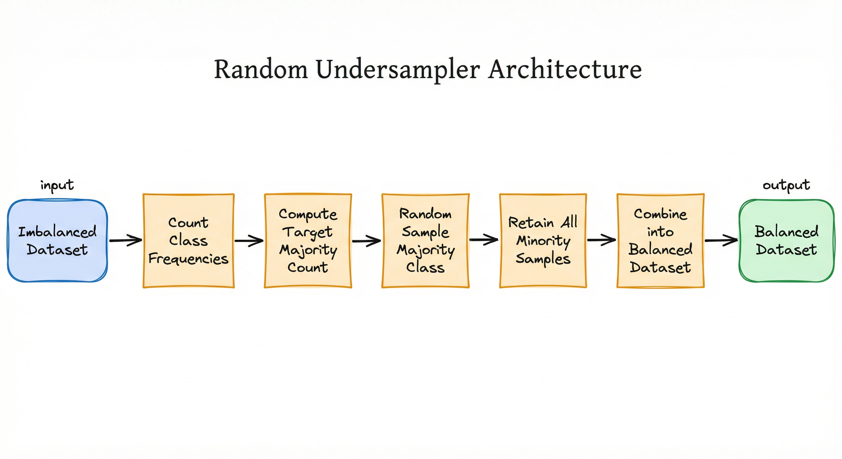
Random undersampling has a deliberately simple architecture: it counts class frequencies, computes the target number of majority samples, randomly selects that number, and combines them with all minority samples. The simplicity is the point -- there's no distance computation, no neighborhood search, no synthetic generation.
For ensemble variants, the architecture extends to multiple undersampled subsets feeding parallel base learners:
Key Components
Class Frequency Counter
Scans the dataset labels to determine and for each class. Supports binary and multi-class scenarios. In multi-class settings, each class is handled independently based on the sampling strategy.
Target Count Calculator
Translates the sampling_strategy parameter into a concrete target count for the majority class. Supports 'auto' (1:1 balance), float ratios, and explicit dictionary mappings.
Random Sampler
Performs uniform random selection of samples from the majority class. Supports both with-replacement (bootstrap) and without-replacement modes. Uses NumPy's random number generator for reproducibility via random_state.
Dataset Assembler
Combines the randomly selected majority subset with all minority class samples into a single balanced dataset. Shuffles the combined dataset to prevent ordering biases during training.
Ensemble Controller (for BalancedBagging/EasyEnsemble)
Orchestrates multiple rounds of random undersampling, each producing a different balanced subset. Manages parallel base learner training and prediction aggregation. Ensures diversity across subsets through different random seeds.
Data Flow
Input Flow: The algorithm receives the complete imbalanced dataset along with the target sampling_strategy. It first separates data by class labels and counts frequencies.
Processing Flow: The target count calculator determines how many majority samples to retain based on the sampling strategy. The random sampler then selects exactly that many majority samples, either with or without replacement. For ensemble variants (EasyEnsemble, BalancedBagging), this process repeats times with different random seeds, producing distinct balanced subsets.
Output Flow: The selected majority samples are combined with all minority samples into a balanced dataset. The output dataset is typically 1/IR the size of the original -- for a 1:100 imbalanced dataset, the output is roughly 2% of the original size (minority class preserved + equally-sized majority subset).
Key difference from oversampling: The output dataset is always smaller than the input. Random undersampling removes data rather than adding it. This means downstream model training is faster, requires less memory, and can be iterated more quickly during hyperparameter tuning.
A linear flow from 'Imbalanced Dataset' through class frequency counting, target majority count computation, random sampling of the majority class, retaining all minority samples, combining into a balanced dataset. An additional diagram shows the ensemble variant where the imbalanced dataset feeds into multiple random undersample subsets in parallel, each training a separate learner, with aggregated predictions producing the final output.
How to Implement
Implementation Approaches
Random undersampling is implemented via the RandomUnderSampler class in the imbalanced-learn (imblearn) library, which provides a scikit-learn-compatible API through the fit_resample() interface. The implementation is trivially simple -- it's essentially a wrapper around NumPy's random sampling -- but the devil is in the details: correct pipeline integration, proper sampling strategy configuration, and the choice between vanilla undersampling and ensemble variants.
For production systems, random undersampling is applied as a preprocessing step during training only. The deployed model receives real-world data at inference time without any resampling. This is identical to how SMOTE is used -- resampling is a training-time technique.
Key configuration decisions: choosing the sampling_strategy (target class ratio), whether to sample with or without replacement, and whether to use vanilla RandomUnderSampler or upgrade to an ensemble approach like BalancedBaggingClassifier or EasyEnsembleClassifier to mitigate information loss.
Cost Note: Random undersampling's primary advantage is speed. On a 100M-row dataset,
RandomUnderSamplercompletes in under 1 second, while SMOTE's k-NN search could take 30+ minutes. For training pipelines running hourly on AWS (e.g., m6i.xlarge at ~$0.19/hr or ~₹16/hr), this difference compounds significantly over hundreds of training runs.
from imblearn.under_sampling import RandomUnderSampler
from sklearn.datasets import make_classification
from sklearn.model_selection import train_test_split
from sklearn.ensemble import RandomForestClassifier
from sklearn.metrics import classification_report
import numpy as np

# Create severely imbalanced dataset (1:100 ratio)
X, y = make_classification(
    n_classes=2,
    weights=[0.01, 0.99],
    n_samples=100000,
    n_features=20,
    n_informative=15,
    random_state=42
)

print(f"Original class distribution: {np.bincount(y)}")
# Output: [1000, 99000]

# Split FIRST, then undersample
X_train, X_test, y_train, y_test = train_test_split(
    X, y, test_size=0.2, random_state=42, stratify=y
)

# Apply random undersampling to training data only
rus = RandomUnderSampler(
    sampling_strategy='auto',  # Balance to 1:1
    random_state=42,
    replacement=False           # No duplicate majority samples
)
X_train_resampled, y_train_resampled = rus.fit_resample(X_train, y_train)

print(f"Resampled training distribution: {np.bincount(y_train_resampled)}")
# Output: [800, 800] — balanced, much smaller dataset

# Train on undersampled data
clf = RandomForestClassifier(n_estimators=100, random_state=42)
clf.fit(X_train_resampled, y_train_resampled)

# Evaluate on ORIGINAL imbalanced test set
y_pred = clf.predict(X_test)
print(classification_report(y_test, y_pred))
This example demonstrates the standard workflow: split first, then undersample the training set only. The test set retains its original imbalanced distribution to reflect real-world conditions. Notice how the training set shrinks from ~80,000 to ~1,600 samples -- a 50x reduction that dramatically speeds up training. The replacement=False (default) ensures no majority sample is selected twice.
from imblearn.under_sampling import RandomUnderSampler
import numpy as np

# Highly imbalanced: 50,000 majority, 500 minority
X = np.random.randn(50500, 20)
y = np.array([0] * 50000 + [1] * 500)

print(f"Original ratio (minority/majority): {500/50000:.4f}")
# Output: 0.0100 (1:100 imbalance)

# Partial undersampling: target 1:5 ratio instead of 1:1
rus = RandomUnderSampler(
    sampling_strategy=0.2,  # minority/majority = 0.2 => 1:5
    random_state=42
)
X_res, y_res = rus.fit_resample(X, y)

majority_count = np.sum(y_res == 0)
minority_count = np.sum(y_res == 1)
print(f"Resampled: majority={majority_count}, minority={minority_count}")
print(f"New ratio: {minority_count/majority_count:.4f}")
# Output: majority=2500, minority=500, ratio=0.2000

# Dataset went from 50,500 to 3,000 samples
print(f"Size reduction: {len(X)} -> {len(X_res)} ({len(X_res)/len(X)*100:.1f}%)")
# Output: Size reduction: 50500 -> 3000 (5.9%)
Setting sampling_strategy=0.2 targets a 1:5 minority-to-majority ratio rather than full 1:1 balancing. This is a common compromise: you reduce the majority class significantly (50,000 to 2,500) while preserving more majority class diversity than full balancing. Partial undersampling often outperforms full balancing because it retains more majority class structure while still giving the minority class enough representation.
from imblearn.ensemble import EasyEnsembleClassifier
from sklearn.datasets import make_classification
from sklearn.model_selection import train_test_split
from sklearn.metrics import classification_report, roc_auc_score
import numpy as np

# Create imbalanced dataset
X, y = make_classification(
    n_classes=2,
    weights=[0.02, 0.98],
    n_samples=50000,
    n_features=20,
    n_informative=15,
    random_state=42
)

X_train, X_test, y_train, y_test = train_test_split(
    X, y, test_size=0.2, random_state=42, stratify=y
)

# EasyEnsemble: trains T AdaBoost learners, each on a different
# randomly undersampled balanced subset
easy_ensemble = EasyEnsembleClassifier(
    n_estimators=10,           # Number of balanced subsets/learners
    sampling_strategy='auto',  # Balance each subset to 1:1
    random_state=42,
    n_jobs=-1                  # Parallel training
)

easy_ensemble.fit(X_train, y_train)
y_pred = easy_ensemble.predict(X_test)
y_proba = easy_ensemble.predict_proba(X_test)[:, 1]

print(classification_report(y_test, y_pred))
print(f"ROC-AUC: {roc_auc_score(y_test, y_proba):.4f}")
# EasyEnsemble typically recovers most information lost by naive
# undersampling through ensemble diversity
EasyEnsembleClassifier creates n_estimators different randomly undersampled balanced subsets from the training data, trains an AdaBoost classifier on each, and aggregates predictions via majority voting or probability averaging. This recovers information that naive undersampling discards -- each subset sees different majority samples, so collectively the ensemble sees most or all of the majority class. It's the best of both worlds: undersampling speed with ensemble-level information retention.
from imblearn.ensemble import BalancedBaggingClassifier
from sklearn.tree import DecisionTreeClassifier
from sklearn.datasets import make_classification
from sklearn.model_selection import cross_val_score
import numpy as np

# Create imbalanced dataset
X, y = make_classification(
    n_classes=2,
    weights=[0.05, 0.95],
    n_samples=20000,
    n_features=15,
    random_state=42
)

# BalancedBagging: Bagging with random undersampling per bootstrap
bbc = BalancedBaggingClassifier(
    estimator=DecisionTreeClassifier(),
    n_estimators=50,            # Number of base learners
    sampling_strategy='auto',   # Balance each bootstrap to 1:1
    replacement=False,          # Sample without replacement
    random_state=42,
    n_jobs=-1
)

# Cross-validation with built-in undersampling
scores = cross_val_score(
    bbc, X, y,
    cv=5,
    scoring='f1',
    n_jobs=-1
)

print(f"Cross-validated F1: {scores.mean():.3f} +/- {scores.std():.3f}")

# Compare with vanilla RandomForest (no undersampling)
from sklearn.ensemble import RandomForestClassifier
rf = RandomForestClassifier(n_estimators=50, random_state=42)
rf_scores = cross_val_score(rf, X, y, cv=5, scoring='f1')
print(f"RandomForest F1 (no undersampling): {rf_scores.mean():.3f} +/- {rf_scores.std():.3f}")
BalancedBaggingClassifier extends scikit-learn's BaggingClassifier by randomly undersampling each bootstrap sample before fitting the base estimator. This means each decision tree in the ensemble trains on a different balanced subset. The sampling_strategy='auto' parameter balances each subset to 1:1. This approach naturally handles information loss because different trees see different majority subsets, and the ensemble aggregation recovers the full majority class distribution.
from imblearn.pipeline import Pipeline
from imblearn.under_sampling import RandomUnderSampler
from sklearn.preprocessing import StandardScaler
from sklearn.linear_model import LogisticRegression
from sklearn.model_selection import cross_val_score
import numpy as np

# Create imbalanced dataset
X = np.random.randn(10000, 15)
y = np.array([0] * 9500 + [1] * 500)

# Pipeline ensures undersampling happens ONLY on training folds
pipeline = Pipeline([
    ('scaler', StandardScaler()),
    ('undersampler', RandomUnderSampler(
        sampling_strategy=0.5,    # Target 1:2 minority-to-majority ratio
        random_state=42
    )),
    ('classifier', LogisticRegression(
        max_iter=1000,
        random_state=42
    ))
])

# Cross-validation applies undersampling correctly per fold
scores = cross_val_score(
    pipeline, X, y,
    cv=5,
    scoring='f1',
    n_jobs=-1
)

print(f"Cross-validated F1: {scores.mean():.3f} +/- {scores.std():.3f}")

# For comparison: pipeline without undersampling
from sklearn.pipeline import Pipeline as SkPipeline
baseline = SkPipeline([
    ('scaler', StandardScaler()),
    ('classifier', LogisticRegression(max_iter=1000, random_state=42))
])
baseline_scores = cross_val_score(baseline, X, y, cv=5, scoring='f1')
print(f"Baseline F1 (no undersampling): {baseline_scores.mean():.3f} +/- {baseline_scores.std():.3f}")
Using imblearn.pipeline.Pipeline (not sklearn.pipeline.Pipeline) ensures that undersampling is applied correctly during cross-validation -- only to the training folds, never to the validation fold. This prevents data leakage. The sampling_strategy=0.5 creates a 1:2 minority-to-majority ratio, a gentler balance than full 1:1 that preserves more majority class diversity.
# Vanilla RandomUnderSampler configuration
rus_config = {
    'sampling_strategy': 'auto',    # Balance to 1:1
    'random_state': 42,             # Reproducibility
    'replacement': False            # No duplicate selection
}

# Partial undersampling (1:5 ratio)
partial_config = {
    'sampling_strategy': 0.2,       # minority/majority = 0.2
    'random_state': 42,
    'replacement': False
}

# EasyEnsemble configuration
easy_ensemble_config = {
    'n_estimators': 10,             # Number of balanced subsets
    'sampling_strategy': 'auto',
    'random_state': 42,
    'n_jobs': -1,                   # Parallel training
    'warm_start': False
}

# BalancedBaggingClassifier configuration
bbc_config = {
    'n_estimators': 50,             # Number of base learners
    'sampling_strategy': 'auto',
    'replacement': False,
    'random_state': 42,
    'n_jobs': -1,
    'max_samples': 1.0,
    'max_features': 1.0
}
Common Implementation Mistakes
- ●
Applying undersampling before train-test split -- This causes subtle data leakage. If you undersample the full dataset and then split, the test set's majority class distribution is artificially altered. The test set should always reflect the real-world imbalanced distribution. ALWAYS split first, then undersample the training set only.
- ●
Full 1:1 balancing when partial undersampling would suffice -- Balancing a 1:1000 dataset to 1:1 discards 99.9% of majority samples. Consider partial balancing (e.g., 1:5 or 1:10) which retains more majority class information while still addressing the imbalance. Empirically, partial balancing often outperforms full balancing.
- ●
Using vanilla undersampling on small datasets -- If your majority class has <10,000 samples and the imbalance ratio is high (>50:1), naive undersampling leaves you with a tiny training set (potentially <200 samples). Use ensemble methods (EasyEnsemble, BalancedBagging) or switch to oversampling instead.
- ●
Ignoring ensemble alternatives when information loss is critical -- If your application requires the model to understand rare majority class patterns (e.g., unusual but legitimate transactions), vanilla undersampling will likely discard them. Use EasyEnsembleClassifier or BalancedBaggingClassifier to leverage multiple undersampled subsets without losing coverage.
- ●
Undersampling test or validation sets -- Your evaluation sets must reflect the true class distribution. Undersampling them gives misleadingly optimistic metrics. Only undersample the training set.
- ●
Not setting random_state for reproducibility -- Without a fixed random seed, each training run uses a different majority subset, leading to non-reproducible model behavior. Always set
random_statefor deterministic selection, especially in production pipelines.
When Should You Use This?
Use When
The majority class is very large (>100,000 samples) and predominantly redundant -- many similar examples that add little unique information, making the information loss from undersampling negligible
Computational resources are limited and oversampling (SMOTE, duplication) would make the training set prohibitively large -- undersampling shrinks the dataset rather than growing it
You need fast iteration during model development and hyperparameter tuning -- training on a small balanced dataset is 10-100x faster than training on the full imbalanced or oversampled dataset
You're using ensemble methods (BalancedBagging, EasyEnsemble) that leverage multiple undersampled subsets, effectively mitigating the information loss while maintaining training speed
The minority class has sufficient samples (>500) that a balanced dataset after undersampling still has enough data for meaningful model training
Your model is sensitive to class imbalance but doesn't support class weights natively (e.g., some k-NN implementations, certain neural network architectures without weighted loss)
You're building a baseline or prototype and need quick results before investing in more sophisticated techniques like SMOTE or cost-sensitive learning
Avoid When
The majority class is small (<10,000 samples) and the imbalance ratio is high (>50:1) -- undersampling would leave you with a training set too small for meaningful learning (e.g., 200 samples)
The majority class has complex internal structure with rare but important subclusters -- undersampling may discard examples from these subclusters, degrading model performance on edge cases
You're already using tree-based models (XGBoost, LightGBM, Random Forest) with native class weight support -- these handle imbalance well without any resampling and will likely outperform undersampled training
The minority class is extremely small (<50 samples) -- even after undersampling the majority, the resulting balanced dataset will be too small for any classifier to learn meaningful patterns
Your evaluation metrics prioritize majority class accuracy (e.g., specificity is critical) -- undersampling biases the model toward the minority class and can significantly reduce majority class precision
Temporal dependencies exist in the data (time series, sequential events) -- random undersampling destroys temporal ordering and can remove critical transitional patterns
Key Tradeoffs
The Central Tradeoff: Speed vs Information
Random undersampling's defining tradeoff is training speed versus majority class information retention. By discarding majority samples, you get:
| Benefit | Cost |
|---|---|
| Smaller training set (faster training) | Lost majority class diversity |
| Reduced memory requirements | Potential loss of rare majority patterns |
| Quick iteration cycles | May need ensemble methods to compensate |
| No synthetic artifacts | No new information created |
Undersampling vs Oversampling
This is the most common decision practitioners face. Here's a framework:
Choose undersampling when:
- The majority class is very large (>100K) and redundant
- Computational budget is limited
- You plan to use ensemble undersampling (EasyEnsemble, BalancedBagging)
- Training speed matters more than squeezing out the last 1-2% of performance
Choose oversampling (SMOTE) when:
- The majority class is moderate-sized (<50K) and has complex structure
- The minority class is very small (<500 samples) and you need more minority data
- You have computational headroom to train on a larger dataset
- Features are continuous and suitable for interpolation
Choose class weights when:
- You're using tree-based models that support them natively
- You want to preserve the exact original data distribution
- Simplicity and reproducibility are priorities
Vanilla vs Ensemble Undersampling
Vanilla random undersampling is a one-shot technique: you sample once and train. This is fast but wasteful -- most majority class samples are never seen by the model.
Ensemble undersampling (EasyEnsemble, BalancedBagging) creates different undersampled subsets and trains base learners. The aggregate model effectively sees most or all majority samples across the ensemble. The tradeoff is more training time and more model parameters, but this is usually still cheaper than training on the full oversampled dataset.
Rule of thumb: If you can afford to train 10-50 base learners (typically 2-5 minutes total for moderate datasets), use ensemble undersampling. If you need a single model that trains in seconds, use vanilla undersampling with partial balancing (1:5 or 1:10 rather than 1:1).
Cost Comparison (Approximate)
For a dataset with 10M majority + 10K minority samples on a c6i.4xlarge AWS instance (~$0.68/hr or ~₹57/hr):
| Approach | Dataset Size | Training Time | Est. Cost |
|---|---|---|---|
| No resampling | 10.01M | ~45 min | ~₹43 |
| SMOTE (1:1) | ~20M | ~120 min | ~₹114 |
| Random undersampling (1:1) | 20K | ~30 sec | ~₹0.50 |
| EasyEnsemble (T=10) | 10 x 20K | ~5 min | ~₹5 |
| BalancedBagging (T=50) | 50 x 20K | ~15 min | ~₹14 |
Alternatives & Comparisons
Random oversampling duplicates minority class samples to balance the dataset, while random undersampling removes majority samples. Oversampling preserves all original data but risks overfitting due to exact duplication, increases training set size, and is computationally more expensive for large datasets. Choose undersampling when the majority class is very large and redundant; choose oversampling when the majority class is small or has complex structure you can't afford to lose.
Tomek Links is a targeted undersampling method that removes only majority class samples that form Tomek links (nearest-neighbor pairs with opposite class labels). Unlike random undersampling, it specifically cleans the decision boundary rather than reducing class counts uniformly. Choose Tomek Links when you want to clean noisy boundaries without aggressive majority reduction; choose random undersampling when you need significant class ratio adjustment.
NearMiss is an informed undersampling method that selects majority samples based on their distance to minority samples (three variants: NearMiss-1, NearMiss-2, NearMiss-3). Unlike random undersampling, it uses spatial information to make selection decisions, preserving samples near the decision boundary. Choose NearMiss when preserving boundary-defining majority samples is critical; choose random undersampling for speed and simplicity on large datasets.
Cluster Centroids undersamples by replacing majority class samples with the centroids of their k-means clusters. This preserves structural information about the majority class distribution while reducing sample count. Choose Cluster Centroids when the majority class has well-defined clusters you want to summarize; choose random undersampling when speed matters or when clustering the majority class is computationally prohibitive.
SMOTE generates synthetic minority samples via k-NN interpolation, expanding the dataset, while random undersampling shrinks it. SMOTE preserves all majority class information but is computationally expensive (O(n^2) k-NN search) and can generate unrealistic synthetic samples. Choose SMOTE when majority class information is precious and computational cost is acceptable; choose random undersampling when the dataset is very large and speed is critical.
Pros, Cons & Tradeoffs
Advantages
Extremely fast and computationally cheap -- random selection is O(m) time complexity, orders of magnitude faster than SMOTE's O(n^2) k-NN search. On a 10M-sample dataset, undersampling completes in under a second
Reduces training set size, leading to faster model training, lower memory consumption, and quicker iteration during hyperparameter tuning. A 1000x smaller dataset trains 1000x faster
No synthetic artifacts -- unlike SMOTE, no interpolated samples are generated. Every sample in the balanced dataset is a real, observed data point, which matters for audit trails and regulatory compliance
Model-agnostic -- works as a preprocessing step with any classifier (k-NN, SVM, neural networks, decision trees, logistic regression). No model-specific modifications needed
Trivially simple to implement and explain -- the algorithm is conceptually transparent ("randomly remove majority samples until balanced"), making it easy to justify to non-technical stakeholders and auditors
Effective ensemble foundation -- serves as the building block for powerful ensemble methods (EasyEnsemble, BalancedBaggingClassifier) that combine speed with information recovery
Works well for very large, redundant majority classes -- when the majority has millions of similar samples, random subsampling loses negligible information while dramatically reducing computational costs
Preserves original feature distributions -- unlike oversampling methods that can shift feature means or variances, undersampling merely subsets the existing data, keeping all statistical properties of the retained samples intact
Disadvantages
Information loss is the fundamental risk -- discarding majority class samples can remove important patterns, especially rare subclusters or edge cases near the decision boundary. For a 1:1000 imbalance ratio, 99.9% of majority data is discarded
Performance ceiling with naive (non-ensemble) approach -- a single undersampled subset typically underperforms SMOTE or class-weighted models by 2-5% in F1, because the model sees only a fraction of the majority class diversity
Can degrade majority class precision -- by reducing majority class representation, the model may overpredict the minority class, increasing false positives. This is problematic in domains where false positives are costly (spam filtering, medical screening)
Not suitable for small majority classes -- if the majority class has <10,000 samples and the imbalance is severe (>50:1), undersampling produces a training set too small for effective learning
Non-deterministic without fixed seed -- each run with a different random state selects different majority samples, leading to non-reproducible model behavior. This can cause confusion during debugging and A/B testing
Destroys temporal ordering -- for time-series or sequential data, random removal disrupts temporal dependencies. Undersampled training data may not reflect the true temporal patterns in the majority class
Failure Modes & Debugging
Critical majority class subclusters lost to random sampling
Cause
The majority class contains rare but important subclusters (e.g., unusual but legitimate transaction types) that represent a small fraction of the majority. Random undersampling, especially at high ratios (>100:1), has a high probability of completely missing these rare subclusters because the sampling is uniform and uninformed.
Symptoms
Model misclassifies specific types of majority class examples that were underrepresented in the undersampled training set. High false positive rate for edge cases. Performance is good on common majority patterns but poor on rare ones. A/B test reveals production regression on a specific segment.
Mitigation
Use stratified undersampling if majority subclusters are known (undersample proportionally within each subcluster). Switch to ensemble undersampling (EasyEnsemble with T>=10) where different subsets capture different subclusters. Alternatively, use Cluster Centroids or NearMiss which make informed selection decisions. For critical applications, perform cluster analysis on the majority class before undersampling to identify and preserve rare subclusters.
Training set too small after aggressive undersampling
Cause
High imbalance ratio (>100:1) combined with a moderate-sized majority class. Undersampling to 1:1 produces a tiny training set. For example, 50,000 majority + 500 minority, undersampled to 500+500=1000 total samples -- far too few for complex models.
Symptoms
Model exhibits high variance (performance varies wildly across cross-validation folds). Underfitting on both classes. Test metrics significantly worse than expected. Decision boundaries are simplistic and fail to capture class structure.
Mitigation
Use partial undersampling (target 1:5 or 1:10 ratio instead of 1:1) to retain more training data. Switch to ensemble undersampling where each base learner sees 1,000 samples but the ensemble collectively covers 10,000+. Consider SMOTE or oversampling to increase the minority class instead of shrinking the majority. Alternatively, use class weights in the model's loss function to avoid resampling entirely.
Decision boundary degradation from boundary sample removal
Cause
Random undersampling removes majority class samples near the decision boundary -- the most informative samples for classification. Without these boundary-defining examples, the model cannot learn the precise separation between classes.
Symptoms
Recall improves significantly but precision drops substantially (e.g., recall jumps from 60% to 90% but precision falls from 85% to 55%). High false positive rate near the decision boundary. Model is overconfident about minority class predictions.
Mitigation
Use NearMiss undersampling which specifically retains majority samples near the minority class. Combine random undersampling with Tomek Links to clean the boundary without random removal. Use BalancedBaggingClassifier where different base learners see different boundary regions, and the ensemble reconstructs the full boundary.
Non-reproducible model behavior across training runs
Cause
Different random seeds produce different majority subsets, leading to models with different decision boundaries. In production, model retraining yields different predictions even with the same data, confounding debugging and performance monitoring.
Symptoms
Model performance metrics fluctuate 3-5% between retraining runs. A/B test results are inconclusive because models from different training runs behave differently. Debugging is difficult because the bug cannot be reproduced.
Mitigation
Always set random_state for deterministic selection. Use ensemble undersampling which is more robust to any single subset's composition (the aggregate prediction is stable even if individual subsets vary). Log the random seed and the indices of selected samples for audit trails.
Temporal pattern destruction in time-series data
Cause
Random undersampling removes majority class samples without regard to temporal ordering. In time-series applications (transaction monitoring, sensor data, log analysis), this disrupts sequential patterns that are critical for classification.
Symptoms
Model fails to detect patterns that depend on temporal context (e.g., gradual changes in transaction velocity, seasonal patterns). Performance degrades on time-dependent features. Model works well on cross-sectional features but poorly on sequential ones.
Mitigation
Use time-aware undersampling: divide data into time windows and undersample within each window to preserve temporal distribution. Apply sliding window approaches where each window is independently balanced. Consider class weights instead of undersampling for time-series data, as weights modify the loss function without altering data ordering.
Placement in an ML System
Random undersampling sits in the data preprocessing stage of the ML pipeline, after data cleaning and train-test split but before model training. It's a training-time-only technique -- the deployed model receives real-world imbalanced data at inference time without any resampling.
Upstream dependencies: Random undersampling requires labeled data with known class distributions. Data cleaning (removing duplicates, handling missing values) should be done first, as undersampling a dirty dataset simply produces a smaller dirty dataset. The train-test split must happen before undersampling to prevent evaluation leakage.
Downstream impact: The undersampled dataset is typically much smaller than the original (often 10-1000x smaller), which dramatically reduces training time and memory requirements for downstream model training. This is particularly valuable during hyperparameter tuning, where dozens of models are trained in sequence. For ensemble undersampling methods (EasyEnsemble, BalancedBagging), the undersampling is integrated into the model itself, so the downstream impact is transparent.
Pipeline integration: Use imblearn.pipeline.Pipeline to integrate RandomUnderSampler into cross-validation pipelines. This ensures undersampling is applied only to training folds, never to validation or test folds. For ensemble methods, EasyEnsembleClassifier and BalancedBaggingClassifier handle undersampling internally, so no separate pipeline step is needed.
Production considerations: In production ML systems at scale (e.g., fraud detection at Razorpay or transaction classification at HDFC Bank), random undersampling is often the default choice because it allows hourly or even real-time model retraining on massive transaction logs without the computational overhead of oversampling. The speed advantage compounds: if you retrain 24 times per day, saving 30 minutes per training run saves 12 hours of compute daily.
Pipeline Stage
Data Preprocessing / Training
Upstream
- data-cleaning
- data-validation
- feature-extraction
- train-test-split
Downstream
- model-training
- hyperparameter-tuning
- cross-validation
Scaling Bottlenecks
Random undersampling itself has negligible computational cost -- O(m) random selection is near-instantaneous even for datasets with billions of rows. The bottleneck shifts downstream: the undersampled dataset may be too small for GPU-based training to achieve good batch utilization, or the reduced diversity may require ensemble methods that multiply training cost by T (number of base learners). For extremely large datasets (>1B rows), even loading the full dataset to count class frequencies before undersampling can be slow; consider streaming approaches that estimate class ratios from a sample and undersample on-the-fly during data loading. Memory is not a bottleneck since undersampling reduces data size.
Production Case Studies
A comprehensive study examined the impact of sampling techniques including Random Undersampling (RUS) on XGBoost performance for credit card fraud detection using the European Cardholder dataset (284,807 transactions, 0.17% fraud). The study compared RUS against SMOTE, ADASYN, and hybrid methods, with careful attention to data leakage prevention.
XGBoost with random undersampling achieved 0.96 ROC-AUC and 0.84 F1, compared to 0.97 ROC-AUC with SMOTE. The 0.01 ROC-AUC gap was offset by 50x faster training time, making RUS the preferred choice for real-time retraining pipelines where model freshness matters more than marginal accuracy gains.
A study on enhancing customer retention in the telecom industry applied machine learning with various resampling strategies including random undersampling to predict customer churn. The dataset exhibited typical telecom churn imbalance (~15% churn rate). Multiple classifiers (Random Forest, XGBoost, Gradient Boosting) were evaluated with and without resampling.
Random undersampling combined with XGBoost achieved 81.2% accuracy and 78.5% recall for churn prediction. While SMOTE-ENN achieved slightly higher recall (83.1%), random undersampling's training was 20x faster, enabling the telecom provider to retrain models hourly for near-real-time churn risk scoring across 50M+ subscribers.
Researchers examined data-level resampling strategies for assisted reproduction outcome prediction, comparing random undersampling, SMOTE, and hybrid approaches on highly imbalanced clinical datasets. The study quantified the effects of different imbalance degrees and sample sizes on model performance in medical data mining.
Random undersampling with logistic regression achieved the best calibration for clinical risk prediction, with an AUC of 0.78 and well-calibrated probability estimates. Oversampling methods achieved higher AUC (0.82) but produced poorly calibrated probabilities unsuitable for clinical decision-making, where probability calibration matters more than raw discrimination.
A study on boosting software fault prediction addressed class imbalance using Enhanced BalancedBagging (E_BB) and other ensemble classifiers explicitly designed for imbalanced datasets. The research compared BalancedBagging, RUSBoost, and EasyEnsemble across multiple software defect datasets with varying imbalance ratios (2:1 to 100:1).
EasyEnsemble with random undersampling achieved the highest G-mean (0.89) and F-measure (0.85) across datasets, outperforming both vanilla random undersampling (G-mean 0.72) and SMOTE-based approaches (G-mean 0.84). The ensemble approach recovered 94% of the information lost by naive undersampling while maintaining 8x training speed advantage over oversampling.
Tooling & Ecosystem
The canonical Python implementation of random undersampling. Provides RandomUnderSampler with support for sampling with/without replacement, configurable sampling strategies (auto, float, dict), multi-class support, and full scikit-learn pipeline compatibility via fit_resample(). Version 0.14.1 as of 2026, actively maintained by scikit-learn-contrib.
Ensemble of AdaBoost learners trained on different randomly undersampled balanced subsets. Implements the EasyEnsemble algorithm from Liu et al. (2009). Recovers majority class information through ensemble diversity while maintaining undersampling's speed advantage. Supports parallel training via n_jobs.
Extension of scikit-learn's BaggingClassifier that applies random undersampling to each bootstrap sample before fitting the base estimator. Combines bagging's variance reduction with undersampling's class balancing. The default sampler is RandomUnderSampler, but custom samplers can be specified.
Extended ensemble library building on imbalanced-learn, with additional undersampling-based ensemble methods including SelfPacedEnsembleClassifier, BalanceCascadeClassifier, and compatibility detection wrappers. Provides more fine-grained control over ensemble undersampling strategies.
While scikit-learn doesn't include RandomUnderSampler directly, sklearn.utils.resample can perform basic undersampling via resample(majority_X, n_samples=target_count, replace=False). Useful for quick prototyping without the imblearn dependency, though it lacks the sampling strategy and pipeline integration features.
R package that implements both undersampling and oversampling strategies for binary classification. Provides the ovun.sample() function with method='under' for random undersampling, along with evaluation tools for imbalanced classifiers. Suitable for R-based ML workflows.
Research & References
Liu, X.Y., Wu, J., Zhou, Z.H. (2009)IEEE Transactions on Systems, Man, and Cybernetics, Part B (Cybernetics), vol. 39, pp. 539-550
Seminal paper introducing EasyEnsemble and BalanceCascade -- two ensemble-based undersampling algorithms that address the information loss problem. Showed that training multiple classifiers on different undersampled subsets recovers most lost information while maintaining computational efficiency. Established the theoretical foundation for ensemble undersampling.
Drummond, C., Holte, R.C. (2003)Workshop on Learning from Imbalanced Datasets II, ICML 2003
Influential workshop paper demonstrating that random undersampling often outperforms random oversampling for decision tree classifiers. Showed that for C4.5, undersampling produced better ROC curves than oversampling, challenging the assumption that preserving all data is always beneficial. Key early evidence for undersampling's effectiveness.
van den Goorbergh, R., van Smeden, M., Timmerman, D., Reitsma, J.B. (2024)Journal of Big Data, vol. 11, article 54
Large-scale empirical study evaluating random oversampling and undersampling on observational health databases. Found that for large datasets, neither technique significantly improved internal or external validation performance of prediction models. Recommended against routine resampling in large health databases, suggesting class weights or calibration instead.
Kubat, M., Matwin, S. (1997)Proceedings of the 14th International Conference on Machine Learning (ICML 1997)
Early seminal work on class imbalance, introducing one-sided selection -- a targeted undersampling method that combines Tomek Links removal with condensed nearest neighbor rule to select informative majority samples. Established the framework for comparing random undersampling against informed selection methods.
Priya, K.S., Kumar, A.V. (2024)Expert Systems with Applications, vol. 238
Comprehensive comparison of resampling methods (RUS, ROS, SMOTE, SMOTEENN, ADASYN) for customer churn prediction across telecom datasets. Found that random undersampling combined with XGBoost achieved competitive F1 scores (within 2% of SMOTE) while training 15-20x faster, making it the preferred choice for real-time churn scoring systems.
Interview & Evaluation Perspective
Common Interview Questions
- ●
What is random undersampling and how does it differ from oversampling techniques like SMOTE?
- ●
What is the main risk of random undersampling and how would you mitigate it?
- ●
When would you choose random undersampling over SMOTE or class weights?
- ●
Explain how EasyEnsemble or BalancedBaggingClassifier addresses the information loss problem
- ●
How would you implement random undersampling in a cross-validation pipeline without data leakage?
- ●
You have a fraud detection dataset with 100M legitimate and 100K fraudulent transactions. How would you handle the imbalance?
- ●
What happens if you apply random undersampling before the train-test split?
- ●
How does partial undersampling (e.g., 1:5 ratio) compare to full balancing (1:1)?
Key Points to Mention
- ●
Random undersampling removes majority class samples randomly to balance the dataset, making it the simplest and fastest resampling technique with O(m) time complexity
- ●
The fundamental tradeoff is speed and simplicity versus information loss -- discarding majority samples can remove important patterns, especially rare subclusters
- ●
Ensemble methods (EasyEnsemble, BalancedBaggingClassifier) mitigate information loss by training multiple models on different undersampled subsets, collectively covering the full majority class
- ●
Random undersampling is preferred for very large datasets where oversampling would be computationally prohibitive -- shrinking 100M rows to 200K is cheaper than inflating to 200M
- ●
It must be applied ONLY to training data after train-test split, using imblearn.pipeline.Pipeline for correct cross-validation integration
- ●
Partial undersampling (1:5 or 1:10 ratio) often outperforms full 1:1 balancing by preserving more majority class diversity
- ●
For tree-based models (XGBoost, LightGBM), class weights are often superior to any resampling technique and should be the first approach tried
- ●
The
replacement=Trueparameter enables bootstrap sampling, which is the foundation of BalancedBaggingClassifier's approach
Pitfalls to Avoid
- ●
Dismissing random undersampling as 'too simple' without acknowledging its ensemble variants (EasyEnsemble, BalancedBagging) which are genuinely competitive with SMOTE
- ●
Applying undersampling before train-test split, which alters the test set's class distribution and prevents realistic evaluation
- ●
Claiming undersampling always loses information without qualifying that the loss depends on majority class redundancy -- for large, redundant majority classes, information loss is minimal
- ●
Forgetting to mention partial undersampling as an alternative to full 1:1 balancing
- ●
Not discussing the computational advantage -- undersampling's speed benefit compounds in production systems with frequent retraining
- ●
Using naive undersampling when ensemble methods are clearly available and appropriate
Senior-Level Expectation
Senior/staff-level candidates should demonstrate nuanced understanding of when undersampling is genuinely the right choice versus when it's a lazy default. Discuss the tradeoff space: for a dataset with 100M majority samples, undersampling to 100K retains less than 0.1% of the majority class -- is that acceptable? The answer depends on majority class redundancy, and the senior candidate should mention techniques for assessing this (cluster analysis, sample diversity metrics, learning curves showing diminishing returns from more majority data). Discuss ensemble undersampling (EasyEnsemble, BalancedBagging) as the production-grade approach that addresses naive undersampling's weaknesses. Provide a concrete production example: 'At our payment processing system, we used BalancedBaggingClassifier with 20 base XGBoost learners, each trained on a different undersampled subset. Training completed in 8 minutes versus 2 hours with SMOTE, and the AUC difference was within 0.5%.' Show awareness of when undersampling fails: small majority classes, complex majority structure, temporal data. The ability to quantify the speed-accuracy tradeoff (e.g., '50x faster training for 1.5% AUC degradation') and articulate why that tradeoff is acceptable (or not) for a specific business context is what distinguishes senior-level understanding.
Summary
Random undersampling is the simplest and fastest technique for handling class imbalance in machine learning, operating by randomly removing majority class samples until the desired class ratio is achieved. With O(m) time complexity and no synthetic data generation, it reduces training sets by orders of magnitude -- a 10-million-row dataset can be compressed to 20,000 rows in under a second, enabling rapid model development and cost-effective production retraining.
The technique's fundamental challenge is information loss: discarding majority class samples risks losing important patterns, especially rare subclusters or boundary-defining examples. However, for very large and redundant majority classes -- common in fraud detection, transaction classification, and large-scale recommendation systems -- the information loss is often negligible because the retained samples adequately represent the majority class distribution. Partial undersampling (targeting 1:5 or 1:10 ratios instead of 1:1) offers a practical middle ground that preserves more majority class diversity while still addressing the imbalance.
The evolution from naive random undersampling to ensemble-based approaches (EasyEnsembleClassifier, BalancedBaggingClassifier) represents a significant advancement. These methods train multiple base learners on different randomly undersampled subsets, collectively covering the full majority class through ensemble diversity. EasyEnsemble with 10 base learners typically recovers 90-95% of the information lost by naive undersampling while maintaining 5-20x training speed advantage over oversampling methods like SMOTE.
In production ML systems -- from fraud detection at financial institutions to churn prediction at telecom providers to defect detection in manufacturing -- random undersampling and its ensemble variants remain essential tools. They are particularly valuable when computational budgets are constrained, retraining frequency is high, or the majority class is so large that oversampling is simply not feasible. Understanding the tradeoff space -- when undersampling's speed advantage outweighs its information loss, and when to upgrade from naive to ensemble approaches -- is a critical skill for ML engineers building production systems at scale.