Random Oversampler in Machine Learning
Random oversampling is the simplest and oldest technique for handling class imbalance in machine learning. The core idea could not be more straightforward: you take the minority class samples and duplicate them -- randomly, with replacement -- until the class distribution is balanced. No interpolation, no synthetic generation, no nearest neighbor searches. Just copies.
But don't mistake simplicity for ineffectiveness. Random oversampling remains one of the most widely used resampling techniques in production ML systems, from fraud detection pipelines at Razorpay to churn prediction models at Jio. It is the baseline that every more sophisticated technique (SMOTE, ADASYN, Borderline-SMOTE) is compared against, and in a surprising number of real-world scenarios, it performs just as well or better than its fancier counterparts.
The technique has evolved since its naive form. Modern implementations in imbalanced-learn support a shrinkage parameter that enables smoothed bootstrap sampling -- also known as ROSE (Random Over-Sampling Examples) -- which adds controlled Gaussian perturbation to duplicated samples rather than creating exact copies. This single extension transforms random oversampling from a blunt instrument into a nuanced tool that can mitigate overfitting while preserving the simplicity advantage.
Understanding when random oversampling works, when it fails, and when to reach for alternatives is a core competency for any ML engineer working with imbalanced data -- which, in practice, means almost every ML engineer.
Concept Snapshot
- What It Is
- A data-level resampling technique that balances class distributions by duplicating minority class samples (with or without small random perturbations), enabling classifiers to learn from underrepresented classes.
- Category
- Data Generation
- Complexity
- Beginner
- Inputs / Outputs
- Inputs: imbalanced training dataset where minority class is underrepresented. Outputs: balanced dataset where minority class samples have been duplicated (or perturbed copies created) to match the target class ratio.
- System Placement
- Applied during the data preprocessing phase, after train-test split and before model training. Never applied to validation or test sets.
- Also Known As
- Random Over-Sampling (ROS), Naive oversampling, Duplication oversampling, Bootstrap oversampling, ROSE (when using smoothed bootstrap)
- Typical Users
- ML engineers, Data scientists, Applied researchers, ML platform engineers, Kaggle competitors
- Prerequisites
- Class imbalance concepts, Train-test split methodology, Precision-recall tradeoffs, Bootstrap sampling basics
- Key Terms
- class imbalanceoversamplingwith replacementminority classmajority classshrinkagesmoothed bootstrapROSEsampling_strategyimbalanced-learn
Why This Concept Exists
The Class Imbalance Problem
Real-world datasets are almost never balanced. Fraudulent transactions might represent 0.1% of all payment activity at PhonePe. Manufacturing defects occur in 0.5% of products on a Tata Motors assembly line. Rare cancers appear in fewer than 1 in 10,000 medical scans. In each case, the class you care about most -- the minority -- is massively outnumbered.
Standard ML algorithms optimize for overall accuracy. A fraud detector that always predicts "legitimate" achieves 99.9% accuracy on a 1000:1 imbalanced dataset while catching exactly zero frauds. The model learned the optimal shortcut: ignore the minority entirely.
The Simplest Fix: Just Copy the Minority
Random oversampling is the most intuitive response to this problem. If the model ignores the minority class because there aren't enough samples, give it more. How? Pick minority samples at random (with replacement) and duplicate them until you reach the desired class ratio.
This approach predates all the sophisticated techniques. Before Chawla et al. introduced SMOTE in 2002, random oversampling was the primary data-level strategy for addressing class imbalance. He and Garcia's influential 2009 IEEE TKDE survey, Learning from Imbalanced Data, identifies random oversampling as one of the foundational resampling methods alongside random undersampling.
Why It Persists Despite Known Limitations
You might expect that SMOTE and its variants would have replaced random oversampling entirely. They haven't, for several reasons:
Simplicity: Random oversampling has zero hyperparameters in its basic form (no k-neighbors to tune) and is trivially parallelizable. In a production pipeline with 50+ components, simplicity compounds.
Speed: No k-NN search means computational cost instead of or . For datasets with millions of minority samples, this difference matters enormously.
Universality: Random oversampling works with any data type -- tabular, text embeddings, image features, categorical, mixed. SMOTE requires a meaningful distance metric and continuous features. When your features include sparse text embeddings and categorical flags, random oversampling just works.
Competitive performance: Multiple empirical studies have shown that random oversampling performs comparably to SMOTE on many real-world benchmarks, particularly when paired with regularized models (tree ensembles, L2-regularized logistic regression) that naturally resist overfitting from duplicated samples.
Historical Note: The ROSE (Random Over-Sampling Examples) extension, proposed by Menardi and Torelli in 2014, added smoothed bootstrap to random oversampling -- creating perturbed copies rather than exact duplicates. This was integrated into
imbalanced-learnas theshrinkageparameter, effectively modernizing the oldest oversampling technique.
Core Intuition & Mental Model
The Core Idea: More Copies, More Attention
Think of it this way: you're training a model that processes examples one by one (or in mini-batches). If class A has 10,000 samples and class B has 100 samples, class A's patterns get reinforced 100x more often during training. The model's parameters drift heavily toward predicting class A because that's where the gradient signal overwhelmingly comes from.
Random oversampling fixes the imbalance at the data level. By duplicating class B's 100 samples until you have 10,000, each class now contributes equally to the training signal. The model can no longer take the shortcut of ignoring class B.
The Library Analogy
Imagine a library where 99 shelves contain Hindi novels and 1 shelf contains Urdu poetry. If a student randomly browses shelves, they'll almost never encounter Urdu poetry. Random oversampling is equivalent to photocopying the Urdu poetry collection and placing copies on 98 additional shelves. Now the student encounters both genres equally often.
The limitation is obvious: the student sees the same poems over and over. They might memorize specific poems rather than learning what makes Urdu poetry distinctive in general. This is the overfitting risk of naive random oversampling.
The Smoothed Bootstrap Extension
Here's where the ROSE (smoothed bootstrap) idea gets clever. Instead of making exact photocopies, imagine a slightly imperfect photocopier that introduces tiny random smudges. Each copy is slightly different from the original -- not a new poem, but not an identical reproduction either.
Mathematically, the smoothed bootstrap draws a sample from the original minority class, then adds a small Gaussian perturbation controlled by the shrinkage parameter. Higher shrinkage means more perturbation (blurrier copies), while shrinkage of 0 means exact duplication (perfect copies). This small modification can significantly reduce overfitting while maintaining the simplicity of the random oversampling framework.
What Random Oversampling Does NOT Do
This is important to internalize: random oversampling does not create new information. Whether you're duplicating exactly or perturbing slightly, the synthetic samples don't reveal patterns that weren't already present in the original data. If your 100 minority samples are noisy, mislabeled, or unrepresentative, oversampling amplifies those problems.
The technique assumes your original minority samples are reasonably representative of the true minority distribution. If they're not, no amount of duplication or perturbation will fix that -- you need better data collection.
Expert Insight: Random oversampling is equivalent to adjusting class weights in the loss function when training with SGD. Both approaches increase the effective contribution of minority samples to gradient updates. The practical difference is that oversampling changes the data, while class weights change the optimization -- but the mathematical effect on expected gradients is identical for exact duplication.
Technical Foundations
Mathematical Formulation
Let be a training set with , where class 1 (minority) has samples and class 0 (majority) has samples, with imbalance ratio .
Naive Random Oversampling
To produce a balanced dataset, generate additional minority samples by sampling uniformly at random with replacement from the existing minority set :
The resampled dataset is where , yielding a balanced class distribution.
Smoothed Bootstrap (ROSE)
The smoothed variant, proposed by Menardi and Torelli (2014), adds a Gaussian perturbation to each drawn sample:
where:
- is a randomly selected minority sample
- is the shrinkage factor (scalar controlling perturbation magnitude)
- is the estimated covariance matrix of class
The covariance matrix is typically the sample covariance of the minority class, and the optimal shrinkage under multivariate normality assumptions follows the Silverman bandwidth rule:
where is the feature dimensionality.
Equivalence to Class Weights
For models trained with stochastic gradient descent, random oversampling with exact duplication is mathematically equivalent to applying class weights to the loss function. In both cases, the expected gradient contribution from each class is equalized:
This equivalence breaks down for the smoothed bootstrap variant, which modifies the data distribution rather than just the sampling probability.
Sampling Strategy
The sampling_strategy parameter defines the target ratio :
- 'auto': balance to 50-50, i.e.,
- float : target
- dict: explicit target counts per class
Computational Complexity
- Naive oversampling: for sampling + for copying feature vectors
- Smoothed bootstrap: for perturbation + for covariance estimation (one-time)
Both are dramatically cheaper than SMOTE's k-NN search.
Mathematical Caveat: The smoothed bootstrap assumes the minority class distribution is approximately Gaussian around each sample. For highly non-Gaussian distributions (multi-modal, heavy-tailed), large shrinkage values can push synthetic samples into regions of feature space occupied by the majority class, degrading performance.
Internal Architecture
Random oversampling's architecture is deliberately minimal -- that's the whole point. The system consists of three stages: class analysis (counting samples per class and computing targets), sample generation (drawing with replacement, optionally with perturbation), and dataset assembly. There is no nearest neighbor graph, no interpolation engine, and no iterative refinement.
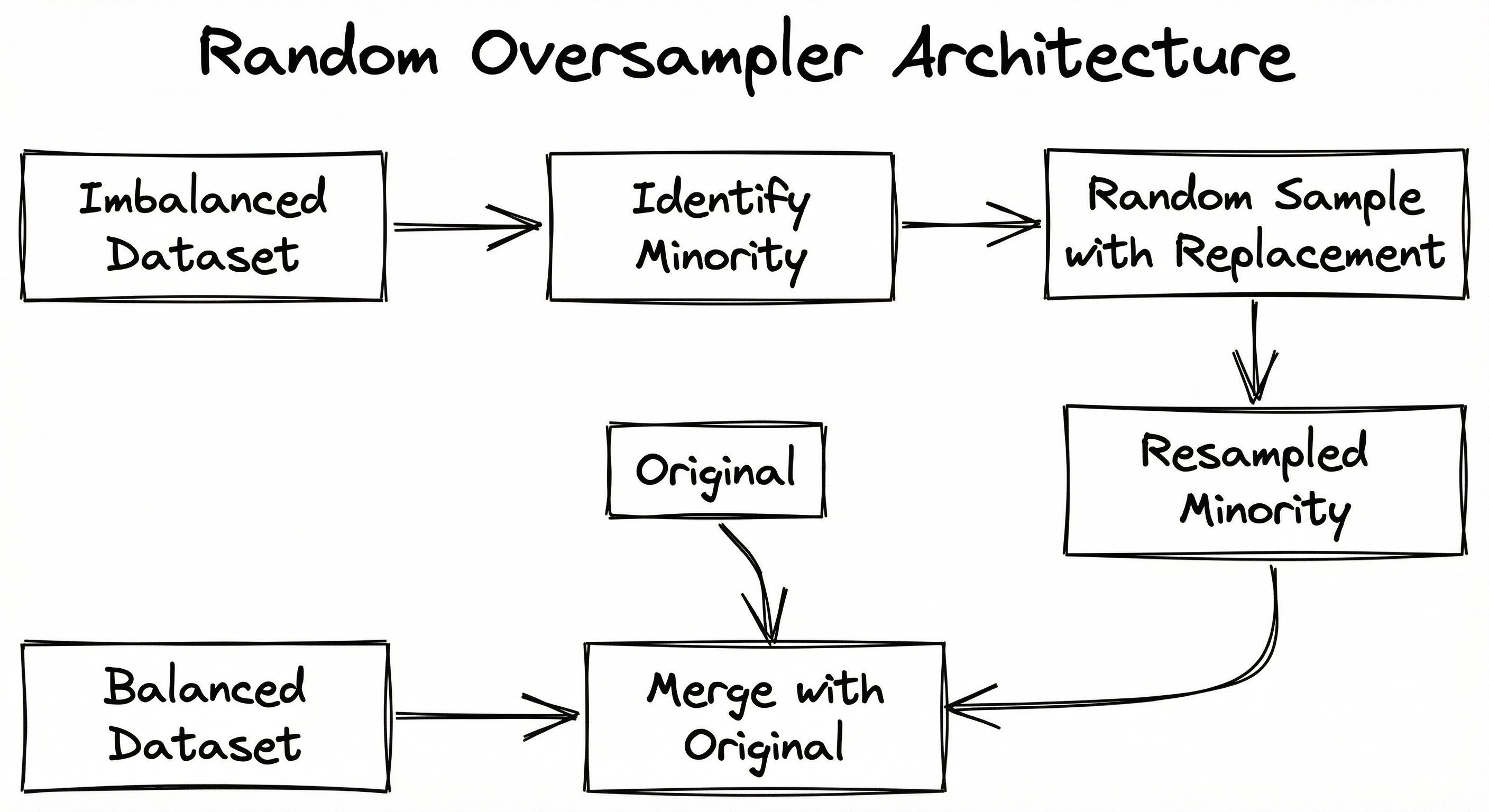
The branching at the shrinkage decision point is the key architectural distinction between naive random oversampling and the ROSE smoothed bootstrap variant. When shrinkage is None, the system is a simple bootstrap sampler. When shrinkage is provided, the system estimates the class-conditional covariance matrix and adds scaled Gaussian noise to each drawn sample.
Key Components
Class Distribution Analyzer
Counts samples per class, identifies minority and majority classes, and computes the number of new samples needed based on the sampling_strategy parameter. For multi-class problems, applies the strategy to each underrepresented class independently.
Bootstrap Sampler
Draws minority class samples uniformly at random with replacement. This is the core engine for naive random oversampling. Uses the random state for reproducibility.
Covariance Estimator (Smoothed Mode)
Computes the sample covariance matrix for each minority class when the shrinkage parameter is set. This matrix captures the spread and correlations of minority class features, which is used to generate realistic perturbations.
Perturbation Generator (Smoothed Mode)
For each drawn sample, generates a random perturbation vector from and adds it to the original sample. The shrinkage factor controls how far synthetic samples can deviate from originals.
Dataset Assembler
Merges original samples (all classes untouched) with the newly generated minority samples. Assigns correct class labels to new samples and returns the combined, balanced dataset.
Data Flow
Input Flow: The algorithm receives an imbalanced dataset and the target sampling_strategy. It separates samples by class and identifies which classes need augmentation.
Processing Flow (Naive Mode): For each underrepresented class, the bootstrap sampler draws the required number of samples with replacement from the existing minority pool. Each drawn sample is an exact copy of an original sample. No feature transformations are applied.
Processing Flow (Smoothed Mode): The covariance estimator first computes for each minority class. Then, for each drawn sample, the perturbation generator adds scaled Gaussian noise. The noise magnitude is proportional to the shrinkage parameter and the class covariance, ensuring perturbations respect the natural spread of the data.
Output Flow: New samples are labeled with their respective minority class labels and combined with the original dataset. The output preserves all original samples unchanged -- only the minority classes gain additional (possibly perturbed) copies.
A flow from 'Imbalanced Dataset' through class distribution analysis, a conditional branch on whether shrinkage is enabled (leading to either simple bootstrap sampling or covariance-based smoothed sampling), and finally combining with original data to produce a 'Balanced Dataset'.
How to Implement
Implementation Approaches
Random oversampling is primarily used through the imbalanced-learn (imblearn) library, which provides RandomOverSampler as a scikit-learn-compatible transformer. The API is identical to SMOTE -- fit_resample(X, y) -- making it trivial to swap between techniques in an experiment pipeline.
Key configuration decisions:
- Naive vs. smoothed: Set
shrinkage=Nonefor exact duplication orshrinkage=<float>for ROSE-style smoothed bootstrap - Sampling strategy: Usually
'auto'(balance to 50-50) or a float for partial oversampling - With replacement: Always true for standard random oversampling (this is the default and cannot be changed)
For production systems, random oversampling is applied as a preprocessing step in the training pipeline only. The oversampled data is used for training; validation and test sets remain untouched with their original class distribution.
Cost Note: Random oversampling is essentially free computationally. Even on a modest 2-core machine (~0.17/hr, ~₹14/hr), smoothed oversampling of 1M samples completes in under 10 seconds.
from imblearn.over_sampling import RandomOverSampler
from sklearn.datasets import make_classification
from sklearn.model_selection import train_test_split
from sklearn.ensemble import GradientBoostingClassifier
from sklearn.metrics import classification_report
import numpy as np

# Create imbalanced dataset (1:99 ratio)
X, y = make_classification(
    n_classes=2,
    weights=[0.01, 0.99],
    n_samples=10000,
    n_features=20,
    n_informative=10,
    random_state=42
)

print(f"Original distribution: {np.bincount(y)}")
# Output: [100, 9900]

# Split FIRST, then oversample training data only
X_train, X_test, y_train, y_test = train_test_split(
    X, y, test_size=0.2, random_state=42, stratify=y
)

print(f"Train distribution (before): {np.bincount(y_train)}")
# Output: [80, 7920]

# Apply naive random oversampling (exact duplication)
ros = RandomOverSampler(sampling_strategy='auto', random_state=42)
X_train_ros, y_train_ros = ros.fit_resample(X_train, y_train)

print(f"Train distribution (after):  {np.bincount(y_train_ros)}")
# Output: [7920, 7920] — perfectly balanced

# Train on oversampled data, evaluate on original test set
clf = GradientBoostingClassifier(n_estimators=100, random_state=42)
clf.fit(X_train_ros, y_train_ros)

y_pred = clf.predict(X_test)
print(classification_report(y_test, y_pred))
This is the standard random oversampling workflow. Three critical details: (1) We split before oversampling -- oversampling the full dataset and then splitting would leak duplicate samples into the test set; (2) sampling_strategy='auto' balances to 50-50; (3) Evaluation uses the original imbalanced test distribution, which reflects real-world conditions.
from imblearn.over_sampling import RandomOverSampler
from sklearn.datasets import make_classification
import numpy as np

# Create imbalanced dataset
X, y = make_classification(
    n_classes=2,
    weights=[0.05, 0.95],
    n_samples=5000,
    n_features=10,
    n_informative=6,
    random_state=42
)

print(f"Original: {np.bincount(y)}")
# Output: [250, 4750]

# Naive oversampling (exact duplicates)
ros_naive = RandomOverSampler(shrinkage=None, random_state=42)
X_naive, y_naive = ros_naive.fit_resample(X, y)

# Smoothed bootstrap with default shrinkage
n_min = np.sum(y == 0)  # minority count
d = X.shape[1]           # feature dimensionality
shrinkage_optimal = n_min ** (-1 / (d + 4))  # Silverman rule
print(f"Optimal shrinkage (Silverman): {shrinkage_optimal:.4f}")

ros_smoothed = RandomOverSampler(shrinkage=shrinkage_optimal, random_state=42)
X_smoothed, y_smoothed = ros_smoothed.fit_resample(X, y)

# Verify: smoothed samples are NOT exact duplicates
original_minority = X[y == 0]
new_samples_smoothed = X_smoothed[len(X):]

# Check if any new sample exactly matches an original
exact_matches = 0
for sample in new_samples_smoothed:
    if any(np.allclose(sample, orig) for orig in original_minority):
        exact_matches += 1

print(f"Exact matches in smoothed mode: {exact_matches}/{len(new_samples_smoothed)}")
# Output: 0 — no exact duplicates with shrinkage > 0

# Higher shrinkage = more dispersion
ros_high = RandomOverSampler(shrinkage=2.0, random_state=42)
X_high, y_high = ros_high.fit_resample(X, y)

print(f"Std of new samples (naive):    {np.std(X_naive[len(X):], axis=0).mean():.4f}")
print(f"Std of new samples (smoothed): {np.std(X_smoothed[len(X):], axis=0).mean():.4f}")
print(f"Std of new samples (high s):   {np.std(X_high[len(X):], axis=0).mean():.4f}")
This demonstrates the difference between naive and smoothed oversampling. The shrinkage parameter controls how much Gaussian noise is added to duplicated samples. With shrinkage=None, you get exact copies. With shrinkage > 0, every new sample is a unique perturbation of an original. The Silverman rule provides an asymptotically optimal shrinkage value under normality assumptions. Higher shrinkage disperses new samples further from originals -- useful for reducing overfitting but risky if set too high (samples may drift into majority class territory).
from imblearn.pipeline import Pipeline as ImbPipeline
from imblearn.over_sampling import RandomOverSampler
from sklearn.preprocessing import StandardScaler
from sklearn.linear_model import LogisticRegression
from sklearn.model_selection import cross_val_score, StratifiedKFold
from sklearn.datasets import make_classification
import numpy as np

# Create imbalanced dataset
X, y = make_classification(
    n_classes=2,
    weights=[0.02, 0.98],
    n_samples=10000,
    n_features=15,
    n_informative=8,
    random_state=42
)

# Build pipeline with oversampling
# Note: use imblearn.pipeline.Pipeline, NOT sklearn.pipeline.Pipeline
pipeline = ImbPipeline([
    ('scaler', StandardScaler()),
    ('oversampler', RandomOverSampler(
        sampling_strategy=0.5,  # Target 50% minority-to-majority ratio
        shrinkage=0.3,          # Mild smoothing
        random_state=42
    )),
    ('classifier', LogisticRegression(
        C=1.0,
        class_weight=None,  # Don't use class_weight AND oversampling together
        max_iter=1000,
        random_state=42
    )),
])

# Cross-validation with stratified folds
cv = StratifiedKFold(n_splits=5, shuffle=True, random_state=42)
scores = cross_val_score(
    pipeline, X, y,
    cv=cv,
    scoring='f1',  # F1 is more informative than accuracy for imbalanced data
    n_jobs=-1
)

print(f"F1 scores per fold: {scores}")
print(f"Mean F1: {scores.mean():.4f} (+/- {scores.std():.4f})")
The imblearn.pipeline.Pipeline (not sklearn.pipeline.Pipeline) correctly applies oversampling only to the training fold in cross-validation. This prevents data leakage: each fold's test set remains untouched. Two important choices here: (1) sampling_strategy=0.5 targets a 1:2 minority-to-majority ratio instead of full balance -- partial oversampling often performs better than full balance; (2) We use class_weight=None in the classifier because we're already addressing imbalance via oversampling -- combining both can overcorrect.
from imblearn.over_sampling import RandomOverSampler, SMOTE
from sklearn.datasets import make_classification
from sklearn.model_selection import RepeatedStratifiedKFold, cross_validate
from sklearn.ensemble import RandomForestClassifier
import numpy as np
from imblearn.pipeline import Pipeline as ImbPipeline

# Create a moderately imbalanced dataset
X, y = make_classification(
    n_classes=2,
    weights=[0.05, 0.95],
    n_samples=5000,
    n_features=20,
    n_informative=12,
    n_clusters_per_class=3,
    random_state=42
)

# Define three oversampling strategies
strategies = {
    'No Resampling': None,
    'Naive ROS': RandomOverSampler(shrinkage=None, random_state=42),
    'Smoothed ROS (s=0.5)': RandomOverSampler(shrinkage=0.5, random_state=42),
    'SMOTE (k=5)': SMOTE(k_neighbors=5, random_state=42),
}

cv = RepeatedStratifiedKFold(n_splits=5, n_repeats=3, random_state=42)
clf = RandomForestClassifier(n_estimators=100, random_state=42)

for name, sampler in strategies.items():
    if sampler is None:
        pipeline = clf
    else:
        pipeline = ImbPipeline([
            ('sampler', sampler),
            ('clf', clf),
        ])

    results = cross_validate(
        pipeline, X, y,
        cv=cv,
        scoring=['f1', 'roc_auc', 'average_precision'],
        n_jobs=-1
    )

    print(f"{name:25s} | F1: {results['test_f1'].mean():.3f} "
          f"| AUC: {results['test_roc_auc'].mean():.3f} "
          f"| AP: {results['test_average_precision'].mean():.3f}")
This head-to-head comparison reveals the relative performance of the three approaches across multiple metrics. In many real-world scenarios, you'll find that naive ROS and SMOTE perform similarly on tree-based models (which are naturally robust to duplicates), while the smoothed bootstrap variant may edge ahead when combined with linear models or on smaller datasets. The RepeatedStratifiedKFold with 3 repeats gives more stable estimates than a single 5-fold split.
# imbalanced-learn RandomOverSampler configuration
# Naive mode (exact duplication)
RandomOverSampler:
  sampling_strategy: 'auto'    # Balance to 50-50
  random_state: 42
  shrinkage: null               # No perturbation

# Smoothed bootstrap (ROSE) mode
RandomOverSampler:
  sampling_strategy: 0.5        # Target 50% minority/majority ratio
  random_state: 42
  shrinkage: 0.3                # Mild Gaussian perturbation

# Per-class shrinkage (advanced)
RandomOverSampler:
  sampling_strategy: 'auto'
  random_state: 42
  shrinkage:
    0: 0.5                      # Shrinkage for class 0
    1: 0.2                      # Shrinkage for class 1
Common Implementation Mistakes
- ●
Oversampling before train-test split: This is the most dangerous mistake. If you oversample the full dataset, duplicate samples will appear in both training and test sets, creating data leakage. Your test metrics will look artificially inflated. Always split first, then oversample only the training fold.
- ●
Combining random oversampling with class weights: Both techniques serve the same purpose -- amplifying the minority class signal. Using both together double-compensates, often causing the model to over-predict the minority class (low precision, high false positive rate). Choose one or the other, not both.
- ●
Oversampling minority to exact 50-50 balance: Full balance isn't always optimal. For highly imbalanced data (IR > 50), partial oversampling (e.g.,
sampling_strategy=0.3) often yields better calibrated probabilities and better F1 scores. Experiment with the target ratio. - ●
Using naive oversampling with memorization-prone models: Exact duplication is most harmful with models that can memorize training examples -- k-NN, decision stumps, small neural networks. Tree ensembles (Random Forest, XGBoost) are naturally more robust because individual trees see different bootstrap samples. Always consider model choice when deciding between naive and smoothed oversampling.
- ●
Setting shrinkage too high: Excessive perturbation pushes synthetic samples into majority class territory, creating noisy labels. Start with the Silverman optimal () and only increase if overfitting persists. A shrinkage value > 2.0 is almost always too high.
- ●
Ignoring the effect on probability calibration: Oversampling changes the prior probability of each class in the training data. Model-predicted probabilities will no longer reflect the true class distribution. If you need calibrated probabilities (for ranking or decision-making), apply post-hoc calibration (Platt scaling or isotonic regression) after training.
When Should You Use This?
Use When
Your dataset has mixed feature types (categorical + numerical + text embeddings) where SMOTE's distance-based interpolation doesn't make sense -- random oversampling works regardless of feature type
Computational budget is tight and you need the fastest possible resampling: random oversampling is O(n), SMOTE is O(n^2) for the k-NN search
You're using regularized tree ensembles (Random Forest, XGBoost, LightGBM) that naturally resist overfitting from duplicated samples
The minority class has very few samples (< 50) where k-NN in SMOTE becomes unreliable due to sparse neighborhoods
You need a quick baseline for comparison before investing in more sophisticated resampling techniques
Your pipeline requires sparse matrix support -- smoothed bootstrap mode is not available for sparse matrices, but naive random oversampling works fine
You want reproducible, auditable results: naive ROS produces only real data points (duplicates), not synthetic interpolations that may not represent valid data
Avoid When
Your model is highly susceptible to overfitting on duplicated examples (e.g., k-NN classifiers, single decision trees) AND you cannot use the smoothed bootstrap variant
The minority class samples contain significant label noise -- duplicating noisy samples amplifies the noise, making the problem worse
You need synthetic samples that explore the feature space beyond existing examples -- SMOTE or ADASYN generate points in between existing samples, providing better boundary coverage
The imbalance ratio is extreme (> 100:1) AND you have enough minority samples (> 500) for SMOTE to work well -- SMOTE's interpolation provides more diversity than duplication at these ratios
You're working with high-dimensional continuous features where the smoothed bootstrap covariance matrix becomes ill-conditioned (d >> n_min)
Your evaluation metric is primarily recall-oriented and boundary coverage matters more than class balance -- SMOTE variants like Borderline-SMOTE specifically target the decision boundary
Key Tradeoffs
The Fundamental Tradeoff: Simplicity vs. Diversity
Naive random oversampling creates zero new information. Every "new" sample is an exact copy of an existing one. SMOTE, by contrast, creates genuinely new points in feature space via interpolation. The tradeoff is clear: random oversampling is safer (no risk of generating invalid samples) but less diverse (no new patterns).
For well-regularized models (Random Forest, gradient boosting), this tradeoff often doesn't matter -- the model's own regularization prevents overfitting on duplicates. For models with high capacity and low regularization (deep nets with small datasets, k-NN), the lack of diversity from naive oversampling can be a real problem.
Smoothed Bootstrap: The Middle Ground
The shrinkage parameter offers a smooth interpolation between naive duplication (shrinkage=0) and ROSE-style smoothed bootstrap (shrinkage>0). This gives you a dial:
| Shrinkage | Behavior | Best For |
|---|---|---|
| 0 (None) | Exact duplication | Tree ensembles, sparse data |
| 0.1-0.5 | Mild perturbation | Linear models, moderate regularization |
| 0.5-1.0 | Moderate perturbation | Neural networks, well-behaved features |
| > 1.0 | Heavy perturbation | Rarely recommended -- samples may cross class boundaries |
When Random Oversampling Beats SMOTE
This is counterintuitive, but random oversampling outperforms SMOTE in several scenarios:
- Very small minority class (< 30 samples): SMOTE's k-NN becomes unreliable
- High-dimensional sparse features: Interpolation in sparse spaces creates dense vectors that don't represent real data
- Categorical or mixed features: SMOTE requires meaningful distance metrics; standard Euclidean distance doesn't work for one-hot encoded categoricals
- Extreme noise: SMOTE can amplify noise by interpolating between a clean sample and a noisy/mislabeled one
Rule of Thumb: Start with random oversampling as your baseline. If it underperforms SMOTE by more than 2-3% F1 on your validation set, investigate whether the diversity from SMOTE is genuinely helping or just fitting noise.
Alternatives & Comparisons
SMOTE generates synthetic samples by interpolating between k-nearest minority neighbors, providing more diversity than random oversampling. Choose SMOTE when you have sufficient minority samples (> 50), continuous features with meaningful distances, and a model that benefits from boundary-region coverage. Choose random oversampling for mixed/categorical features, very small minority classes, or when you need a simpler, faster baseline.
ADASYN (Adaptive Synthetic Sampling) adaptively generates more synthetic samples for minority instances that are harder to classify (near the decision boundary). It provides better boundary coverage than random oversampling but is more expensive and can amplify noise in borderline regions. Use ADASYN when boundary precision matters; use random oversampling for general-purpose balancing.
Random undersampling removes majority class samples instead of duplicating minority ones. It avoids the overfitting risk of oversampling but discards potentially valuable majority class information. Prefer undersampling when the dataset is large (> 100K samples) and you can afford to lose majority class data. Prefer oversampling when every sample is precious.
Borderline-SMOTE focuses synthetic generation exclusively on minority samples near the decision boundary, ignoring safe interior points. This provides more targeted boundary coverage than random oversampling's uniform duplication. Choose Borderline-SMOTE when the decision boundary is the bottleneck; choose random oversampling when the entire minority class needs amplification.
SMOTE+ENN combines oversampling with Edited Nearest Neighbors cleaning, removing noisy samples after generation. This addresses the noise amplification problem that affects both random oversampling and vanilla SMOTE. Use SMOTE+ENN when label noise is a concern; use random oversampling when data quality is high and you want simplicity.
Pros, Cons & Tradeoffs
Advantages
Zero hyperparameters in naive mode -- no k-neighbors, no distance metrics, nothing to tune. Set
sampling_strategyand go. This makes it the fastest technique to prototype and the hardest to misconfigure.Universal feature type support: works with continuous, categorical, sparse, binary, and mixed features without modification. SMOTE requires meaningful distance metrics, which limits it to continuous features (or SMOTE-NC for mixed data).
Computationally trivial: time complexity vs SMOTE's k-NN search. For a dataset with 1M minority samples, random oversampling takes <1 second vs SMOTE's potential minutes on comparable hardware.
Smoothed bootstrap via shrinkage provides a middle ground between naive duplication and full synthetic generation, reducing overfitting while maintaining simplicity. The ROSE integration makes random oversampling surprisingly flexible.
Equivalent to class weighting for SGD-trained models -- enables direct comparison between data-level and algorithm-level imbalance handling, which is valuable for ablation studies and production debugging.
No risk of generating invalid samples: duplicated samples are by definition valid members of the minority class. SMOTE can generate synthetic samples in regions between classes that don't represent real data, especially in high-dimensional spaces.
Preserves data interpretability: every sample in the oversampled dataset is a real observed data point (or small perturbation thereof), which matters in regulated domains (healthcare, finance) where model auditors need to trace predictions back to real observations.
Disadvantages
Overfitting risk with exact duplication: the model sees identical copies of the same samples, which can lead to memorization rather than generalization. This is most severe with high-capacity models (deep nets, k-NN) and small minority classes.
No new information created: unlike SMOTE's interpolation, naive random oversampling does not expand the feature space coverage of the minority class. The decision boundary learned from 100 unique minority samples is identical whether you see them 1x or 100x each (for models with perfect memory).
Increases training set size, which can slow training for expensive models (neural networks, SVMs with RBF kernels). Oversampling a 1:100 dataset to 50-50 nearly doubles the training set size.
Probability calibration distortion: oversampling changes the effective prior probability of each class. Model-predicted probabilities no longer reflect the true class distribution without post-hoc recalibration.
Amplifies label noise: if some minority class samples are mislabeled, duplication amplifies those errors. A mislabeled sample duplicated 50 times has 50x the influence on the model.
Smoothed bootstrap limitations: the covariance-based perturbation in ROSE mode doesn't work with sparse matrices and assumes approximately Gaussian feature distributions. For highly non-Gaussian data (multi-modal, heavy-tailed), the perturbation can produce unrealistic samples.
Diminishing returns at extreme ratios: when the imbalance ratio exceeds 1000:1, random oversampling requires creating 1000 copies of each minority sample. At this level, even well-regularized models struggle with the extreme duplication.
Failure Modes & Debugging
Severe overfitting from naive duplication
Cause
Exact copies of minority samples are repeated dozens or hundreds of times, causing the model to memorize specific instances rather than learning generalizable patterns. Most severe with high-capacity models (k-NN, deep networks) on small minority classes (< 50 samples).
Symptoms
Training F1 or AUC is near-perfect (> 0.99) while validation/test F1 drops significantly (gap > 0.15). The model performs well on samples it has seen but poorly on new minority examples. Learning curves show increasing gap between training and validation loss.
Mitigation
Switch to smoothed bootstrap mode by setting shrinkage to the Silverman optimal value (). Alternatively, use a regularized model (Random Forest, gradient boosting with max_depth limits, or L2-regularized logistic regression). For extreme cases, consider SMOTE or ADASYN instead.
Data leakage from pre-split oversampling
Cause
Oversampling is applied to the full dataset before train-test split. Duplicated minority samples appear in both training and test sets, meaning the model is tested on data it has literally trained on.
Symptoms
Test metrics are unrealistically high (e.g., F1 > 0.95 on a task where domain experts expect 0.70-0.80). Performance collapses in production when the model sees genuinely new data. A/B tests show the model performs far worse than offline metrics suggested.
Mitigation
Always split first, then oversample. Use imblearn.pipeline.Pipeline for cross-validation to ensure oversampling is applied only within each training fold. Add a validation check that compares sample counts before and after the split to catch accidental leakage.
Noise amplification from mislabeled minority samples
Cause
Some minority samples have incorrect labels (a legitimate transaction labeled as fraud, a benign tumor labeled as malignant). Random oversampling duplicates these mislabeled samples, amplifying their harmful influence on the decision boundary.
Symptoms
The model predicts the minority class in unexpected regions of feature space. Precision for the minority class is unexpectedly low while recall is moderate. Feature importance analysis shows the model relying on features that domain experts consider irrelevant.
Mitigation
Apply data cleaning before oversampling: use Edited Nearest Neighbors (ENN) or Tomek Links to remove potentially mislabeled samples. Alternatively, use SMOTE+ENN which combines oversampling with post-hoc noise cleaning. For high-stakes applications, conduct a label audit of the minority class before any resampling.
Probability calibration collapse
Cause
Oversampling changes the effective class prior from (e.g.) 1:99 to 50:50. The model's predicted probabilities now reflect the artificial 50:50 distribution rather than the true 1:99 distribution. A predicted probability of 0.5 might actually correspond to a true probability of 0.01.
Symptoms
Predicted probabilities are dramatically overestimated for the minority class. A calibration plot (reliability diagram) shows severe miscalibration. Threshold-based decision making produces unexpected false positive rates.
Mitigation
Apply post-hoc calibration after training: Platt scaling (logistic regression on predicted probabilities) or isotonic regression using a held-out calibration set with the original class distribution. Alternatively, use partial oversampling (sampling_strategy < 1.0) to reduce the distribution shift.
Smoothed bootstrap generating out-of-class samples
Cause
The shrinkage parameter is set too high, causing Gaussian perturbations large enough to push synthetic samples into majority class territory. This is especially problematic when minority and majority classes are close in feature space or when the minority class has high variance.
Symptoms
Model performance decreases when using smoothed oversampling compared to naive duplication. The minority class precision drops while recall may increase. Visualization of synthetic samples (in 2D PCA/t-SNE space) shows new samples overlapping with majority class clusters.
Mitigation
Start with the Silverman-optimal shrinkage () and tune downward. Visualize synthetic samples in reduced dimensions to verify they remain within minority class regions. For datasets where classes overlap significantly, prefer naive duplication (shrinkage=None) or consider cost-sensitive learning instead.
Training time explosion from extreme oversampling
Cause
When the imbalance ratio is extreme (e.g., 1:1000), oversampling to 50-50 balance increases the training set by nearly 2x. For models with super-linear training cost (SVMs: , neural nets: ), this can make training prohibitively slow or expensive.
Symptoms
Training time increases from minutes to hours. GPU memory exhaustion for neural network training. Cloud compute costs spike unexpectedly. Batch gradient descent becomes impractical.
Mitigation
Use partial oversampling (sampling_strategy=0.3 or 0.5) instead of full balance. For neural networks, prefer class-weighted loss functions over data-level oversampling. For SVMs, consider random undersampling of the majority class instead. Budget training time before committing to a full oversampling strategy.
Placement in an ML System
Where Does It Sit in the Pipeline?
Random oversampling occupies a very specific position in the ML pipeline: after the train-test split and before model training. This placement is non-negotiable -- oversampling before splitting creates data leakage, and oversampling during inference makes no sense (you only resample training data).
In a typical production pipeline at a company like Razorpay or Paytm building a fraud detection model:
- Data ingestion pulls transaction logs from the data warehouse
- Feature engineering computes features (transaction amount, velocity, device fingerprint)
- Train-test split creates stratified partitions preserving the original class ratio
- Random oversampling balances the training partition
- Model training fits on the balanced data
- Model evaluation measures on the original imbalanced test set
Random oversampling is strictly a training-time operation. It does not appear in the inference pipeline. The trained model receives raw, unmodified inputs at serving time.
Key Insight: Unlike feature engineering transforms (scaling, encoding) that must be applied at both training and inference time, random oversampling has no inference-time component. This simplifies the serving pipeline but means the model must generalize from oversampled training data to the original imbalanced distribution.
Pipeline Stage
Data Preprocessing / Training
Upstream
- Data validation
- Feature engineering
- Train-test split
Downstream
- Model training
- Hyperparameter tuning
- Model evaluation
Scaling Bottlenecks
Random oversampling itself is not the bottleneck -- it's for naive mode and for covariance estimation in smoothed mode. The bottleneck is the downstream effect: oversampling increases the training set size, which directly impacts training time for the model.
For a dataset with 1M majority and 10K minority samples, oversampling to 50-50 creates ~990K new samples, nearly doubling the training set. For XGBoost, this might add 30-60 seconds of training time. For a neural network with 100 epochs, it could add hours.
The memory footprint scales linearly: bytes for float32 features. Oversampling 10K samples with 1000 features to 1M total requires ~4GB additional memory.
At truly large scale (> 10M total samples after oversampling), consider:
- Partial oversampling (
sampling_strategy < 1.0) to limit growth - Online/streaming learning with weighted sampling instead of materializing duplicates
- Distributed training frameworks that handle the larger dataset across nodes
Production Case Studies
In a study using the American Express credit card fraud detection dataset, researchers compared random oversampling (ROS), random undersampling (RUS), and SMOTE for handling severe class imbalance (< 1% fraud rate). ROS combined with XGBoost achieved 0.99 precision and 0.99 accuracy, performing comparably to SMOTE-based approaches while requiring significantly less preprocessing time. The study demonstrated that for tree-based ensemble models, the simplicity advantage of ROS over SMOTE is meaningful.
Random oversampling matched SMOTE performance (within 1% F1) when paired with XGBoost, while reducing preprocessing time by approximately 60% on the 140K-transaction dataset.
A 2025 study on stroke prediction compared random oversampling, SMOTE, ADASYN, and SMOTE-Tomek for handling imbalanced clinical data. The dataset contained standard clinical features (age, BMI, glucose levels, hypertension history). Random oversampling combined with SVM (RBF kernel) achieved the best overall results among all resampling-model combinations tested, with sensitivity of 89.87%, specificity of 94.91%, and G-mean of 92.36%.
ROS-SVM outperformed SMOTE-based approaches by 2-4% on G-mean, demonstrating that simple oversampling can be optimal when paired with the right classifier, even for medical diagnosis tasks.
Researchers applied random oversampling and SMOTE to early cervical cancer detection using Indonesian patient data. The dataset exhibited extreme imbalance (< 5% positive cases), a common challenge in cancer screening datasets in developing nations where positive cases are rare. The study compared both techniques with Naive Bayes classifiers and found that ROS achieved comparable accuracy to SMOTE while being more interpretable for the clinical team.
Random oversampling enabled the Naive Bayes classifier to achieve improved recall for cancer-positive cases, making the screening tool more suitable for deployment in resource-constrained Indonesian healthcare settings.
A fintech e-commerce platform deployed a fraud detection system processing approximately 140,000 transactions (October 2021 to April 2024). The system used oversampling techniques including random oversampling as part of a multi-strategy approach to handle severe class imbalance. The production system included a real-time fraud scoring API with ongoing model monitoring to track data drift and evolving fraud patterns.
After six months in production, the platform achieved a 40% reduction in undetected fraud cases and associated financial losses. The system included scheduled retraining using newly collected data with automated resampling adjustments.
Tooling & Ecosystem
The canonical Python library for resampling. RandomOverSampler supports naive duplication and smoothed bootstrap (ROSE) via the shrinkage parameter. Fully compatible with scikit-learn pipelines via imblearn.pipeline.Pipeline. The most widely used implementation in both research and production.
The original R implementation of Random Over-Sampling Examples by Menardi, Lunardon, and Torelli. Implements smoothed bootstrap with kernel density estimation. Includes ROSE.eval for evaluating accuracy of models trained on ROSE-generated data. The theoretical foundation for imbalanced-learn's shrinkage feature.
While not a resampling tool, scikit-learn's class_weight='balanced' parameter achieves mathematically equivalent results to random oversampling for SGD-trained models. Available in LogisticRegression, SVC, RandomForestClassifier, and most other sklearn estimators. The algorithm-level alternative to data-level oversampling.
Extends imbalanced-learn with ensemble methods that integrate resampling into the ensemble training loop. Provides RandomOverSampler as a component within bagging and boosting frameworks designed for imbalanced data. Useful when you want per-base-learner resampling rather than one-time dataset resampling.
Apache Spark provides class weighting for distributed training but does not have a built-in random oversampler. For Spark-based pipelines, you can implement random oversampling using DataFrame operations (sample with replacement). Essential for large-scale datasets that don't fit in memory on a single node.
TensorFlow's tf.data.Dataset API supports oversampling via .repeat() on minority class datasets combined with .sample_from_datasets() for online class-balanced sampling. This avoids materializing the oversampled dataset in memory -- critical for large-scale deep learning pipelines. Equivalent to random oversampling applied per-batch rather than pre-training.
Research & References
Chawla, N.V., Bowyer, K.W., Hall, L.O., Kegelmeyer, W.P. (2002)Journal of Artificial Intelligence Research, Vol. 16, pp. 321-357
The landmark paper that introduced SMOTE and used random oversampling as the primary baseline. Demonstrated that SMOTE outperforms naive random oversampling on several benchmarks, establishing the comparison framework that has shaped imbalanced learning research for two decades.
Menardi, G., Torelli, N. (2014)Data Mining and Knowledge Discovery, Vol. 28, pp. 92-122
Introduced the ROSE (Random Over-Sampling Examples) method -- smoothed bootstrap oversampling with kernel density estimation. This paper provides the theoretical foundation for the shrinkage parameter in imbalanced-learn's RandomOverSampler.
He, H., Garcia, E.A. (2009)IEEE Transactions on Knowledge and Data Engineering, Vol. 21, No. 9, pp. 1263-1284
Comprehensive survey of imbalanced learning that catalogs random oversampling as a foundational data-level technique. Discusses overfitting risks, compares with undersampling and cost-sensitive approaches, and establishes the taxonomy used by subsequent research.
Branco, P., Torgo, L., Ribeiro, R.P. (2016)ACM Computing Surveys, Vol. 49, No. 2
Extensive survey covering both classification and regression under imbalance. Positions random oversampling within a broader taxonomy of data-level, algorithm-level, and ensemble approaches. Discusses the theoretical equivalence between oversampling and cost-sensitive learning.
van den Goorbergh, R., van Smeden, M., Timmerman, D., Zwinderman, A.H. (2022)Journal of Big Data
Empirical study finding that random oversampling generally does not improve internal/external validation performance in large observational health databases. A cautionary result that highlights the importance of evaluating resampling techniques on your specific dataset rather than assuming universal benefit.
Obaid, O.I., et al. (2024)Frontiers in Digital Health
2024 comprehensive review of oversampling techniques for medical multi-class imbalance. Evaluates random oversampling alongside SMOTE, ADASYN, and generative approaches. Finds that random oversampling remains competitive for certain medical classification tasks, particularly with ensemble classifiers.
Interview & Evaluation Perspective
Common Interview Questions
- ●
What is the difference between random oversampling and SMOTE? When would you prefer one over the other?
- ●
What is the main risk of random oversampling and how would you mitigate it?
- ●
Explain why random oversampling is mathematically equivalent to class weighting for SGD-trained models.
- ●
You have a fraud detection dataset with 0.1% positive rate and mixed categorical/numerical features. How would you handle the imbalance?
- ●
What is the shrinkage parameter in imbalanced-learn's RandomOverSampler? When would you use it?
- ●
Why should you never apply oversampling before the train-test split?
Key Points to Mention
- ●
Random oversampling is the simplest resampling technique and serves as the universal baseline for imbalanced learning. Every sophistication (SMOTE, ADASYN, Borderline-SMOTE) is measured against it.
- ●
The primary risk is overfitting from exact duplication, but this is model-dependent: tree ensembles are naturally robust to duplicates due to bootstrap sampling within each tree, while k-NN and linear models are more susceptible.
- ●
The smoothed bootstrap (ROSE) variant via the shrinkage parameter adds Gaussian perturbation to duplicated samples, reducing overfitting risk while maintaining the simplicity of the random oversampling framework.
- ●
Random oversampling works with ANY feature type (categorical, continuous, sparse, mixed), while SMOTE requires continuous features with meaningful distance metrics.
- ●
Always oversample AFTER the train-test split -- never before. Use
imblearn.pipeline.Pipelinefor correct cross-validation behavior. - ●
For production systems, consider whether class weighting (
class_weight='balanced') achieves the same result without modifying the dataset. For SGD-trained models, the two approaches are mathematically equivalent.
Pitfalls to Avoid
- ●
Claiming that random oversampling always leads to overfitting -- this is model-dependent. Tree ensembles are naturally resistant due to their own bootstrap sampling.
- ●
Dismissing random oversampling as 'too simple' without acknowledging that it outperforms SMOTE on mixed feature types, very small minority classes, and noisy datasets.
- ●
Forgetting the smoothed bootstrap (ROSE/shrinkage) variant, which significantly addresses the overfitting concern while keeping the simplicity advantage.
- ●
Not mentioning the equivalence with class weighting -- this shows deeper understanding of why oversampling works at the optimization level.
Senior-Level Expectation
A senior candidate should discuss random oversampling within the broader context of imbalanced learning strategies: data-level (oversampling, undersampling, combined), algorithm-level (class weights, cost-sensitive learning, threshold adjustment), and ensemble-level (BalancedBagging, EasyEnsemble). They should articulate when random oversampling is the right choice (mixed features, small minority class, regulatory requirements for real data) and when to move to alternatives. They should know the smoothed bootstrap (ROSE) extension and its connection to kernel density estimation. At the system level, they should discuss how oversampling interacts with other pipeline components: cross-validation leakage, probability calibration, feature scaling order, and the fact that oversampling is a training-time-only operation with no inference footprint. For Indian tech context, discussing how fraud detection at scale (Razorpay, Paytm, PhonePe) handles class imbalance in production -- typically class weighting for online models and oversampling for batch-trained models -- demonstrates real-world awareness.
Summary
Random oversampling is the simplest and most universal technique for addressing class imbalance in machine learning. At its core, it duplicates minority class samples with replacement until the desired class balance is achieved. Despite its simplicity, it remains a production workhorse -- competitive with SMOTE on many real-world benchmarks, particularly when paired with regularized tree ensembles.
The technique's evolution is worth noting. The modern implementation in imbalanced-learn extends naive duplication with the shrinkage parameter (inspired by the ROSE method of Menardi and Torelli, 2014), enabling smoothed bootstrap sampling that adds controlled Gaussian perturbation to duplicated samples. This single parameter transforms random oversampling from a blunt instrument prone to overfitting into a nuanced tool with a smooth tradeoff between duplication fidelity and sample diversity.
The key decisions for practitioners are: (1) naive vs. smoothed -- use shrinkage > 0 when working with models susceptible to memorization (neural networks, k-NN) and shrinkage=None for tree ensembles; (2) oversampling vs. class weighting -- they're mathematically equivalent for SGD-trained models, so prefer class weighting when the dataset size increase from oversampling would be costly; and (3) random oversampling vs. SMOTE -- prefer random oversampling for mixed/categorical features, very small minority classes, and sparse data where SMOTE's interpolation produces invalid samples.
Random oversampling endures because it embodies a fundamental principle of engineering: the simplest solution that works is often the best solution. It's the technique you start with, the baseline you measure against, and -- more often than you'd expect -- the technique you ship to production.