NearMiss in Machine Learning
When your dataset has 99% legitimate transactions and 1% fraud, you face a classic class imbalance problem. One family of solutions involves undersampling — reducing the majority class rather than inflating the minority. But which majority samples do you keep?
NearMiss answers this question using distance. Instead of randomly discarding majority samples (which risks throwing away informative patterns), NearMiss selects majority class instances based on their proximity to the minority class. The idea is intuitive: the hardest classification decisions happen at the boundary between classes, so you should keep the majority samples that live near that boundary.
Introduced by Mani and Zhang in their 2003 ICML workshop paper, NearMiss defines three distinct variants — NearMiss-1, NearMiss-2, and NearMiss-3 — each with a different strategy for measuring "closeness" to the minority class. These variants give practitioners fine-grained control over which majority samples survive the undersampling process, making NearMiss one of the most popular heuristic undersampling methods in production ML systems.
Today, NearMiss is implemented in the imbalanced-learn library and is widely used in domains from fraud detection at Indian fintech companies like Razorpay and PhonePe to medical diagnosis at healthcare startups. But like any undersampling method, it comes with significant tradeoffs — particularly the irreversible loss of majority class information. Understanding when NearMiss helps (and when it hurts) is essential for building robust ML pipelines on imbalanced data.
Concept Snapshot
- What It Is
- A family of three distance-based undersampling methods that reduce the majority class by selecting majority samples based on their proximity to minority class instances, using k-nearest neighbors to determine which majority samples to retain.
- Category
- Data Generation
- Complexity
- Intermediate
- Inputs / Outputs
- Inputs: imbalanced dataset with majority and minority classes. Outputs: reduced dataset where the majority class has been undersampled to match or approach the minority class size, retaining samples near the decision boundary.
- System Placement
- Applied during the data preprocessing phase, after data cleaning and train-test split, but before feature engineering or model training. Operates exclusively on the training set.
- Also Known As
- NearMiss undersampling, NearMiss-1/2/3, Distance-based undersampling, kNN-based undersampling
- Typical Users
- ML engineers, Data scientists, Research scientists, ML platform engineers, Applied AI practitioners
- Prerequisites
- k-nearest neighbors algorithm, Class imbalance concepts, Distance metrics (Euclidean, Manhattan), Precision-recall tradeoffs, Undersampling vs oversampling distinction
- Key Terms
- undersamplingmajority classminority classk-nearest neighborsdistance metricprototype selectiondecision boundaryclass imbalance ratiosampling_strategyimbalanced-learn
Why This Concept Exists
The Information Overload Problem
In heavily imbalanced datasets, the majority class doesn't just outnumber the minority — it overwhelms the learning algorithm. A fraud detector trained on 999,000 legitimate transactions and 1,000 fraudulent ones learns the majority distribution extremely well while treating the minority class as statistical noise. Standard algorithms optimize for overall accuracy, which means predicting "legitimate" for everything yields 99.9% accuracy — and zero fraud detection.
Why Not Just Oversample the Minority?
Oversampling techniques like SMOTE generate synthetic minority samples to balance the dataset. This preserves all original data but has downsides: it increases training set size (sometimes dramatically), extends training time, and can amplify noise if minority samples are mislabeled or unrepresentative. For very large majority classes (millions of samples), doubling the dataset via oversampling is computationally wasteful.
Undersampling takes the opposite approach: instead of inflating the minority, shrink the majority. The result is a smaller, balanced dataset that trains faster and forces the classifier to focus on the decision boundary rather than memorizing the majority class distribution.
The Problem with Random Undersampling
The simplest undersampling approach is random: just discard majority class samples uniformly at random until the classes are balanced. This is fast and easy, but it has a critical flaw — it treats all majority samples as equally expendable. A majority sample deep in the interior of the majority class cluster carries the same deletion probability as one sitting right on the decision boundary. Random undersampling can easily discard the informative boundary samples while keeping redundant interior ones.
The NearMiss Innovation (2003)
Mani and Zhang proposed a smarter approach: use distance to the minority class as the selection criterion. Their key insight was that majority samples near the minority class are more informative for learning the decision boundary than those far away. By keeping majority samples that are close to minority instances, NearMiss preserves the "hard" classification examples — the ones where the model needs to make fine-grained distinctions.
They formalized this into three variants:
- NearMiss-1: Keep majority samples with the smallest average distance to their k nearest minority neighbors. This selects majority samples that are generally close to the minority class.
- NearMiss-2: Keep majority samples with the smallest average distance to their k farthest minority neighbors. This selects majority samples that are near the core of the minority class distribution.
- NearMiss-3: A two-step approach that first identifies minority neighbors, then selects majority samples with the largest average distance to their k nearest neighbors among those pre-selected. This avoids selecting majority samples that are too close (potential noise).
Why NearMiss Became Standard
Several factors drove adoption:
Computational efficiency: Unlike oversampling, NearMiss produces a smaller dataset, leading to faster training times. For datasets with millions of majority samples, this translates to significant cost savings (training a model on 100K samples instead of 1M can save hours of GPU time, translating to ₹5,000-50,000 or $60-600 per training run on cloud infrastructure).
Library support: The imbalanced-learn library provides a clean, scikit-learn-compatible implementation with all three variants accessible via a single version parameter.
Theoretical grounding: NearMiss has clear geometric intuition — it selects majority samples near the class boundary, which is where classification decisions are actually made.
Historical Note: The original paper by Mani and Zhang (2003) was presented at the ICML Workshop on Learning from Imbalanced Data Sets. It introduced NearMiss alongside Condensed Nearest Neighbor (CNN) and other prototype selection methods, establishing the foundation for heuristic undersampling that persists in modern ML practice.
Core Intuition & Mental Model
The Core Idea in Plain English
Imagine you are a border patrol officer responsible for monitoring a long fence between two countries. You have 10,000 officers for Country A (majority) and only 100 for Country B (minority). Budget cuts mean you can only keep 100 officers from Country A. Which ones do you keep?
Random undersampling would randomly dismiss 9,900 officers — potentially leaving huge stretches of the border unmanned while clustering officers in interior cities far from the fence.
NearMiss says: keep the 100 officers from Country A who are stationed closest to the border fence. These are the ones who actually interact with the boundary, who see the most ambiguous cases, and whose presence is most informative for understanding where one territory ends and the other begins.
The Three Variants as Patrol Strategies
NearMiss-1 (closest to nearest minority neighbors): Keep majority officers whose average distance to the k closest Country B officers is smallest. This puts your retained officers right at the boundary, maximizing contact with the minority side.
NearMiss-2 (closest to farthest minority neighbors): Keep majority officers whose average distance to the k farthest Country B officers is smallest. This is subtler — it selects majority officers who are close even to distant minority outposts, meaning they sit near the center of the entire minority territory. Think of it as keeping officers who can "see" the full extent of Country B.
NearMiss-3 (safe margin preservation): First, find the k nearest majority officers for each minority officer. Then, from that pre-selected set, keep those with the largest average distance to their nearest minority neighbors. This avoids keeping officers who are uncomfortably close to the border (potential noise or overlap), instead selecting those at a comfortable distance — close enough to be informative, far enough to be reliable.
What NearMiss Does NOT Do
NearMiss does not generate new data. Unlike SMOTE, which creates synthetic samples, NearMiss only selects a subset of existing majority samples. This means:
- Information loss is permanent — discarded majority samples are gone. If you needed them, you cannot recover the information.
- The minority class is untouched — all minority samples remain in the dataset.
- No interpolation artifacts — you never get "impossible" synthetic samples with nonsensical feature values.
The Coffee Shop Analogy
You run a coffee subscription service with 10,000 active customers and 200 who churned. You want to build a churn prediction model, but the 50:1 imbalance makes it hard.
With NearMiss-1, you keep the 200 active customers who are most similar to the churners — perhaps those with declining purchase frequency, lower spend per order, and shorter subscription tenure. These are the "almost-churners" who help the model learn the boundary between staying and leaving.
With random undersampling, you might accidentally keep 200 active customers who are super loyal, high-spending regulars — the easiest classification cases that teach the model nothing about churn.
Expert Insight: NearMiss-1 tends to be the most aggressive boundary selector, which can lead to noisy training sets if minority and majority classes overlap. NearMiss-3 is generally the safest choice for real-world applications because its two-step approach avoids selecting majority samples that are too close to minority instances (which might be noise or mislabeled points).
Technical Foundations
Mathematical Formulation
Let be a binary classification dataset where . Let denote the majority class with and denote the minority class with , where .
The goal is to select a subset with (or a specified target count) such that the resulting balanced dataset is maximally informative for learning the decision boundary.
NearMiss-1
For each majority sample , compute the average distance to its nearest minority class neighbors:
where is the -th nearest neighbor of in , ordered by Euclidean distance. Select the majority samples with the smallest values:
Interpretation: NearMiss-1 retains majority samples that are, on average, closest to the nearest minority samples. These are majority-class instances sitting right at the decision boundary.
NearMiss-2
For each majority sample , compute the average distance to its farthest minority class neighbors:
where is the -th nearest neighbor ordered by increasing distance. Select the majority samples with the smallest values:
Interpretation: NearMiss-2 retains majority samples that are close even to the farthest minority samples. These are majority instances near the core of the minority class distribution, sitting in the overlap region.
NearMiss-3
This is a two-step algorithm:
Step 1: For each minority sample , identify its nearest majority class neighbors. Let be the union of all such neighbors.
Step 2: For each candidate , compute the average distance to its nearest minority class neighbors:
Select the candidates with the largest values:
Interpretation: NearMiss-3 first constrains the candidate set to majority samples that are already near minority samples (Step 1), then picks those that are not too close (Step 2). This creates a "safe margin" that avoids selecting noisy or ambiguous boundary samples.
Algorithm Complexity
All three variants are dominated by the k-NN search:
- NearMiss-1 and NearMiss-2: for naive distance computation, where is feature dimensionality. With KD-trees: .
- NearMiss-3: for Step 1, plus for Step 2. In practice, , so total is .
For a dataset with , , and , the naive NearMiss-1 computation involves distance operations — substantial but tractable on modern hardware with optimized libraries.
Mathematical Note: The distance metric can be generalized beyond Euclidean. The
imbalanced-learnimplementation supports any metric compatible with scikit-learn'sNearestNeighbors, including Manhattan (), Minkowski (), and cosine distance. Choice of metric significantly impacts which majority samples are selected, especially in high-dimensional spaces where Euclidean distance becomes less discriminative (the "curse of dimensionality").
Internal Architecture
NearMiss operates as a preprocessing filter that sits between data splitting and model training. Each of the three variants follows a similar high-level architecture: compute pairwise distances between majority and minority samples, rank majority samples by their distance metric, and select the top-ranked subset. The key differentiator is the ranking function used in each variant.
The architecture is intentionally simple — NearMiss is a prototype selection algorithm, not a generative model. Its power lies in the distance-based heuristic that determines which majority samples to keep, rather than in architectural complexity.
Key Components
Class Separator
Splits the input dataset into majority and minority class subsets. Supports multi-class scenarios by applying one-vs-rest strategy or targeting specific class pairs. Validates that the minority class exists and has sufficient samples for k-NN computation.
k-NN Distance Engine
Computes pairwise distances between majority and minority samples using the specified distance metric (default: Euclidean). For each majority sample, identifies its k nearest (or farthest, for NearMiss-2) minority neighbors. Uses KD-trees or Ball trees for efficiency on high-dimensional data. This is the computational bottleneck of the algorithm.
Variant-Specific Ranker
Applies the variant-specific ranking function to assign a score to each majority sample. NearMiss-1 uses average distance to k nearest minority neighbors (ascending rank). NearMiss-2 uses average distance to k farthest minority neighbors (ascending rank). NearMiss-3 first filters to minority-adjacent candidates, then ranks by average distance to k nearest minority neighbors (descending rank).
Sample Selector
Selects the top-ranked majority samples based on the sampling_strategy parameter. By default, selects enough majority samples to balance with the minority class (1:1 ratio). Supports custom target ratios and explicit count specifications.
Dataset Assembler
Combines the selected majority subset with all original minority samples into the final balanced dataset. Preserves original feature indices and labels. Returns both resampled features (X) and labels (y) in the same format as the input.
Data Flow
Input Flow: The algorithm receives an imbalanced dataset and configuration parameters: version (1, 2, or 3), n_neighbors (k for distance computation), n_neighbors_ver3 (m for NearMiss-3 Step 1), and sampling_strategy (target class ratio).
Distance Computation Flow: The k-NN engine builds a spatial index (KD-tree or Ball tree) over the minority class samples. For each majority sample, it queries this index to find the k nearest (or farthest) minority neighbors and computes the average distance. This produces a distance score vector of length .
Selection Flow: The ranker sorts majority samples by their distance scores. For NearMiss-1 and NearMiss-2, samples with the smallest scores are selected (closest to minority). For NearMiss-3, the ranker first filters to the candidate set (majority samples that are among the m nearest neighbors of any minority sample), then selects those with the largest average distance to k nearest minority neighbors.
Output Flow: The selected majority subset is combined with all minority samples. The output is a balanced dataset where the majority class has been reduced to match (or approach) the minority class size. All original minority samples are preserved unchanged.
Critical detail: Unlike SMOTE, NearMiss does NOT modify, generate, or duplicate any samples. It only selects a subset of existing majority samples. This means the output dataset is always smaller than or equal to the input dataset.
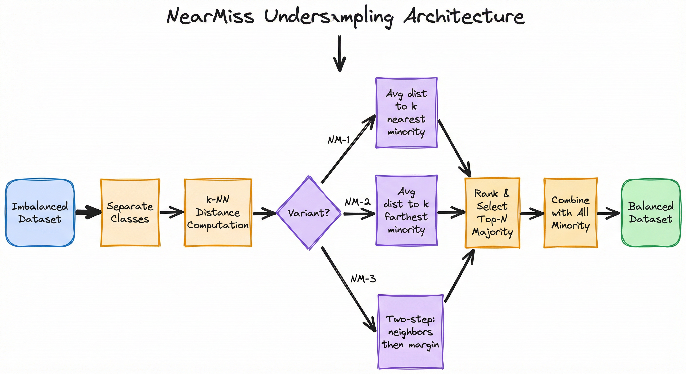
A flow diagram showing an imbalanced dataset being separated into classes, then processed through k-NN distance computation. The flow branches into three variant-specific paths (NearMiss-1 computing average distance to k nearest minority, NearMiss-2 computing average distance to k farthest minority, and NearMiss-3 using a two-step neighbors-then-margin approach). All paths converge to rank and select top-N majority samples, which are combined with all minority samples to produce a balanced dataset.
How to Implement
Implementation Approaches
NearMiss is primarily implemented via the imbalanced-learn (imblearn) library, which provides a unified API for all three variants through the version parameter. The library handles the k-NN distance computation internally using scikit-learn's NearestNeighbors, supporting multiple distance metrics and tree-based acceleration structures.
For production systems, NearMiss is applied as a preprocessing step in the training pipeline only — never at inference time. You undersample the training data, train your classifier on the balanced dataset, and deploy the classifier alone. The undersampled data is a training-time artifact.
Key configuration decisions: (1) Which variant to use — NearMiss-1 for aggressive boundary selection, NearMiss-2 for overlap-region focus, NearMiss-3 for safe margin selection. (2) The n_neighbors parameter (k) — typically 3 for small datasets, 5 for moderate, up to 10 for large. (3) The sampling_strategy — whether to fully balance to 1:1 or partially undersample to a target ratio.
Cost/Performance Note: NearMiss's k-NN search is computationally intensive for large majority classes. On a dataset with 1M majority samples and 10K minority samples, expect 2-5 minutes for NearMiss-1 on a 16-core CPU (AWS c6i.4xlarge, ~$0.68/hr or ~₹57/hr). NearMiss-3 is the most expensive due to its two-step process, typically taking 1.5-2x longer than NearMiss-1. The upside: the resulting balanced dataset is much smaller, so downstream model training is significantly faster.
from imblearn.under_sampling import NearMiss
from sklearn.datasets import make_classification
from sklearn.model_selection import train_test_split
from sklearn.ensemble import RandomForestClassifier
from sklearn.metrics import classification_report
import numpy as np

# Create imbalanced dataset (1:99 ratio)
X, y = make_classification(
    n_classes=2,
    weights=[0.01, 0.99],
    n_samples=10000,
    n_features=20,
    n_informative=10,
    random_state=42
)

print(f"Original class distribution: {np.bincount(y)}")
# Output: [100, 9900]

# Split data FIRST — never apply NearMiss before splitting
X_train, X_test, y_train, y_test = train_test_split(
    X, y, test_size=0.2, random_state=42, stratify=y
)

# Apply NearMiss-1 to training data only
nm1 = NearMiss(version=1, n_neighbors=3, sampling_strategy='auto')
X_train_resampled, y_train_resampled = nm1.fit_resample(X_train, y_train)

print(f"Resampled class distribution: {np.bincount(y_train_resampled)}")
# Output: [80, 80] — balanced by undersampling majority

print(f"Dataset reduced from {len(X_train)} to {len(X_train_resampled)} samples")
# Output: Dataset reduced from 8000 to 160 samples

# Train classifier on balanced data
clf = RandomForestClassifier(n_estimators=100, random_state=42)
clf.fit(X_train_resampled, y_train_resampled)

# Evaluate on original imbalanced test set
y_pred = clf.predict(X_test)
print(classification_report(y_test, y_pred))
This example demonstrates the standard NearMiss-1 workflow. Key points: (1) NearMiss is applied ONLY to the training set — never to the test set. (2) The version=1 parameter selects NearMiss-1, which keeps majority samples closest to minority neighbors. (3) With sampling_strategy='auto', the majority class is reduced to match the minority class size. (4) The dataset shrinks dramatically — from 8,000 to 160 samples — which means much faster training at the cost of losing majority class information.
from imblearn.under_sampling import NearMiss
from sklearn.datasets import make_classification
from sklearn.model_selection import train_test_split, cross_val_score
from sklearn.svm import SVC
from sklearn.preprocessing import StandardScaler
from imblearn.pipeline import Pipeline
import numpy as np

# Create imbalanced dataset
X, y = make_classification(
    n_classes=2,
    weights=[0.05, 0.95],
    n_samples=5000,
    n_features=15,
    n_informative=8,
    random_state=42
)

print(f"Class distribution: {np.bincount(y)}")
# Output: [250, 4750]

results = {}
for version in [1, 2, 3]:
    pipeline = Pipeline([
        ('scaler', StandardScaler()),
        ('nearmiss', NearMiss(
            version=version,
            n_neighbors=3,
            n_neighbors_ver3=3 if version == 3 else 3,
            sampling_strategy='auto'
        )),
        ('classifier', SVC(kernel='rbf', random_state=42))
    ])

    scores = cross_val_score(
        pipeline, X, y,
        cv=5,
        scoring='f1',
        n_jobs=-1
    )

    results[f'NearMiss-{version}'] = {
        'mean_f1': scores.mean(),
        'std_f1': scores.std()
    }
    print(f"NearMiss-{version}: F1 = {scores.mean():.3f} +/- {scores.std():.3f}")

# Typical output:
# NearMiss-1: F1 = 0.312 +/- 0.045
# NearMiss-2: F1 = 0.287 +/- 0.052
# NearMiss-3: F1 = 0.341 +/- 0.038
This example compares all three NearMiss variants using cross-validated F1 score with an SVM classifier. NearMiss-3 typically performs best because its two-step approach avoids selecting noisy boundary samples. NearMiss-1 can be overly aggressive, selecting majority samples that overlap with minority instances and creating a noisy training set. NearMiss-2 focuses on the overlap region, which can confuse the classifier. Note the use of imblearn.pipeline.Pipeline to ensure NearMiss is applied correctly within each cross-validation fold.
from imblearn.under_sampling import NearMiss
import numpy as np

# Suppose we have 50,000 majority, 500 minority samples
X = np.random.randn(50500, 20)
y = np.array([0]*50000 + [1]*500)

print(f"Original ratio (minority/majority): {500/50000:.4f}")
# Output: 0.0100

# Full balance to 1:1 (aggressive — loses 49,500 majority samples)
nm_full = NearMiss(version=1, n_neighbors=3, sampling_strategy='auto')
X_full, y_full = nm_full.fit_resample(X, y)
print(f"Full balance: {np.bincount(y_full)}")
# Output: [500, 500] — only 1000 total samples

# Partial balance to 1:5 ratio (preserves more information)
nm_partial = NearMiss(version=1, n_neighbors=3, sampling_strategy=0.2)
X_partial, y_partial = nm_partial.fit_resample(X, y)
print(f"Partial balance: {np.bincount(y_partial)}")
# Output: [2500, 500] — 3000 total samples

# Partial balance retains 5x more majority samples
print(f"Full balance kept {500/50000*100:.1f}% of majority samples")
print(f"Partial balance kept {2500/50000*100:.1f}% of majority samples")
# Output: Full kept 1.0%, Partial kept 5.0%
Setting sampling_strategy=0.2 targets a 1:5 minority-to-majority ratio instead of fully balancing to 1:1. This preserves more majority class information while still reducing the imbalance from 1:100 to 1:5. Partial undersampling is often a better practical choice than full balancing, especially when the majority class contains diverse patterns that would be lost with aggressive undersampling. You can then combine this with class weights in the downstream classifier to handle the remaining imbalance.
from imblearn.under_sampling import NearMiss
from sklearn.datasets import make_classification
from sklearn.model_selection import train_test_split
from sklearn.metrics import classification_report, roc_auc_score
from sklearn.linear_model import LogisticRegression
from sklearn.preprocessing import StandardScaler
import numpy as np

# Create noisy imbalanced dataset with class overlap
X, y = make_classification(
    n_classes=2,
    weights=[0.03, 0.97],
    n_samples=10000,
    n_features=15,
    n_informative=8,
    n_redundant=3,
    flip_y=0.05,  # 5% label noise
    class_sep=0.8,  # low class separation (overlap)
    random_state=42
)

X_train, X_test, y_train, y_test = train_test_split(
    X, y, test_size=0.2, stratify=y, random_state=42
)

scaler = StandardScaler()
X_train_scaled = scaler.fit_transform(X_train)
X_test_scaled = scaler.transform(X_test)

# NearMiss-3: two-step approach for noisy data
nm3 = NearMiss(
    version=3,
    n_neighbors=3,          # k for distance ranking in Step 2
    n_neighbors_ver3=5,     # m for neighbor identification in Step 1
    sampling_strategy='auto'
)
X_res, y_res = nm3.fit_resample(X_train_scaled, y_train)

print(f"Training set reduced: {len(X_train)} -> {len(X_res)} samples")
print(f"Class distribution: {np.bincount(y_res)}")

# Train logistic regression on clean balanced data
clf = LogisticRegression(max_iter=1000, random_state=42)
clf.fit(X_res, y_res)

y_pred = clf.predict(X_test_scaled)
y_prob = clf.predict_proba(X_test_scaled)[:, 1]

print(f"ROC-AUC: {roc_auc_score(y_test, y_prob):.3f}")
print(classification_report(y_test, y_pred))
NearMiss-3 is the best variant for noisy datasets with class overlap. The n_neighbors_ver3=5 parameter controls Step 1 (how many majority neighbors to keep around each minority sample), while n_neighbors=3 controls Step 2 (ranking by distance to nearest minority neighbors). By selecting majority samples that are near the minority class but not too close, NearMiss-3 avoids the noise amplification problem that plagues NearMiss-1 on overlapping datasets. Always scale features before applying NearMiss, as k-NN distance calculations are sensitive to feature magnitude.
# NearMiss-1 configuration (aggressive boundary selection)
nm1_config = {
    'version': 1,
    'n_neighbors': 3,                # k nearest minority neighbors
    'sampling_strategy': 'auto',     # balance to 1:1
    'n_jobs': -1                     # parallel distance computation
}

# NearMiss-2 configuration (overlap region focus)
nm2_config = {
    'version': 2,
    'n_neighbors': 5,                # k farthest minority neighbors
    'sampling_strategy': 0.3,        # target 0.3 minority/majority ratio
    'n_jobs': -1
}

# NearMiss-3 configuration (safe margin — recommended for production)
nm3_config = {
    'version': 3,
    'n_neighbors': 3,                # k for Step 2 ranking
    'n_neighbors_ver3': 5,           # m for Step 1 candidate selection
    'sampling_strategy': 'auto',
    'n_jobs': -1
}
Common Implementation Mistakes
- ●
Applying NearMiss before train-test split — This causes data leakage. The k-NN distance computation uses minority samples that might end up in the test set, biasing the selection of retained majority samples. ALWAYS split first, then apply NearMiss only to the training set.
- ●
Using NearMiss-1 on datasets with high class overlap — NearMiss-1 aggressively selects majority samples closest to minority instances. When classes overlap, this creates a training set dominated by ambiguous, potentially mislabeled samples near the boundary. Use NearMiss-3 instead, which maintains a safety margin.
- ●
Forgetting to scale features before NearMiss — k-NN distance calculations are scale-sensitive. If one feature ranges 0-100,000 (e.g., salary in INR) and another 0-1 (e.g., normalized age), the salary feature dominates all distance computations. Apply
StandardScalerorMinMaxScalerbefore NearMiss to ensure all features contribute equally. - ●
Full 1:1 balancing when partial undersampling would suffice — Undersampling to perfect 1:1 balance on a 1:1000 dataset discards 99.9% of majority samples. This extreme information loss often hurts more than it helps. Try
sampling_strategy=0.1or0.2first, then combine with class weights. - ●
Using NearMiss with very small minority classes (<30 samples) — When the minority class is tiny, the k-NN computation becomes unreliable because the "nearest neighbors" might still be far away. The retained majority samples may not actually be near a meaningful decision boundary. Collect more minority data or use cost-sensitive learning instead.
- ●
Not comparing NearMiss against random undersampling as a baseline — NearMiss is more computationally expensive than random undersampling due to the k-NN search. In some datasets, random undersampling performs equally well or better, making the computational overhead of NearMiss unjustified. Always compare.
When Should You Use This?
Use When
You have a large majority class (>100,000 samples) and need to reduce training set size for computational efficiency — NearMiss can cut training time by 10-100x by producing a much smaller balanced dataset
Your model struggles with class imbalance and oversampling (SMOTE) causes unacceptable increases in training time or memory consumption — NearMiss is the inverse approach that shrinks rather than grows the dataset
You want to preserve the original minority class exactly, without synthetic interpolation artifacts — NearMiss keeps all minority samples untouched while selecting a majority subset
The decision boundary between classes is the primary area of interest and interior majority samples add little value — NearMiss focuses retention on boundary-adjacent majority samples
You are building a quick prototype or baseline model where training speed matters more than preserving all majority class patterns — NearMiss + simple classifier can iterate much faster than full-dataset training
Features are predominantly continuous/numerical with meaningful distance metrics — NearMiss relies on k-NN distance, so features must support geometric distance computation
Avoid When
The majority class contains diverse subpopulations or patterns that would be lost by undersampling — NearMiss discards up to 99%+ of majority samples, potentially eliminating entire subgroups
Your dataset is already moderate in size (<10,000 total samples) — undersampling would reduce an already small dataset to dangerously few training samples, risking severe underfitting
Class overlap is minimal and the imbalance can be handled by simpler means like class weights or
scale_pos_weightin tree-based models — NearMiss adds unnecessary complexityFeatures are categorical or mixed-type — k-NN distance on categorical features is poorly defined, and NearMiss's distance-based selection becomes unreliable. Use random undersampling instead
You need a deterministic, auditable training process — NearMiss's k-NN selection can produce different results with different random seeds or distance metrics, complicating reproducibility audits in regulated domains
Precision is critical and you cannot afford any degradation — undersampling tends to reduce precision more than oversampling because the classifier loses the ability to model the majority class distribution accurately
Key Tradeoffs
The Core Tradeoff: Smaller Dataset vs Information Loss
NearMiss produces a dramatically smaller training set. On a dataset with 1M majority and 10K minority samples, NearMiss reduces the training set from 1.01M to 20K samples — a 50x reduction. This means 50x faster training, 50x less memory, and much faster experimentation cycles.
But that 50x reduction comes at a cost: 980K majority samples are permanently discarded. Those samples may contain valuable patterns, edge cases, or subpopulations that the model can no longer learn from. Unlike oversampling (which preserves all original data), undersampling is an irreversible information loss.
NearMiss vs Random Undersampling
| Aspect | NearMiss | Random Undersampling |
|---|---|---|
| Selection strategy | Distance-based (informed) | Uniform random |
| Boundary preservation | Excellent | Poor (random) |
| Computational cost | O(n_maj * n_min * d) | O(1) — constant |
| Reproducibility | Depends on k, metric, seed | Only depends on seed |
| Information retained | Boundary-focused | Representative of full distribution |
Surprisingly, random undersampling sometimes outperforms NearMiss in practice. This happens when the decision boundary is well-separated and the majority class distribution matters more than boundary details. Always compare both as baselines.
NearMiss vs SMOTE (Oversampling)
| Aspect | NearMiss (Undersampling) | SMOTE (Oversampling) |
|---|---|---|
| Dataset size | Smaller (faster training) | Larger (slower training) |
| Information loss | Discards majority samples | Preserves all original data |
| Synthetic artifacts | None | Possible (interpolation issues) |
| Precision impact | Often reduces precision | Moderate precision reduction |
| Best for | Large majority classes | Small minority classes |
Choosing Between NearMiss Variants
- NearMiss-1: Most aggressive boundary selection. Best for well-separated classes with clean labels. Worst for noisy data or overlapping classes.
- NearMiss-2: Selects majority samples near the core of the minority distribution. Best when classes overlap significantly and you want to model the overlap region.
- NearMiss-3: Safest choice. The two-step approach avoids selecting noise while still retaining boundary-informative samples. Recommended default for production.
Rule of Thumb: Start with NearMiss-3 for production systems. If you need faster computation and have clean data, try NearMiss-1. Use NearMiss-2 only when you specifically want to focus on the overlap region between classes. Always compare against random undersampling as a baseline — if random is equally good, prefer it for simplicity.
Alternatives & Comparisons
Random undersampling discards majority samples uniformly at random, without considering their position relative to the minority class. It is vastly faster (O(1) vs O(nmd) for NearMiss) and simpler to implement. Choose NearMiss when you specifically need boundary-focused undersampling and have clean, well-separated classes. Choose random undersampling when computational cost matters, when the majority class is homogeneous (no boundary advantage), or as a fast baseline before trying NearMiss.
Tomek Links is a cleaning technique that removes majority samples that form Tomek links with minority samples (pairs of nearest neighbors from different classes). Unlike NearMiss, which reduces the majority class to a target size, Tomek Links only removes ambiguous boundary pairs — typically removing far fewer samples. Choose Tomek Links for gentle boundary cleaning without aggressive undersampling. Choose NearMiss when you need substantial majority class reduction to balance the dataset.
Cluster Centroids replaces the majority class with cluster centroids generated by K-Means clustering, creating a synthetic compressed representation. Unlike NearMiss (which selects real samples), Cluster Centroids generates new representative points. Choose Cluster Centroids when you want a compact majority representation that preserves cluster structure. Choose NearMiss when you need to retain real, unmodified majority samples and want boundary-focused selection.
SMOTE is an oversampling technique that generates synthetic minority samples, while NearMiss is an undersampling technique that removes majority samples. They address imbalance from opposite directions. Choose SMOTE when you want to preserve all original data and have a small minority class. Choose NearMiss when the majority class is very large and you need to reduce training set size. In practice, combining NearMiss undersampling with SMOTE oversampling (a hybrid approach) often outperforms either technique alone.
Condensed Nearest Neighbour iteratively builds a minimal subset of the majority class that correctly classifies all samples using 1-NN. Like NearMiss, it is a prototype selection method, but CNN's selection criterion is classification accuracy rather than distance. Choose CNN when you want the smallest possible majority subset that preserves classification boundaries. Choose NearMiss when you want a specific target size and distance-based intuition for the selection.
Pros, Cons & Tradeoffs
Advantages
Reduces training set size dramatically, cutting training time and memory requirements by 10-100x for heavily imbalanced datasets — this translates to substantial cost savings on cloud compute (training on 20K samples instead of 1M can save ₹5,000-50,000 per run)
Preserves boundary-informative majority samples using distance-based selection, ensuring the model focuses on the decision boundary where classification decisions actually matter
No synthetic artifacts — unlike oversampling methods (SMOTE, ADASYN), NearMiss only selects real existing samples, avoiding interpolation issues with categorical features, discrete variables, or high-dimensional spaces
Three variants for different scenarios — NearMiss-1 for aggressive boundary focus, NearMiss-2 for overlap-region modeling, NearMiss-3 for safe margin selection with noise robustness
Simple and interpretable — the algorithm has clear geometric intuition (keep majority samples close to minority), making it easy to explain to stakeholders and audit in regulated domains
Well-integrated in Python ecosystem via imbalanced-learn, with scikit-learn-compatible API, pipeline support, and cross-validation integration through
imblearn.pipeline.PipelinePreserves all minority samples — the entire minority class is retained without modification, which is critical when minority samples are expensive or difficult to collect (e.g., rare disease cases, fraud examples)
Disadvantages
Irreversible information loss — discarding majority class samples permanently removes potentially valuable patterns, edge cases, and subpopulations that the model can no longer learn from
k-NN computation is expensive for large datasets — computing pairwise distances between majority and minority samples scales as , which can take minutes for million-sample datasets
NearMiss-1 can create noisy training sets by selecting majority samples that overlap with minority instances, especially when classes are not well-separated or labels contain errors
Often reduces precision more than oversampling methods, because the classifier loses its ability to model the majority class distribution accurately with so few majority samples
Sensitive to feature scaling — distance-based selection produces different results depending on feature normalization, requiring careful preprocessing that may not always be straightforward
May underperform random undersampling on some datasets — the computational overhead of k-NN-based selection is not always justified, especially when the decision boundary is well-separated or the majority class is homogeneous
Struggles with high-dimensional data due to the curse of dimensionality — in high dimensions, distances between all points converge, making nearest-neighbor selection less meaningful and reducing NearMiss's advantage over random selection
Failure Modes & Debugging
Catastrophic majority class information loss
Cause
Full 1:1 balancing on extremely imbalanced datasets (e.g., 1:1000) discards 99.9% of majority samples. The retained 0.1% may not represent the true majority class distribution, causing the classifier to misunderstand the majority class entirely.
Symptoms
High recall for minority class but extremely low precision. The model over-predicts the minority class because it has lost the ability to recognize diverse majority patterns. In production, the model generates excessive false positives (e.g., flagging legitimate transactions as fraud at a 50%+ rate).
Mitigation
Use partial undersampling with sampling_strategy=0.1 or 0.2 instead of full 1:1 balancing. Combine NearMiss with class weights in the downstream classifier to handle remaining imbalance. Consider hybrid approaches (NearMiss + SMOTE) that partially reduce the majority while partially increasing the minority. Set a minimum threshold for retained majority samples (e.g., never discard more than 90% of majority data).
Noisy boundary selection with NearMiss-1
Cause
NearMiss-1 selects majority samples closest to minority neighbors. When classes overlap or labels contain errors, the closest majority samples are often in the overlap zone — the noisiest, most ambiguous region. The resulting training set is dominated by difficult-to-classify, potentially mislabeled samples.
Symptoms
Model performance is worse with NearMiss-1 than with random undersampling. Training accuracy is low even on the undersampled dataset. The model exhibits high variance across different random seeds. Visual inspection shows retained majority samples clustering tightly around minority samples with no clear separation.
Mitigation
Switch to NearMiss-3, which uses a two-step approach to avoid selecting majority samples that are too close to minority instances. Apply outlier detection (Isolation Forest, LOF) to remove noisy samples before NearMiss. Increase n_neighbors (k) to smooth out the distance computation and reduce sensitivity to individual noisy points. Consider Tomek Links for gentle boundary cleaning instead of aggressive boundary selection.
Distance metric failure in high-dimensional spaces
Cause
In high-dimensional feature spaces (>100 features), Euclidean distances between all points converge to similar values (the curse of dimensionality). NearMiss's distance-based selection becomes essentially random because the "nearest" and "farthest" neighbors have nearly identical distances.
Symptoms
NearMiss performs no better than random undersampling despite the computational overhead. Increasing k has negligible effect on the selected subset. The distance distribution for majority samples is tightly concentrated, with minimal spread between the closest and farthest minority neighbors.
Mitigation
Apply dimensionality reduction (PCA, UMAP, autoencoders) before NearMiss to reduce features to 10-30 meaningful dimensions. Use Manhattan distance ( norm) or cosine distance instead of Euclidean, as these are more robust in high dimensions. Alternatively, abandon distance-based undersampling and use random undersampling or cluster-based methods (Cluster Centroids) that are less sensitive to dimensionality.
Minority subpopulation blind spots
Cause
NearMiss selects majority samples based on proximity to the minority class as a whole. If the minority class has multiple distinct subpopulations (clusters), NearMiss may concentrate retained majority samples near the largest minority cluster while ignoring smaller clusters entirely.
Symptoms
High recall on the dominant minority subpopulation but near-zero recall on smaller minority subgroups. For example, in fraud detection, the model catches common fraud patterns but misses rare fraud types. Cross-validation shows high variance in minority class recall across folds.
Mitigation
Apply NearMiss separately to each minority subpopulation (first cluster the minority class using K-Means or DBSCAN, then apply NearMiss per cluster). Use stratified sampling within NearMiss by controlling the selection to proportionally represent different minority regions. Consider ensemble approaches where multiple NearMiss models are trained on different undersampled subsets.
Computational timeout on large-scale datasets
Cause
k-NN distance computation between all majority-minority pairs scales as O(n_maj * n_min * d). For datasets with millions of majority samples and thousands of minority samples, this can take hours even with optimized implementations.
Symptoms
NearMiss preprocessing step dominates pipeline runtime (>30 minutes). Memory usage spikes during distance computation. Pipeline times out in CI/CD or scheduled training jobs. CPU utilization at 100% for extended periods.
Mitigation
Subsample the majority class randomly before applying NearMiss (e.g., first random undersample from 1M to 50K, then apply NearMiss to select 10K). Use approximate nearest neighbor algorithms (Annoy, FAISS) for the distance computation. Increase n_jobs for parallel computation. For very large datasets (>10M), use random undersampling instead — the computational cost of NearMiss is rarely justified at this scale.
Placement in an ML System
NearMiss sits in the data preprocessing stage of the ML pipeline, specifically after data cleaning, feature extraction, and train-test split, but before model training. It is strictly a training-time technique — the undersampled dataset is used only for training, never for inference or evaluation.
Upstream dependencies: NearMiss requires clean, numerical features with meaningful distance metrics. Categorical variables should be encoded (target encoding, embeddings, or one-hot) before applying NearMiss, as k-NN distance on raw categoricals is undefined. Features should be scaled (StandardScaler, MinMaxScaler) since k-NN is distance-sensitive — unscaled features with different magnitudes will bias the selection toward high-variance features. Outliers should be addressed before NearMiss, as noisy minority samples will attract incorrect majority selections.
Downstream impact: The undersampled dataset produced by NearMiss feeds directly into model training. Because the dataset is dramatically smaller (sometimes 50-100x), training is much faster and requires less memory. However, the classifier must compensate for the lost majority class information — this often means the model has higher recall but lower precision on the minority class compared to training on the full dataset.
Pipeline integration: NearMiss should be integrated via imblearn.pipeline.Pipeline to ensure correct application during cross-validation (only to training folds, never validation folds). In production training pipelines, NearMiss is applied as a preprocessing step that runs before the training loop. The undersampled indices should be logged for auditability.
Production considerations: In production, NearMiss is applied during model training only. The deployed model receives real-world data at inference time — no undersampling occurs during serving. This means NearMiss has zero runtime overhead in production. However, the training pipeline must be carefully monitored: if the minority class distribution shifts over time (data drift), the NearMiss selection may become stale, requiring retraining with fresh undersampling.
Pipeline Stage
Data Preprocessing / Training
Upstream
- data-cleaning
- data-validation
- feature-extraction
- train-test-split
Downstream
- model-training
- hyperparameter-tuning
- cross-validation
Scaling Bottlenecks
NearMiss's k-NN search is the primary bottleneck at scale. For majority classes with >100,000 samples, the pairwise distance computation can take 5-15 minutes on a modern multi-core CPU. Unlike SMOTE (which scales with minority class size), NearMiss's cost grows linearly with majority class size — precisely the dimension that is large in imbalanced datasets. Memory consumption scales as O(n_maj * k) for storing distance vectors. At extreme scale (10M+ majority samples), the k-NN search can take hours even with KD-tree acceleration, making random undersampling or cluster-based methods more practical. For datasets with high dimensionality (>100 features), KD-trees degrade to naive O(n^2) performance, exacerbating the bottleneck.
Production Case Studies
A comprehensive study on credit card fraud detection evaluated multiple resampling techniques including NearMiss, SMOTE, and random undersampling on the Kaggle Credit Card Fraud Dataset (284,807 transactions, 0.17% fraud). NearMiss-1 was used to undersample the legitimate transaction class, retaining majority samples closest to fraudulent transactions for training various classifiers including Random Forest and XGBoost.
NearMiss-1 combined with Random Forest achieved 89% accuracy with improved recall for fraud detection, though it underperformed SMOTE-based oversampling (99% accuracy). The study concluded that NearMiss is effective for rapid prototyping but hybrid approaches (NearMiss + SMOTE) are preferred for production fraud detection where both precision and recall are critical.
Researchers applied NearMiss undersampling to imbalanced COVID-19 county-level severity datasets where severe cases were vastly outnumbered by mild cases. NearMiss was used to create balanced training sets for ensemble classifiers predicting disease severity from demographic and health indicators across US counties.
NearMiss undersampling combined with ensemble learning demonstrated superior capability in predicting COVID-19 severity levels, achieving balanced accuracy of 78-85% compared to 62% without resampling. The approach was particularly effective at identifying high-risk counties with limited severe case data.
A detailed study evaluated NearMiss alongside random undersampling and Tomek Links for classifying cyberattacks in the CICIDS2017 intrusion detection dataset. The dataset is heavily imbalanced with benign traffic vastly outnumbering attack categories. NearMiss-1 was used to reduce the benign traffic class while preserving attack-adjacent samples.
NearMiss-1 achieved balanced trade-offs in precision (82%), recall (87%), F1 score (84%), and AUC (0.91) for minority attack classes, outperforming random undersampling on rare attack categories. However, Tomek Links provided better precision when combined with oversampling, suggesting NearMiss is most effective as part of a hybrid pipeline.
Researchers compared SMOTE and NearMiss methods for disease classification using the Indonesian Family Life Survey (IFLS 5) dataset, which has significant class imbalance in disease prevalence. NearMiss was applied to undersample healthy individuals to match the number of disease-positive cases for training classification models across multiple disease categories.
NearMiss-based models achieved 73-81% recall for rare diseases, compared to 45-58% without resampling. However, SMOTE outperformed NearMiss on overall F1 score (0.79 vs 0.71) due to better precision preservation. The study recommended combining NearMiss with SMOTE for optimal performance on highly imbalanced health survey data.
Tooling & Ecosystem
The canonical Python library for NearMiss and all imbalanced learning techniques. Provides NearMiss class with version parameter (1, 2, or 3), n_neighbors, n_neighbors_ver3, and sampling_strategy. Fully compatible with scikit-learn pipelines via imblearn.pipeline.Pipeline. Version 0.14.1 as of 2026, actively maintained by scikit-learn-contrib.
While scikit-learn does not include NearMiss directly, it provides the NearestNeighbors class that powers NearMiss's distance computation, along with the pipeline and cross-validation infrastructure that NearMiss integrates with. Also offers sklearn.utils.resample for basic random undersampling as a simpler alternative.
R implementation of NearMiss as a recipe step (step_nearmiss) in the tidymodels ecosystem. Integrates with the recipes package for preprocessing workflows. Supports all three NearMiss variants and provides a familiar tidyverse-style API for R users working with imbalanced datasets.
High-performance library for efficient similarity search and nearest neighbor computation. While not a NearMiss implementation itself, FAISS can dramatically accelerate the k-NN distance computation that NearMiss relies on, especially for large datasets (>1M samples) where scikit-learn's NearestNeighbors becomes a bottleneck. GPU-accelerated variant available.
Spotify's approximate nearest neighbors library, useful for scaling NearMiss's k-NN computation to large datasets. Trades exact distance computation for speed (typically 10-100x faster with >95% recall). Can be used as a drop-in replacement for the exact k-NN search when NearMiss's O(n^2) computation is prohibitive.
Research & References
Mani, I., Zhang, I. (2003)Proceedings of Workshop on Learning from Imbalanced Datasets, ICML 2003
The original NearMiss paper introducing three distance-based undersampling variants for handling class imbalance. Demonstrated that NearMiss methods outperform random undersampling on information extraction tasks by retaining majority samples near the decision boundary. Established the foundation for heuristic undersampling in imbalanced learning.
Batista, G.E.A.P.A., Prati, R.C., Monard, M.C. (2004)ACM SIGKDD Explorations Newsletter, vol. 6, issue 1
Comprehensive comparison of oversampling (SMOTE) and undersampling (random, NearMiss, Tomek Links, CNN) methods across 13 UCI datasets. Found that hybrid approaches combining SMOTE with Tomek Links or ENN outperform pure undersampling or oversampling alone. Showed NearMiss-1 can be overly aggressive on noisy datasets while NearMiss-3 provides more robust selection.
Boateng, R., Kudjo, P.K., Mensah, S. (2024)PeerJ Computer Science
Evaluated five undersampling methods (random, NearMiss, cluster centroids, repeated edited nearest neighbor, Tomek Links) and three oversampling methods for cyberattack classification. Found NearMiss achieved balanced trade-offs across precision, recall, F1, and AUC, outperforming other undersampling strategies on rare attack categories in the CICIDS2017 dataset.
Fernandez, A., Garcia, S., Galar, M., et al. (2024)Artificial Intelligence Review
Comprehensive survey of imbalanced learning techniques in healthcare over 2014-2024. Found that undersampling methods including NearMiss are widely used in medical AI, appearing in 22% of surveyed papers as a preprocessing step. Highlighted that NearMiss combined with ensemble methods (bagging, boosting) achieves robust performance on small medical datasets where oversampling risks overfitting.
More, A.S., Rana, D.P. (2017)arXiv preprint
Broad survey covering resampling techniques including NearMiss, SMOTE, random sampling, and hybrid methods. Provides empirical comparison of NearMiss variants showing NearMiss-3 generally outperforms NearMiss-1 and NearMiss-2 due to its two-step noise-resistant approach. Recommended NearMiss for moderate imbalance ratios (1:10 to 1:100) but cautioned against its use for extreme imbalance (>1:1000).
Interview & Evaluation Perspective
Common Interview Questions
- ●
Explain the three NearMiss variants and when you would choose each one
- ●
What is the difference between NearMiss and random undersampling? When does each perform better?
- ●
How does NearMiss compare to SMOTE for handling class imbalance?
- ●
What are the failure modes of NearMiss and how would you mitigate them?
- ●
When would you choose undersampling over oversampling for an imbalanced dataset?
- ●
How would you implement NearMiss correctly in a cross-validation pipeline?
- ●
What happens to NearMiss performance in high-dimensional feature spaces?
- ●
Describe a scenario where NearMiss would hurt model performance instead of helping
Key Points to Mention
- ●
NearMiss is a family of three distance-based undersampling methods that select majority samples based on proximity to minority instances using k-NN
- ●
NearMiss-1 selects majority samples with smallest average distance to k nearest minority neighbors (aggressive boundary focus)
- ●
NearMiss-2 selects majority samples with smallest average distance to k farthest minority neighbors (overlap region focus)
- ●
NearMiss-3 uses a two-step approach: first finds majority neighbors of minority samples, then selects those with largest distance to k nearest minority neighbors (safe margin)
- ●
Key trade-off is information loss vs dataset reduction — NearMiss can discard 99%+ of majority samples, dramatically reducing training time but potentially losing valuable patterns
- ●
Must be applied ONLY to training data after train-test split to avoid data leakage through the k-NN distance computation
- ●
Features must be scaled before NearMiss since k-NN distance is scale-sensitive — unscaled features bias the selection
- ●
NearMiss-3 is generally recommended for production because it avoids selecting noisy boundary samples
Pitfalls to Avoid
- ●
Claiming NearMiss is always better than random undersampling — random sometimes matches or beats NearMiss with much less computational cost
- ●
Applying NearMiss before train-test split, which leaks information through the k-NN distance computation
- ●
Ignoring that full 1:1 balancing on extreme imbalance ratios (>1:100) can destroy the majority class representation
- ●
Forgetting feature scaling, which completely changes which majority samples are selected
- ●
Not mentioning the computational cost — NearMiss is O(n_maj * n_min * d), which can be prohibitive for large datasets
- ●
Using NearMiss-1 on noisy data without acknowledging it selects the most ambiguous, potentially mislabeled samples
Senior-Level Expectation
Senior/staff-level candidates should demonstrate understanding of NearMiss beyond the textbook algorithm. Discuss the trade-off between NearMiss's boundary-focused selection and the risk of losing majority class diversity. Compare NearMiss against the full landscape of imbalance-handling techniques: random undersampling (simpler, sometimes equally effective), SMOTE (preserves all data but increases size), class weights (no data modification), focal loss (algorithm-level solution), and ensemble methods (EasyEnsemble, BalanceCascade). Show awareness that NearMiss-3 is generally safest for production due to its noise-resistant two-step approach. Discuss computational scaling: for million-sample datasets, NearMiss's k-NN search is a real bottleneck, and approximate nearest neighbor libraries (FAISS, Annoy) may be needed. Ideally, share a real production experience: 'We tried NearMiss-1 on our fraud detection pipeline but it created too many false positives because it selected the noisiest boundary samples. We switched to NearMiss-3 with partial undersampling (1:5 ratio) combined with XGBoost class weights, which improved minority recall from 68% to 83% while keeping precision above 75%.'
Summary
NearMiss is a family of distance-based undersampling techniques that address class imbalance by intelligently selecting which majority class samples to retain based on their proximity to minority class instances. Introduced by Mani and Zhang in 2003, it offers three variants: NearMiss-1 (keep majority samples closest to nearest minority neighbors), NearMiss-2 (keep majority samples closest to farthest minority neighbors), and NearMiss-3 (a two-step approach that selects majority samples near the minority class but not too close, creating a safe margin). NearMiss-3 is generally recommended for production use due to its robustness to noise and label errors.
The technique's primary advantage is dramatic dataset reduction — on heavily imbalanced datasets, NearMiss can shrink the training set by 50-100x, cutting training time and compute costs proportionally. For Indian fintech companies processing millions of transactions, this can translate to savings of ₹15,000+ per month on training pipelines. Unlike oversampling methods like SMOTE, NearMiss produces no synthetic artifacts, preserves all minority samples, and generates smaller training sets that are faster to iterate with.
However, NearMiss comes with significant tradeoffs. The irreversible loss of majority class information can degrade precision and eliminate diverse majority patterns. NearMiss-1, in particular, can create noisy training sets by selecting the most ambiguous boundary samples. The k-NN distance computation adds preprocessing overhead that scales as O(n_maj * n_min * d), and in high-dimensional spaces, distance-based selection loses its advantage over random undersampling due to the curse of dimensionality.
Modern best practice treats NearMiss as one tool in a broader imbalance-handling toolkit. For tree-based models (XGBoost, Random Forest), native class weights often outperform NearMiss without the information loss. For SVMs and k-NN classifiers, NearMiss's boundary-focused selection provides genuine improvement. The most robust production approach is often hybrid: NearMiss for moderate majority reduction (1:100 to 1:10), SMOTE for moderate minority expansion (1:10 to 1:3), and class weights for the remaining imbalance. This balances information preservation, computational efficiency, and classification performance across domains from fraud detection to medical diagnosis to intrusion detection.