Audio Augmentation in Machine Learning
Audio augmentation is the practice of applying label-preserving transformations to audio signals -- time stretching, pitch shifting, noise injection, room simulation, spectral masking -- to expand training data and make models robust to the acoustic conditions they will face in the real world.
If you have ever talked to a voice assistant in a noisy kitchen, on a crowded Mumbai local, or in a reverberant conference hall, you have experienced the problem audio augmentation solves. The model that transcribes your speech was almost certainly trained on clean studio recordings. Without augmentation, it would fail catastrophically in any of those environments. Audio augmentation bridges the gap between lab-quality training data and the messy acoustics of production deployment.
What makes audio augmentation distinct from image or text augmentation is the dual-domain nature of audio data. You can augment in the time domain (directly manipulating the waveform -- adding noise, shifting pitch, stretching time) or in the frequency domain (masking spectrogram bands, warping spectral features). The landmark SpecAugment paper from Google showed that frequency-domain augmentation alone could push ASR systems to state-of-the-art performance with zero changes to the model architecture.
Today, audio augmentation is non-negotiable in production speech and sound recognition systems. Google uses it in every Assistant-powered device. OpenAI's Whisper large-v2 added SpecAugment to its training pipeline after the initial release. Indian startups like Sarvam AI augment extensively to handle the acoustic diversity of 22 official languages spoken across wildly different environments. Whether you are building an ASR system, a music classifier, a speaker verification model, or an environmental sound detector, understanding audio augmentation is foundational.
This guide covers everything: the core techniques (time-domain and frequency-domain), the mathematical foundations, production-grade implementation with audiomentations and torchaudio, failure modes that silently degrade your models, and the decision framework for choosing which augmentations to apply.
Concept Snapshot
- What It Is
- A collection of signal processing techniques that apply label-preserving transformations to audio waveforms and spectrograms, creating synthetic training variations that improve model robustness to real-world acoustic conditions without collecting additional labeled data.
- Category
- Data Generation
- Complexity
- Intermediate
- Inputs / Outputs
- Inputs: raw audio waveforms (WAV, FLAC, MP3) or their spectrogram representations (mel-spectrograms, MFCCs) with labels. Outputs: augmented audio/spectrograms with the same labels, effectively multiplying dataset diversity.
- System Placement
- Applied during the data loading/preprocessing stage of the training pipeline, after audio decoding but before feature extraction or model input. Some augmentations (SpecAugment) are applied after feature extraction, directly on spectrograms.
- Also Known As
- speech augmentation, audio data augmentation, acoustic augmentation, waveform augmentation, spectral augmentation
- Typical Users
- Speech engineers, ML engineers, Audio ML researchers, ASR developers, Sound classification engineers, Music information retrieval researchers
- Prerequisites
- Basic signal processing (sampling rate, Fourier transform), Understanding of spectrograms and mel-frequency features, Familiarity with deep learning training pipelines, Python and PyTorch/TensorFlow basics
- Key Terms
- time stretchingpitch shiftingspeed perturbationSpecAugmentnoise injectionroom impulse responsefrequency maskingtime maskingaudio mixupmel-spectrogramSTFTreverberation
Why This Concept Exists
The Acoustic Mismatch Problem
Here is the fundamental challenge: training audio is collected in controlled conditions, but models deploy into acoustic chaos. A speech recognition model trained on LibriSpeech (read English from audiobooks in quiet rooms) encounters traffic noise on Delhi roads, reverberant temple halls in Tirupati, crowded wedding mandaps, and the tinny speaker of a budget Android phone. Without augmentation, the model's word error rate can double or triple in these conditions.
This mismatch is more severe in audio than in vision or text. A photo taken in a different room still looks like a photo. But audio recorded in a different room sounds fundamentally different -- reverberation changes the temporal structure of speech, background noise masks phonemes, and microphone characteristics colour the frequency response. The acoustic environment is not just context; it is part of the signal itself.
The Cost of Diverse Audio Data
Collecting acoustically diverse training data is prohibitively expensive. To properly cover the range of real-world conditions, you would need recordings in quiet rooms, noisy cafes, moving vehicles, open fields, reverberant halls, and more -- for every speaker, every language, every accent. For a 1,000-hour ASR dataset (a modest size by modern standards), recording in 10 acoustic environments would require 10,000 hours of studio time, costing upwards of $500,000 (approximately 4.2 crore INR). Most teams cannot afford this.
Augmentation offers a compelling alternative: simulate acoustic diversity computationally at near-zero marginal cost. Adding background noise from the MUSAN corpus, convolving with room impulse responses (RIRs), and applying speed perturbation can transform 1,000 hours of clean speech into 5,000-10,000 hours of acoustically diverse training data in a few hours of CPU time.
The SpecAugment Revolution
Before 2019, audio augmentation was primarily done in the time domain -- adding noise, changing speed, shifting pitch. Then Google published SpecAugment (Park et al., 2019), which applied augmentation directly to the spectrogram representation: masking blocks of frequency channels and time steps. This absurdly simple technique -- essentially blacking out rectangles on the spectrogram -- reduced the word error rate on LibriSpeech test-other from 12.5% to 6.8%, a massive improvement with zero architectural changes.
SpecAugment changed the field's understanding of augmentation. It showed that even destroying information (masking parts of the input) forces models to learn more robust representations, relying on context rather than memorizing specific spectral patterns. This is analogous to dropout, but applied to the input rather than hidden layers.
The Indian Language Imperative
India presents a uniquely challenging audio landscape. With 22 official languages, hundreds of dialects, and a population that increasingly interacts with technology via voice (thanks to JioPhone, Google Assistant in Hindi, and voice-first apps like Kuku FM and Pratilipi), robust audio ML is critical. But labeled speech data for languages like Odia, Assamese, or Maithili is scarce -- sometimes under 100 hours. Audio augmentation is the primary strategy for stretching these limited resources. Projects like Vakyansh (ASR toolkit for 18 Indic languages) and Sarvam AI rely heavily on augmentation to achieve production-quality recognition across India's linguistic diversity.
Key Takeaway: Audio augmentation exists because real-world acoustics are infinitely variable, diverse audio collection is prohibitively expensive, and simple augmentation techniques like SpecAugment and noise injection deliver dramatic improvements in model robustness at near-zero cost.
Core Intuition & Mental Model
The Core Promise
Audio augmentation guarantees this: if a transformation does not change what is being said (or what sound is being made), applying that transformation during training will make the model more robust to encountering similar variations at inference time.
Time-stretch a speech clip by 10% and the words are the same, just spoken slightly slower. Add cafeteria noise at 15 dB SNR and the words are still audible, just harder to hear. Convolve with a room impulse response and the words echo slightly, but remain the same. In each case, a human listener would assign the same transcription -- so the label is preserved.
The Two Domains
What makes audio augmentation unique is that you can operate in two complementary domains:
Time-domain augmentation manipulates the raw waveform directly. Think of it as physically altering the recording: adding background noise (mixing signals), stretching time (resampling), shifting pitch (modulating frequency), or simulating room acoustics (convolution with impulse responses). These augmentations have clear physical interpretations -- you are simulating a noisier room, a different speaker's pitch, or a larger hall.
Frequency-domain augmentation manipulates the spectrogram (the time-frequency representation). SpecAugment is the canonical example: it masks random blocks of frequency bands or time steps, forcing the model to make predictions from incomplete information. This has no direct physical analogue -- you are not simulating a real-world condition, but rather teaching the model to be resilient to missing information, much like dropout teaches neural networks not to rely on any single neuron.
The best production pipelines combine both: time-domain augmentation to simulate real acoustic conditions, and frequency-domain augmentation to regularize the model.
The Analogy: Teaching a Child in Noisy Classrooms
Imagine teaching a child to recognize spoken words. If the child only ever hears speech in a silent room, they will struggle in a busy bazaar. But if you gradually introduce background noise -- first soft traffic sounds, then crowd chatter, then music -- the child learns to focus on the speech signal and filter out distractions. That is exactly what noise injection does for an ML model.
Similarly, if the child only hears one speaker (say, their teacher), they might struggle with a different voice. Speed perturbation and pitch shifting simulate hearing the same words from speakers with different vocal characteristics, teaching the model to focus on what is said rather than who is saying it.
Mental Model: Audio augmentation is acoustic stress-testing during training. You deliberately degrade, distort, and diversify the audio signal to build a model that thrives in imperfect conditions. The goal is not to create realistic audio, but to create useful training variations that force the model to learn robust representations.
Technical Foundations
Mathematical Framework
Intuition First: You have a dataset of (audio, label) pairs. Augmentation applies transformations to audio signals while keeping labels unchanged, creating a larger and more diverse effective training set.
Formally: Let be a training set where is a discrete-time audio signal of length samples and is its label (transcription, class, speaker ID, etc.). An augmentation function transforms the signal while preserving label semantics.
Time-Domain Augmentations
Speed Perturbation (Ko et al., 2015): Resample the signal at a different rate to change speaking speed:
where is the speed factor (typically ). This changes both tempo and pitch simultaneously. The output length is .
Time Stretching: Modify duration without changing pitch using the phase vocoder algorithm. The Short-Time Fourier Transform (STFT) is computed, phases are interpolated, and the inverse STFT reconstructs the stretched signal:
where is the stretch factor. Unlike speed perturbation, pitch is preserved: but (fundamental frequency) stays constant.
Pitch Shifting: Modify pitch without changing duration by combining time stretching with resampling:
where is the shift in semitones. Typical range: semitones.
Additive Noise Injection: Mix the signal with a noise signal at a target signal-to-noise ratio (SNR):
where and are the power of signal and noise respectively. Typical SNR range: 5-20 dB.
Room Impulse Response (RIR) Convolution: Simulate room acoustics by convolving with an impulse response :
where is the RIR capturing reflections, absorption, and diffusion of a room. The direct path determines the dry/wet ratio.
Frequency-Domain Augmentations (SpecAugment)
Frequency Masking: Given a mel-spectrogram with frequency bins, mask consecutive frequency channels starting at :
where and .
Time Masking: Analogously, mask consecutive time steps starting at :
where .
Audio Mixup
Extend the Mixup principle to audio: given two samples and :
where . For ASR, MixSpeech operates on spectrograms and uses the mixing coefficient to weight both transcription losses.
Important: Speed perturbation simultaneously changes tempo and pitch (coupling the two), while time stretching decouples them. For ASR, speed perturbation is preferred because the resulting pitch+tempo co-variation mimics natural speaker variability. For music tasks, independent control via time stretching + pitch shifting is usually necessary.
Internal Architecture
A production audio augmentation pipeline operates across two stages: waveform-level augmentation (before feature extraction) and spectrogram-level augmentation (after feature extraction). This dual-stage design maximizes diversity while keeping compute overhead manageable.
The waveform stage handles physically interpretable transforms: noise injection, RIR convolution, speed perturbation, and pitch shifting. These simulate real-world acoustic conditions. The spectrogram stage applies SpecAugment-family transforms: frequency masking, time masking, and time warping. These act as regularizers without physical analogue.
For on-the-fly training, augmentations are applied randomly per sample in the data loader's collation step. This ensures the model sees different augmented variants each epoch, providing infinite effective diversity. The augmentation policy (which transforms, their probabilities, and parameter ranges) is typically defined in a YAML config for reproducibility.
Key Components
Audio Decoder
Loads raw audio files (WAV, FLAC, MP3, OGG) and converts them to float32 tensors at the target sample rate. Handles resampling if the source sample rate differs from the target (e.g., 44.1 kHz to 16 kHz for speech). Implementations: torchaudio.load(), soundfile.read(), librosa.load().
Waveform Augmenter
Applies time-domain transformations to the raw audio signal. Orchestrates a chain of augmentations (noise injection, speed perturbation, pitch shift, RIR convolution, gain adjustment, clipping simulation) with configurable probabilities and parameter ranges. Libraries: audiomentations, WavAugment, torch-audiomentations.
Noise Injection Module
Mixes background noise from a noise corpus (MUSAN, AudioSet, custom recordings) into the audio at a random SNR. Supports multiple noise types: Gaussian white noise, environmental noise (traffic, crowd, rain), music, and babble speech. The SNR is sampled uniformly from a configured range (typically 5-20 dB).
Room Simulator
Convolves audio with Room Impulse Responses (RIRs) to simulate reverberant environments. Uses pre-recorded RIRs (openSLR-28 dataset) or synthetically generated ones (via pyroomacoustics). Controls dry/wet mix ratio to adjust reverberation intensity.
Feature Extractor
Converts augmented waveforms to spectral features: mel-spectrograms, MFCCs, filter banks, or raw STFT magnitudes. Parameters: FFT size (typically 512 or 1024), hop length (160 or 256), number of mel bands (80 or 128). Implementations: torchaudio.transforms.MelSpectrogram, librosa.feature.melspectrogram.
SpecAugment Module
Applies frequency-domain augmentation to spectrograms: frequency masking (zeroing random horizontal bands), time masking (zeroing random vertical bands), and optional time warping. Operates on the spectrogram tensor in-place. Parameters: max frequency mask width , max time mask width , number of masks and . Implemented in torchaudio.transforms.FrequencyMasking and torchaudio.transforms.TimeMasking.
Augmentation Policy Manager
Stores the full augmentation configuration: which transforms to apply, their probabilities, parameter ranges, and sequencing. Ensures reproducibility by supporting random seed control. Typically defined in YAML or JSON config files, allowing easy experimentation with different policies.
Data Flow
Here is the typical data flow in a production pipeline:
Training Path: Audio file loaded from disk (WAV/FLAC, 16 kHz, mono) --> Waveform augmentation chain (speed perturbation with factor sampled from {0.9, 1.0, 1.1}, then noise injection at SNR 5-20 dB with 50% probability, then RIR convolution with 30% probability) --> Feature extraction (80-dim mel-spectrogram, 25ms window, 10ms hop) --> SpecAugment (2 frequency masks of width up to 27, 2 time masks of width up to 100) --> Batch collation with padding --> Model input.
Inference Path (Standard): Audio file loaded --> Feature extraction (same parameters as training, no augmentation) --> Model inference --> Prediction.
Inference Path (Test-Time Augmentation): Audio file loaded --> Generate K augmented variants (original, +noise at 15 dB, speed 0.95, speed 1.05) --> Feature extraction on each --> Model inference on each --> Ensemble predictions (average logits or vote) --> Final prediction. Rare in audio compared to vision, but used in Kaggle competitions.
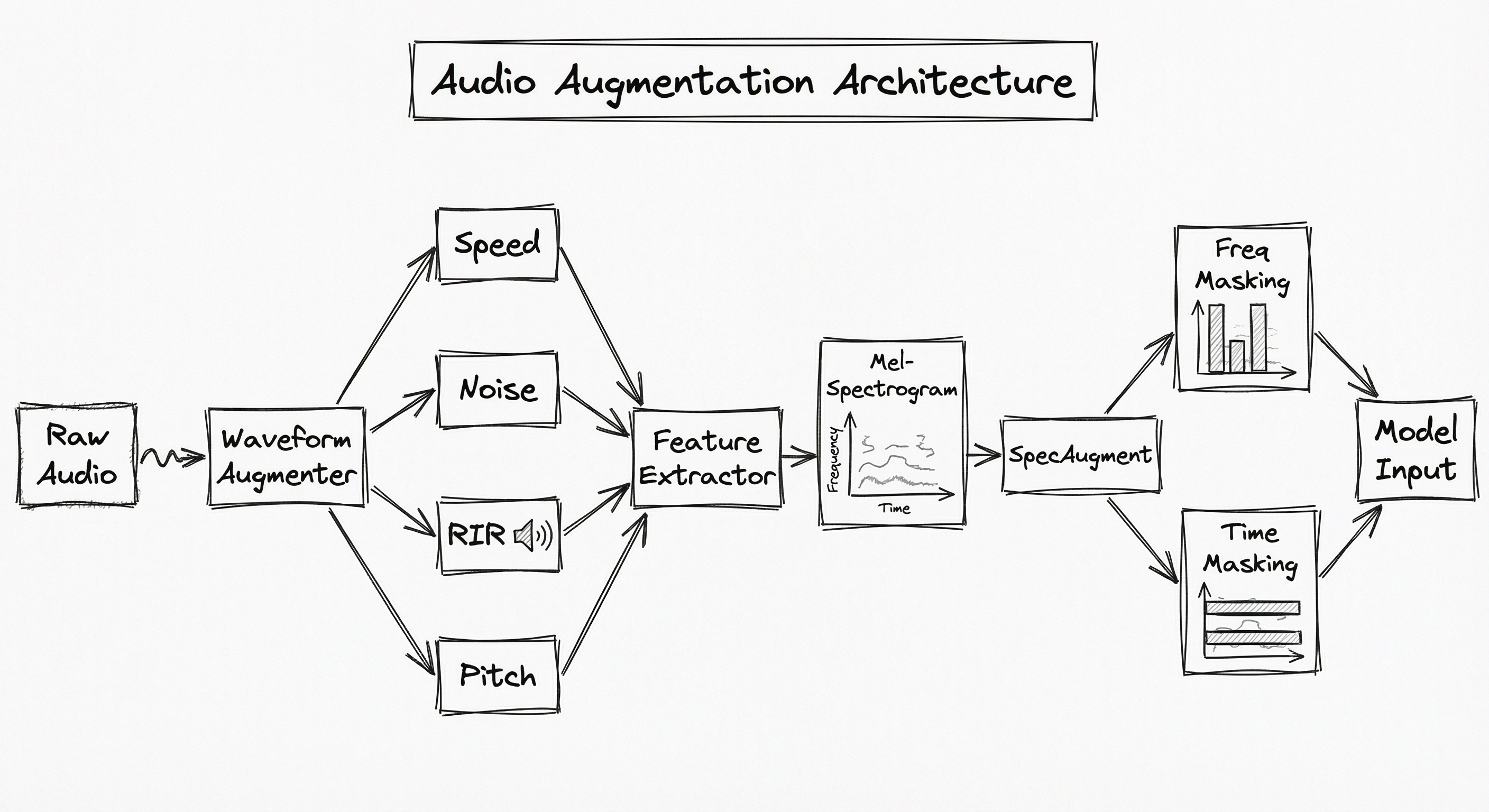
A two-stage flow: raw audio passes through a waveform augmenter (branching into speed perturbation, noise injection, RIR convolution, and pitch shift), converges at the feature extractor to produce mel-spectrograms, which then pass through SpecAugment (frequency masking and time masking) before reaching the model input.
How to Implement
Three Implementation Tiers
Tier 1: Quick start with audiomentations -- The audiomentations library provides a Compose-based API inspired by Albumentations, making it trivially easy to chain waveform augmentations. Great for prototyping and moderate-scale training. Runs on CPU.
Tier 2: GPU-accelerated with torchaudio + torch-audiomentations -- For large-scale training where CPU augmentation becomes a bottleneck, torchaudio.transforms and torch-audiomentations run augmentations directly on GPU tensors. SpecAugment is natively supported in torchaudio.
Tier 3: Full pipeline with SpeechBrain or NVIDIA NeMo -- Production ASR frameworks like SpeechBrain and NeMo include built-in augmentation pipelines with speed perturbation, noise injection, RIR convolution, and SpecAugment, all configurable via YAML. Best for teams building end-to-end ASR systems.
For most practitioners, Tier 1 is sufficient. If your GPU utilization drops below 80% during training (check with nvidia-smi), data loading is the bottleneck and you should move to Tier 2.
Cost Considerations
All augmentation libraries are open-source and free. The compute overhead is modest: waveform augmentation adds 10-20% to data loading time on CPU, and SpecAugment adds <5% on GPU. For a 1,000-hour speech dataset training run on 4x A100 GPUs, augmentation adds roughly 2-4 hours to a 48-hour training cycle -- approximately $20-40 (INR 1,700-3,400) in additional cloud GPU cost. The accuracy improvement typically far outweighs this cost.
import numpy as np
from audiomentations import (
    Compose, AddGaussianNoise, TimeStretch, PitchShift,
    Shift, Gain, AddBackgroundNoise, ApplyImpulseResponse,
    ClippingDistortion, BandPassFilter
)

# Define augmentation pipeline
transform = Compose([
    # Speed/time perturbation
    TimeStretch(min_rate=0.8, max_rate=1.2, p=0.5),
    # Pitch shift by up to 4 semitones
    PitchShift(min_semitones=-4, max_semitones=4, p=0.4),
    # Add Gaussian noise at random SNR
    AddGaussianNoise(min_amplitude=0.001, max_amplitude=0.015, p=0.5),
    # Add real-world background noise from MUSAN corpus
    AddBackgroundNoise(
        sounds_path="/data/musan/noise",
        min_snr_in_db=5.0,
        max_snr_in_db=20.0,
        p=0.5
    ),
    # Simulate room acoustics with RIR convolution
    ApplyImpulseResponse(
        ir_path="/data/openslr-28/simulated_rirs",
        p=0.3
    ),
    # Random gain adjustment
    Gain(min_gain_in_db=-6, max_gain_in_db=6, p=0.3),
    # Simulate temporal shift (circular)
    Shift(min_shift=-0.5, max_shift=0.5, p=0.3),
    # Simulate low-quality recording (clipping)
    ClippingDistortion(max_percentile_threshold=10, p=0.1),
])

# Apply to a waveform (numpy array, float32, mono)
sample_rate = 16000
audio = np.random.randn(sample_rate * 5).astype(np.float32)  # 5 seconds
augmented = transform(samples=audio, sample_rate=sample_rate)
print(f"Original shape: {audio.shape}, Augmented shape: {augmented.shape}")
The audiomentations library uses the same Compose pattern as Albumentations. Each transform has a probability p of being applied, and parameter ranges are sampled uniformly per call. Key points: (1) AddBackgroundNoise requires a directory of noise files -- the MUSAN corpus is the standard choice, freely available from openSLR. (2) ApplyImpulseResponse requires pre-recorded or simulated RIRs -- the openSLR-28 dataset provides 60,000 simulated RIRs. (3) Transforms are applied sequentially, so order matters: apply noise injection before RIR convolution to simulate noise in the reverberant room, not noise added after room simulation. (4) All transforms operate on numpy arrays at the specified sample rate.
import torch
import torchaudio
import torchaudio.transforms as T

# Load audio
waveform, sample_rate = torchaudio.load("speech.wav")

# Convert to mel-spectrogram
mel_transform = T.MelSpectrogram(
    sample_rate=16000,
    n_fft=512,
    hop_length=160,
    n_mels=80,
    f_min=20,
    f_max=8000,
)
mel_spec = mel_transform(waveform)  # (1, 80, T)

# Apply log compression
log_mel = torch.log(mel_spec + 1e-9)

# SpecAugment: frequency masking + time masking
freq_mask = T.FrequencyMasking(freq_mask_param=27)  # Max 27 frequency bands
time_mask = T.TimeMasking(time_mask_param=100)       # Max 100 time steps

# Apply two frequency masks and two time masks (standard SpecAugment policy)
augmented = log_mel
augmented = freq_mask(augmented)
augmented = freq_mask(augmented)  # Second frequency mask
augmented = time_mask(augmented)
augmented = time_mask(augmented)  # Second time mask

print(f"Original spectrogram shape: {log_mel.shape}")
print(f"Augmented spectrogram shape: {augmented.shape}")
# Shapes are identical -- SpecAugment only zeros out regions
SpecAugment operates on the spectrogram after feature extraction, not on the raw waveform. The standard SpecAugment policy (from the original Google paper) applies 2 frequency masks of width up to and 2 time masks of width up to time steps. These are applied after log-mel computation but before feeding to the model. Key advantage: SpecAugment is trivially fast (just zeroing tensor regions) and adds negligible compute overhead. It can run entirely on GPU since torchaudio.transforms are torch.nn.Module subclasses. The freq_mask_param and time_mask_param control maximum mask width -- the actual width is sampled uniformly from [0, param] each time.
import torchaudio
import torch
from torch.utils.data import Dataset, DataLoader
import random

class AugmentedSpeechDataset(Dataset):
    """ASR dataset with speed perturbation (Ko et al., 2015 method)."""

    def __init__(self, audio_paths, transcripts, speed_factors=(0.9, 1.0, 1.1)):
        # Create 3x dataset: one copy per speed factor
        self.samples = []
        for path, transcript in zip(audio_paths, transcripts):
            for speed in speed_factors:
                self.samples.append((path, transcript, speed))
        random.shuffle(self.samples)

    def __len__(self):
        return len(self.samples)

    def __getitem__(self, idx):
        path, transcript, speed = self.samples[idx]
        waveform, sample_rate = torchaudio.load(path)

        # Apply speed perturbation via resampling
        if speed != 1.0:
            # Resample: change sample rate to simulate speed change
            # e.g., speed=0.9 means slower speech, so we downsample then upsample
            new_sr = int(sample_rate * speed)
            resampler = torchaudio.transforms.Resample(
                orig_freq=sample_rate, new_freq=new_sr
            )
            waveform = resampler(waveform)
            # Resample back to original rate to keep consistent sample rate
            resampler_back = torchaudio.transforms.Resample(
                orig_freq=new_sr, new_freq=sample_rate
            )
            waveform = resampler_back(waveform)

        return waveform, transcript, sample_rate

# Usage
paths = ["utt001.wav", "utt002.wav", "utt003.wav"]
transcripts = ["hello world", "good morning", "how are you"]
dataset = AugmentedSpeechDataset(paths, transcripts)
print(f"Original size: {len(paths)}, Augmented size: {len(dataset)}")
# Output: Original size: 3, Augmented size: 9 (3x expansion)
Speed perturbation is the simplest and most widely used audio augmentation for ASR, introduced by Ko et al. (2015). It creates 3 copies of each utterance at speeds 0.9x, 1.0x, and 1.1x, effectively tripling the dataset. Unlike time stretching (which preserves pitch), speed perturbation changes both tempo and pitch simultaneously -- this is desirable for ASR because it simulates natural speaker variability (slower speakers tend to have lower pitch). This is the standard Kaldi recipe, used in virtually every competitive ASR system. The 0.9/1.0/1.1 factors were empirically validated across multiple benchmarks, yielding an average relative WER improvement of 4.3%.
import torch
import torchaudio
import torchaudio.transforms as T
from audiomentations import Compose, AddGaussianNoise, AddBackgroundNoise, Gain
import numpy as np

class AudioAugmentationPipeline:
    """Combined waveform + spectrogram augmentation for ASR training."""

    def __init__(self, musan_path, rir_path, sample_rate=16000):
        self.sample_rate = sample_rate

        # Stage 1: Waveform augmentation (CPU, numpy)
        self.waveform_aug = Compose([
            AddGaussianNoise(min_amplitude=0.001, max_amplitude=0.01, p=0.3),
            AddBackgroundNoise(
                sounds_path=musan_path,
                min_snr_in_db=5, max_snr_in_db=20, p=0.5
            ),
            Gain(min_gain_in_db=-6, max_gain_in_db=6, p=0.3),
        ])

        # Stage 2: Feature extraction (GPU, torch)
        self.mel_spec = T.MelSpectrogram(
            sample_rate=sample_rate,
            n_fft=512, hop_length=160, n_mels=80
        )

        # Stage 3: SpecAugment (GPU, torch)
        self.freq_mask = T.FrequencyMasking(freq_mask_param=27)
        self.time_mask = T.TimeMasking(time_mask_param=100)

    def __call__(self, waveform_np, is_training=True):
        # Stage 1: Waveform augmentation (only during training)
        if is_training:
            waveform_np = self.waveform_aug(
                samples=waveform_np, sample_rate=self.sample_rate
            )

        # Convert to torch tensor
        waveform = torch.from_numpy(waveform_np).unsqueeze(0)  # (1, T)

        # Stage 2: Extract mel-spectrogram
        mel = self.mel_spec(waveform)
        log_mel = torch.log(mel + 1e-9)

        # Stage 3: SpecAugment (only during training)
        if is_training:
            log_mel = self.freq_mask(log_mel)
            log_mel = self.freq_mask(log_mel)  # 2x freq masks
            log_mel = self.time_mask(log_mel)
            log_mel = self.time_mask(log_mel)   # 2x time masks

        return log_mel

# Usage
pipeline = AudioAugmentationPipeline(
    musan_path="/data/musan/noise",
    rir_path="/data/openslr-28",
)
audio = np.random.randn(16000 * 3).astype(np.float32)  # 3 seconds
features = pipeline(audio, is_training=True)
print(f"Output features shape: {features.shape}")
This shows the recommended production pattern: a two-stage pipeline that combines waveform augmentation (using audiomentations on CPU/numpy) with spectrogram augmentation (using torchaudio on GPU/torch). The pipeline is callable and accepts a training flag to disable augmentation during validation/inference. Key design decisions: (1) Waveform augmentation runs on CPU during data loading, leveraging multi-worker DataLoader parallelism. (2) Feature extraction and SpecAugment run on GPU for speed. (3) The is_training flag ensures validation and test data are not augmented, maintaining evaluation consistency. This pattern is used in production ASR systems at scale.
# Audio augmentation config (YAML) for ASR training pipeline
augmentation:
  waveform:
    speed_perturbation:
      factors: [0.9, 1.0, 1.1]
      mode: "expand_dataset"  # Create 3 copies per utterance
    noise_injection:
      noise_corpus: "/data/musan/noise"
      snr_range_db: [5, 20]
      probability: 0.5
    rir_convolution:
      rir_corpus: "/data/openslr-28/simulated_rirs"
      probability: 0.3
    pitch_shift:
      semitones_range: [-3, 3]
      probability: 0.3
    gain:
      range_db: [-6, 6]
      probability: 0.3
  spectrogram:
    specaugment:
      freq_mask_param: 27
      time_mask_param: 100
      num_freq_masks: 2
      num_time_masks: 2
  feature_extraction:
    type: "mel_spectrogram"
    sample_rate: 16000
    n_fft: 512
    hop_length: 160
    n_mels: 80
    f_min: 20
    f_max: 8000
Common Implementation Mistakes
- ●
Applying augmentation after feature extraction when it should be before: Noise injection and RIR convolution operate on waveforms, not spectrograms. Adding Gaussian noise to a mel-spectrogram is not equivalent to adding acoustic noise to the waveform -- the spectral characteristics will be wrong. Always apply time-domain augmentations before feature extraction, and only use SpecAugment-family transforms on spectrograms.
- ●
Using mismatched sample rates: If your model expects 16 kHz audio but your noise corpus is at 44.1 kHz, mixing them without resampling introduces frequency aliasing artifacts. Always resample noise files, RIRs, and background audio to match the target sample rate before mixing.
- ●
Over-augmenting short utterances: A 0.5-second utterance augmented with aggressive time masking (SpecAugment T=100 frames) might have most of its content masked, leaving the model with almost no useful signal. Scale masking parameters relative to utterance length: use
time_mask_param = min(T_max, int(0.05 * utterance_frames)). - ●
Ignoring the effect of speed perturbation on transcription alignment: Speed perturbation changes audio duration. If you are training a CTC or attention-based ASR model with forced alignment, the alignment labels must be adjusted accordingly. Failing to do so causes the model to learn incorrect alignments, degrading performance.
- ●
Applying pitch shifting beyond natural speaker range: Shifting pitch by more than 4-5 semitones produces unnatural-sounding audio that does not resemble any real speaker. The model may learn to handle these unrealistic variations at the expense of performance on natural speech. Keep pitch shift within +/- 4 semitones for speech tasks.
- ●
Not normalizing after augmentation: Noise injection and gain adjustment can push waveform amplitude outside the [-1, 1] range, causing clipping. Always apply peak normalization or RMS normalization after the augmentation chain to prevent clipping artifacts.
When Should You Use This?
Use When
You have limited labeled audio data (<1,000 hours for ASR, <10,000 samples for classification) and need to prevent overfitting without expensive data collection
Your training audio was recorded in controlled conditions (studio, quiet room) but the model will deploy in noisy, reverberant, or variable acoustic environments
You are building a speech recognition system for low-resource languages (e.g., Indian languages like Odia, Assamese, Maithili) where labeled data is scarce
You need robustness to speaker variability -- different speaking speeds, pitch ranges, and vocal characteristics -- without collecting audio from thousands of speakers
Your model will encounter diverse recording devices -- from studio microphones to budget smartphone mics to far-field smart speakers -- each with different frequency responses
You are training a sound event detection or environmental sound classification model where real-world acoustic conditions are highly variable
You are fine-tuning a pre-trained model (Whisper, Wav2Vec 2.0) on a domain-specific dataset and need to prevent catastrophic forgetting while improving domain robustness
Avoid When
Your training data already covers the full range of deployment conditions -- e.g., you have 100,000+ hours of naturally noisy, diverse audio with matched transcriptions. At this scale, augmentation provides diminishing returns and slows training
The augmentation would violate label semantics -- e.g., pitch-shifting a musical instrument recognition dataset where pitch is the label, or time-stretching a tempo detection task where duration is the target
You are training a speaker verification or speaker identification model and pitch shifting would change the speaker's vocal identity, confusing the model about who is speaking
Inference latency is critical and you cannot afford test-time augmentation overhead -- e.g., real-time ASR on edge devices where even the standard pipeline runs at the latency limit
You are working with pre-processed features (embeddings from a frozen encoder) where the augmentation needs to happen before the encoder, not after. In this case, augmentation must be part of the encoder's training, not your downstream task
Your audio task is inherently clean-room -- e.g., medical ultrasound signal analysis or industrial vibration monitoring where noise and room acoustics are controlled and consistent
Key Tradeoffs
The Core Tradeoff: Robustness vs Training Cost
Audio augmentation trades compute time for data diversity. A 1,000-hour ASR dataset with speed perturbation (3x) + noise injection + RIR convolution + SpecAugment effectively becomes a 3,000-hour dataset with per-epoch variation. This typically adds 15-25% to training time:
| Pipeline | Training Time (per epoch, 4x A100) | Estimated Cost |
|---|---|---|
| No augmentation | ~2 hours | ~$15 (INR 1,250) |
| Speed perturbation only | ~6 hours (3x data) | ~$45 (INR 3,750) |
| Speed + noise + SpecAugment | ~7 hours | ~$52 (INR 4,350) |
| Full pipeline (all augmentations) | ~8 hours | ~$60 (INR 5,000) |
But you typically need fewer epochs to converge (the augmented model generalizes faster), so total training cost often stays comparable. And the WER improvement of 10-30% relative easily justifies the marginal cost increase.
The Augmentation Ordering Tradeoff
The order in which augmentations are applied matters and encodes assumptions about the acoustic environment:
- Noise before RIR: Simulates noise sources in the same room as the speaker (the noise also reverberates). More realistic for indoor scenarios.
- RIR before noise: Simulates noise added at the microphone after room effects (e.g., electronic noise, or noise in a different acoustic space). More realistic for recording device noise.
For general-purpose ASR, noise-before-RIR is the standard choice, but the optimal order depends on your deployment environment.
The SpecAugment Strength Tradeoff
Stronger SpecAugment (larger mask widths, more masks) provides more regularization but can destroy too much information in short utterances. The original paper used (frequency mask) and (time mask) for LibriSpeech, but these values may need reduction for:
- Short utterances (<2 seconds): Reduce to avoid masking >50% of the spectrogram
- Narrow-band audio (telephone, 8 kHz): Reduce proportionally to the narrower frequency range
- Small models: Weaker regularization may be needed to prevent underfitting
Rule of Thumb: Start with speed perturbation (0.9/1.0/1.1) + SpecAugment (standard policy). This is the minimum viable augmentation for any speech task. Add noise injection and RIR convolution only if your deployment environment is noisy or reverberant. Pitch shifting is most useful for speaker-diverse applications.
Alternatives & Comparisons
Image augmentation applies spatial and photometric transforms to images, while audio augmentation applies temporal and spectral transforms to audio signals. Both share the same goal (data diversity without new labels) and similar principles (label-preserving transforms, on-the-fly application). Audio augmentation is more domain-specific: techniques like RIR convolution and SpecAugment have no direct image analogues, while image techniques like rotation and flipping have no direct audio analogues. If your task involves spectrograms treated as images (e.g., environmental sound classification), you might use image augmentation techniques on spectrograms as a complement to audio-specific transforms.
Text augmentation modifies discrete token sequences (synonym replacement, back-translation, paraphrasing), while audio augmentation manipulates continuous signals. Text augmentation is harder because small word changes can flip semantic meaning, while audio augmentation is more forgiving -- adding noise or shifting pitch rarely changes what is being said. For end-to-end speech-to-text systems, audio augmentation is generally more impactful than text-side augmentation, but some systems use both: augmenting audio inputs and augmenting text targets (e.g., for language model training).
GANs (WaveGAN, MelGAN, HiFi-GAN) generate entirely new audio samples rather than transforming existing ones. This is more powerful for creating novel speaker voices or acoustic conditions not present in training data, but requires training a generative model (expensive: days of GPU time, INR 50,000-2 lakh in compute). Audio augmentation is a lightweight alternative: zero model training required, near-instant application, and guaranteed label preservation. Use GANs when you need to synthesize new audio categories or voices; use augmentation when you need diversity within existing categories.
Pros, Cons & Tradeoffs
Advantages
Dramatically improves noise robustness with near-zero marginal cost -- adding MUSAN noise at random SNRs during training can reduce WER by 20-40% relative in noisy conditions, at the cost of a few extra CPU cycles per batch.
SpecAugment is arguably the highest-ROI technique in speech ML -- it requires zero additional data, zero architectural changes, and zero hyperparameter search, yet consistently delivers 10-30% relative WER improvement across ASR benchmarks.
Speed perturbation is trivially simple and universally effective -- creating 3 copies of the dataset at speeds 0.9x/1.0x/1.1x yields a consistent 3-5% relative improvement and has become the de facto standard in every competitive ASR recipe.
Simulates real-world deployment conditions synthetically -- RIR convolution, background noise, and gain variation allow you to train for reverberant rooms, noisy streets, and variable recording devices without physically collecting audio in those environments.
Mature, production-ready open-source libraries (
audiomentations,torchaudio,torch-audiomentations, SpeechBrain, NeMo) provide battle-tested implementations with active maintenance and extensive documentation.Combines naturally with other regularization techniques -- augmentation is orthogonal to dropout, weight decay, and label smoothing. Using all of them together typically yields the best results.
Critical enabler for low-resource languages -- for Indian languages (and other languages with <100 hours of labeled data), augmentation is often the difference between a usable model and a non-functional one, stretching limited data to achieve production-quality recognition.
Disadvantages
Increases training time by 15-40% depending on the augmentation chain complexity. For very large datasets (>100,000 hours), this overhead can translate to thousands of dollars (lakhs of INR) in additional GPU costs with diminishing accuracy returns.
Incorrect augmentation can degrade performance -- pitch-shifting a speaker ID system, time-stretching a tempo detection model, or over-masking short utterances with SpecAugment all violate label semantics and silently hurt accuracy.
Requires domain expertise to design augmentation policies -- the right augmentation for ASR (speed perturbation, noise, RIR) is different from music classification (time stretch, pitch shift, no RIR) and environmental sound detection (noise mixup, no speed perturbation). No universal policy works for all audio tasks.
Noise corpus and RIR dataset management adds infrastructure complexity -- you need to source, store, and serve potentially gigabytes of noise files and RIR recordings. The MUSAN corpus alone is 11 GB, and comprehensive RIR sets can be 50+ GB.
CPU bottleneck at scale -- waveform augmentations (especially time stretching and pitch shifting via phase vocoder) are CPU-intensive. For large batch sizes on multi-GPU setups, augmentation in the data loader can become the training bottleneck if not properly parallelized.
Test-time augmentation (TTA) is rarely practical for audio -- unlike vision where TTA is common, audio TTA requires generating and processing multiple time-stretched/noise-injected variants, each potentially seconds or minutes long, making it too slow for real-time speech applications.
Failure Modes & Debugging
Label-violating augmentation for pitch/tempo-sensitive tasks
Cause
Applying pitch shifting to a musical key detection model, speed perturbation to a tempo estimation model, or time stretching to a duration-based phonetic classification task. In these cases, the augmentation directly modifies the feature that the label depends on.
Symptoms
Validation accuracy drops below the no-augmentation baseline. The model produces inconsistent predictions for the same audio at different augmentation strengths. Training loss converges normally but validation metrics worsen, indicating the model is learning corrupted label-feature relationships.
Mitigation
Map out which audio properties your labels depend on and exclude augmentations that modify those properties. For musical pitch tasks, avoid pitch shifting. For tempo tasks, avoid speed perturbation and time stretching. For speaker ID, be cautious with pitch shifting (it changes perceived speaker identity). Create a label sensitivity matrix that documents which augmentations are safe for each task in your pipeline.
Over-aggressive SpecAugment on short utterances
Cause
Using SpecAugment parameters calibrated for long utterances (e.g., frames) on short commands or keywords that span only 50-100 frames total. A single time mask can obliterate 50-100% of the useful signal, leaving the model with essentially no input to learn from.
Symptoms
Training loss on short utterances stays high while long utterances converge normally. The model systematically misrecognizes short commands ("yes", "no", "stop") but handles longer sentences well. If you log per-utterance loss, short utterances show much higher variance.
Mitigation
Scale SpecAugment parameters relative to utterance length. Use adaptive masking: time_mask_param = min(T_max, int(p_ratio * num_frames)) where p_ratio is the maximum fraction of frames to mask (typically 0.05-0.10). Alternatively, use the p parameter in torchaudio.transforms.TimeMasking to limit the mask width as a proportion of the spectrogram length. Monitor per-length-bucket metrics during training to detect this failure early.
Noise-augmented model fails on clean audio
Cause
Training exclusively with heavy noise augmentation (low SNR, high probability) without including clean audio in the training mix. The model learns to expect noise and performs poorly on noise-free inputs -- it may even hallucinate words from the expected noise pattern.
Symptoms
The model performs well in noisy conditions but degrades on clean, studio-quality audio. WER on clean test sets is higher than expected. The model occasionally inserts spurious words or phonemes that correspond to noise patterns it learned to decode.
Mitigation
Always include the original unaugmented audio in the training mix alongside augmented variants. Speed perturbation naturally handles this (1.0x factor = unaugmented). For noise injection, ensure the original clean version is seen at least once per epoch. Use a balanced augmentation schedule where 30-50% of samples are unaugmented. This ensures the model handles both clean and noisy conditions.
Sample rate mismatch between noise corpus and target audio
Cause
Mixing noise files recorded at 44.1 kHz or 48 kHz into target audio at 16 kHz without proper resampling. The noise signal is decimated without anti-aliasing, introducing frequency aliasing artifacts that create unnatural high-frequency content. The model learns to handle these artifacts rather than real-world noise.
Symptoms
The model's noise robustness does not transfer to real-world noisy audio despite good validation metrics on augmented data. Spectrograms of augmented audio show unusual high-frequency energy patterns not present in real noisy recordings. The model may develop sensitivity to aliasing frequencies that are absent in deployment.
Mitigation
Pre-process all noise corpora and RIR files to match the target sample rate before training begins. Use high-quality resampling (e.g., torchaudio.transforms.Resample with rolloff=0.99 or librosa.resample with res_type='kaiser_best'). Verify by visual inspection of spectrograms: augmented audio spectrograms should look similar to naturally noisy recordings at the same SNR.
Augmentation pipeline CPU bottleneck starving GPUs
Cause
Complex waveform augmentation chains (time stretching + pitch shifting + RIR convolution + noise injection) running on a single CPU core in the data loader, while multiple GPUs wait idle for the next batch. The phase vocoder algorithm used for time stretching is particularly CPU-intensive.
Symptoms
GPU utilization drops below 70% during training (visible via nvidia-smi). Training throughput (utterances/second) does not scale linearly with the number of GPUs. Profiling shows the data loading step takes 3-10x longer than the model forward+backward pass.
Mitigation
Use num_workers=4-8 in PyTorch DataLoader to parallelize augmentation across CPU cores. Replace CPU-bound transforms with GPU equivalents: use torch-audiomentations (GPU-native) instead of audiomentations (CPU-only) for the heaviest transforms. Pre-compute speed-perturbed versions offline (they are deterministic) and apply stochastic augmentations on-the-fly. For extreme scale, use NVIDIA DALI for GPU-accelerated data loading and augmentation.
Placement in an ML System
Where Does It Sit in the Pipeline?
Audio augmentation occupies two positions in the ML pipeline:
Position 1: Waveform stage (after audio decoding, before feature extraction). This is where time-domain augmentations live: speed perturbation, noise injection, RIR convolution, pitch shifting, gain adjustment. These must happen on the raw waveform because they simulate physical acoustic phenomena that affect the signal before it reaches any analysis stage.
Position 2: Feature stage (after feature extraction, before model input). This is where SpecAugment lives: frequency masking and time masking on the mel-spectrogram. These are purely computational regularizers with no physical analogue.
The typical pipeline flow:
- Audio Loading: Read WAV/FLAC from disk, decode to float32 tensor
- Resampling: Convert to target sample rate (e.g., 16 kHz for speech)
- Waveform Augmentation: Speed perturbation, noise injection, RIR, pitch shift
- Peak Normalization: Clip and normalize to [-1, 1] range
- Feature Extraction: Compute mel-spectrogram (80 bands, 25ms window, 10ms hop)
- SpecAugment: Apply frequency and time masking
- Batch Collation: Pad/truncate to uniform length, stack into batch tensor
- Model Input: Feed to encoder (Conformer, Transformer, CNN)
Critical Placement Notes
Waveform augmentations must happen before feature extraction. Adding noise to a mel-spectrogram is not equivalent to adding noise to the waveform -- the spectral distribution will be wrong (mel-spectrogram noise would be uniform in log-mel space, while real noise is typically concentrated in specific frequency bands).
SpecAugment must happen after feature extraction. It operates on the spectrogram tensor and has no meaning in the waveform domain.
Speed perturbation is unique: it can be applied either on-the-fly (random factor per epoch) or as a dataset expansion (pre-generate 3 copies at fixed factors). The latter is more common because it is deterministic and simplifies training logistics.
Key Insight: Audio augmentation is the acoustic immune system of your model. Just as the immune system learns to fight infections by exposure to weakened pathogens, the model learns to handle noisy, reverberant, variable-speed audio by training on augmented versions. The waveform stage simulates real pathogens (physical acoustic conditions), while SpecAugment is more like a general fitness routine (input regularization). Both are essential for a healthy, robust model.
Pipeline Stage
Data Preprocessing / Training Pipeline
Upstream
- audio-decoder
- data-loader
- feature-extraction
Downstream
- mel-spectrogram
- model-training
- speech-to-text
Scaling Bottlenecks
The primary bottleneck is CPU throughput for waveform-level augmentation. Time stretching (phase vocoder) and pitch shifting are computationally expensive: processing a single 10-second utterance takes 5-15ms per transform. Chaining 4-5 transforms per utterance at scale (1,000+ hours, batch size 64, 8 GPUs) can saturate CPU cores.
Quantitative impact: On a typical training node (64 CPU cores, 8x A100 GPUs), waveform augmentation with a full pipeline (speed perturbation + noise + RIR + pitch shift) processes about 2,000-4,000 utterances/second. If your model consumes batches faster than this, GPUs will idle.
Solutions by cost:
- Multi-worker DataLoader (free): Set
num_workers=8-16to parallelize across CPU cores. Linear speedup up to ~16 workers. - Pre-compute deterministic augmentations (free): Speed perturbation with fixed factors (0.9, 1.0, 1.1) can be pre-computed once and saved to disk. Only apply stochastic augmentations on-the-fly.
- torch-audiomentations on GPU ($0 software, uses GPU memory): Move waveform augmentation to GPU, freeing CPU for data loading.
- NVIDIA DALI ($0 software, requires NVIDIA GPUs): End-to-end GPU-accelerated data pipeline from audio decoding through augmentation to feature extraction.
- Distributed data loading (infrastructure cost): For multi-node training, use WebDataset or FFCV to distribute augmented data loading across machines.
SpecAugment on spectrograms is never a bottleneck -- it is a simple tensor masking operation that runs in microseconds on GPU.
Production Case Studies
Google Brain developed SpecAugment, a deceptively simple augmentation method that applies time warping, frequency masking, and time masking directly to mel-spectrograms during ASR training. The technique requires no additional data, no external noise corpora, and no changes to the model architecture. SpecAugment was applied to Listen, Attend and Spell (LAS) models trained on LibriSpeech 960h. The standard SpecAugment policy uses 2 frequency masks of width up to 27 bands and 2 time masks of width up to 100 frames. Combined with a language model, SpecAugment achieved 5.8% WER on LibriSpeech test-other, pushing past previous state-of-the-art results. A follow-up paper (SpecAugment on Large Scale Datasets) confirmed that the technique scales to larger datasets and models, maintaining consistent relative improvements.
SpecAugment reduced WER on LibriSpeech test-other from 12.5% to 6.8% without a language model (46% relative improvement), and to 5.8% with shallow fusion. The technique became the de facto standard for ASR training and is now included in every major speech toolkit (torchaudio, SpeechBrain, NeMo, ESPnet). Its simplicity and effectiveness made it one of the most cited papers in speech processing.
Sarvam AI, an Indian startup backed by Peak XV Partners, built Sarvam Audio, a speech recognition system supporting 10+ Indian languages (Hindi, Tamil, Telugu, Kannada, Bengali, Marathi, and others). Training robust ASR for Indian languages is uniquely challenging: limited labeled data per language (often <500 hours), extreme acoustic diversity (noisy streets, crowded homes, reverberant temples, low-quality smartphone microphones), and code-switching between languages. Sarvam uses extensive audio augmentation including speed perturbation (0.9x/1.0x/1.1x), noise injection with Indian ambient sounds (traffic, market noise, festival sounds), RIR convolution to simulate diverse room acoustics, and SpecAugment for regularization. Their pre-training on 2 trillion tokens of Indic data, combined with augmented audio fine-tuning, produced a model that handles conversational, multi-speaker, and long-duration audio across Indian languages.
Sarvam Audio achieves competitive WER across 10 Indian languages, with particular strength in noisy and conversational settings where standard models (like Whisper) struggle with code-switching and Indian accents. The system serves production traffic through Sarvam's API platform, processing voice interactions for Indian enterprise customers. Audio augmentation was cited as a critical factor in achieving robustness across India's diverse acoustic environments.
Meta's FAIR lab developed WavAugment, a time-domain augmentation library, and demonstrated its impact on self-supervised speech representation learning via Contrastive Predictive Coding (CPC). The key insight: augmentation is even more critical for self-supervised learning than supervised learning, because the model must learn robust representations without labels. WavAugment applies pitch modification (up to +/- 300 cents), additive noise (MUSAN corpus at 5-15 dB SNR), reverberation (RIR convolution), and their combinations to the raw waveform during CPC pre-training. The study systematically evaluated each augmentation type and their combinations, finding that the full combination provided the largest gains.
A combination of pitch modification, additive noise, and reverberation improved CPC representations by 18-22% relative on downstream phone classification and speaker identification tasks. Critically, the augmented CPC model trained on just 600 hours of LibriSpeech data matched the performance of the Libri-light model trained on 60,000 hours -- a 100x data efficiency improvement. WavAugment is open-sourced and has been adopted by several self-supervised speech research groups.
Vakyansh is an open-source end-to-end ASR toolkit developed under India's Digital Public Infrastructure initiative, targeting 18 low-resource Indic languages. The project faced severe data scarcity: some languages had fewer than 100 hours of transcribed speech. To overcome this, Vakyansh built automated data creation pipelines that crawl, segment, and label speech from public sources (YouTube, All India Radio, Lok Sabha TV), then applied aggressive audio augmentation including 3-way speed perturbation, multi-condition noise injection (Indian environmental sounds: auto-rickshaw traffic, market vendors, railway station announcements, monsoon rain), and SpecAugment. The augmentation pipeline was designed specifically for Indian acoustic conditions, with noise samples collected from Indian cities and RIRs measured in typical Indian building types (concrete apartments, temple halls, government offices).
Vakyansh produced state-of-the-art ASR models for 18 Indic languages, with 14,000 hours of speech data created through automated pipelines. Audio augmentation was identified as the single most impactful technique for low-resource languages, providing 15-25% relative WER improvement across languages. The models are open-sourced and deployed in Indian government digital services.
Tooling & Ecosystem
The most popular Python library for waveform-level audio augmentation, inspired by Albumentations (image augmentation). Provides 30+ transforms including AddGaussianNoise, TimeStretch, PitchShift, AddBackgroundNoise, ApplyImpulseResponse, Gain, ClippingDistortion, BandPassFilter, and more. Uses a Compose API with per-transform probability control. Operates on numpy arrays. Has helped users achieve top results in Kaggle audio competitions. Version 0.43+ as of 2026.
PyTorch's official audio processing library with built-in SpecAugment implementations (FrequencyMasking, TimeMasking, TimeStretch), plus MelSpectrogram, MFCC, and other feature extractors. All transforms are torch.nn.Module subclasses, enabling GPU execution and integration with torch.nn.Sequential. The go-to choice for SpecAugment in PyTorch pipelines.
GPU-accelerated audio augmentation library that operates directly on PyTorch tensors, avoiding the CPU-GPU data transfer bottleneck of audiomentations (which uses numpy). Supports batched augmentation on GPU, making it ideal for large-scale training. Provides AddBackgroundNoise, ApplyImpulseResponse, Gain, PeakNormalization, and more. Best for multi-GPU setups where CPU augmentation becomes the bottleneck.
An all-in-one PyTorch-based speech toolkit that includes built-in augmentation pipelines for ASR, speaker verification, speech enhancement, and more. Augmentation is configured via YAML recipes and supports speed perturbation, noise injection, reverberation, SpecAugment, and custom transforms. Includes pre-built recipes for LibriSpeech, CommonVoice, and other benchmarks with augmentation enabled by default.
NVIDIA's conversational AI toolkit with production-grade augmentation pipelines for ASR. Supports speed perturbation, SpecAugment, noise perturbation, and impulse response augmentation via YAML config. Optimized for multi-GPU training on NVIDIA hardware with DALI integration for GPU-accelerated data loading. Used in production by enterprises for building custom ASR systems.
Meta's time-domain audio augmentation library built on libsox, providing ~50 audio effects including reverb, pitch, speed, tempo, and more. Designed for speech representation learning research. Allows interleaving libsox and PyTorch-based effects. Particularly effective for self-supervised pre-training pipelines (CPC, wav2vec). Lightweight and easy to integrate.
A Python library for room acoustics simulation and Room Impulse Response (RIR) generation. Simulates rooms of arbitrary geometry with configurable wall materials, microphone arrays, and sound sources. Generates synthetic RIRs for augmentation without requiring real room recordings. Essential for teams that need diverse room acoustics but lack access to measured RIR databases.
Research & References
Park, D.S., Chan, W., Zhang, Y., Chiu, C.C., Zoph, B., Cubuk, E.D., Le, Q.V. (2019)Interspeech 2019
Introduced SpecAugment, which applies time warping, frequency masking, and time masking directly to mel-spectrograms during ASR training. Achieved state-of-the-art on LibriSpeech (6.8% WER on test-other without LM) and Switchboard (6.8% WER) with zero architectural changes. Became the single most impactful augmentation technique in modern ASR.
Ko, T., Peddinti, V., Povey, D., Khudanpur, S. (2015)Interspeech 2015
Proposed speed perturbation as a simple audio augmentation strategy: create 3 copies of training data at speed factors 0.9, 1.0, and 1.1. Evaluated on 4 LVCSR tasks (100-960 hours), achieving 4.3% average relative WER improvement. Established speed perturbation as the standard baseline augmentation for ASR. The method has near-zero implementation cost and remains ubiquitous in Kaldi and modern ASR recipes.
Kharitonov, E., Riviere, M., Synnaeve, G., Wolf, L., Mazare, P.E., Douze, M., Dupoux, E. (2021)SLT 2020 (IEEE Spoken Language Technology Workshop)
Systematically studied the effect of time-domain augmentation (pitch modification, additive noise, reverberation) on self-supervised speech learning via CPC. Found that combined augmentation improves downstream performance by 18-22% relative and achieves results comparable to 100x more training data. Released the WavAugment library.
Meng, L., Xu, J., Tan, X., Wang, J., Qin, T., Xu, B. (2021)ICASSP 2021
Applied the Mixup principle to speech: mix spectrograms of two utterances with interpolation coefficient , and train the model to recognize both transcriptions with loss weighted by . Achieved 10.6% relative PER improvement on TIMIT and 4.7% WER on WSJ, outperforming SpecAugment alone. Demonstrated that audio mixing is effective for low-resource ASR.
Snyder, D., Chen, G., Povey, D. (2015)arXiv preprint
Introduced MUSAN, a free corpus containing over 900 noises, 42 hours of music, and 60 hours of speech in 12 languages, released under Creative Commons license. Became the standard noise corpus for audio augmentation in speech processing. Used for voice activity detection training, speaker verification augmentation, and ASR noise robustness. Available from openSLR.
Ravanelli, M., Parcollet, T., Plantinga, P., et al. (2021)arXiv preprint (JMLR 2024 for v1.0)
Presented SpeechBrain, an open-source PyTorch toolkit for speech processing with built-in augmentation support. Includes on-the-fly waveform augmentation (noise, reverberation, speed perturbation) and SpecAugment, all configurable via YAML recipes. Provides pre-built recipes for ASR, speaker verification, speech enhancement, and separation. Adopted by hundreds of research groups and deployed in production systems.
Interview & Evaluation Perspective
Common Interview Questions
- ●
What is audio augmentation and why is it important for speech recognition systems?
- ●
Explain SpecAugment. What does it do, and why is masking parts of the spectrogram helpful?
- ●
What is the difference between speed perturbation and time stretching? When would you use each?
- ●
How does noise injection work in audio augmentation? What parameters are important?
- ●
Explain Room Impulse Response (RIR) convolution. How does it simulate real room acoustics?
- ●
You are building an ASR system for Indian languages with limited training data. What augmentation strategy would you design?
- ●
Your ASR model works well on clean audio but fails in noisy environments. How would you diagnose and fix this?
- ●
What is the difference between waveform-domain and spectrogram-domain augmentation? Give examples of each.
- ●
How would you handle audio augmentation in a real-time, low-latency speech recognition pipeline?
- ●
Compare audio augmentation with collecting more diverse training data. When is each approach preferable?
Key Points to Mention
- ●
Audio augmentation operates in two complementary domains: time-domain (waveform manipulation: noise injection, speed perturbation, pitch shifting, RIR convolution) and frequency-domain (spectrogram manipulation: SpecAugment frequency/time masking). Production pipelines use both.
- ●
SpecAugment is the single highest-ROI technique: zero additional data, zero model changes, 10-30% relative WER improvement. Standard policy: 2 frequency masks (F=27), 2 time masks (T=100).
- ●
Speed perturbation (0.9x, 1.0x, 1.1x) is the simplest and most universal augmentation. It changes both tempo and pitch, simulating speaker variability. Triples dataset size with 4.3% average relative WER improvement.
- ●
Noise injection uses a noise corpus (MUSAN is the standard) mixed at random SNR (5-20 dB). The SNR range should match expected deployment conditions. Always include clean (unaugmented) samples to avoid degrading performance on clean audio.
- ●
RIR convolution simulates room acoustics by convolving the signal with a measured or synthetic impulse response. This is critical for far-field ASR (smart speakers, conference systems) where reverberation significantly degrades recognition.
- ●
For low-resource Indian languages, augmentation is essential: speed perturbation + noise injection with Indian ambient sounds + SpecAugment can provide 15-25% relative WER improvement when data is scarce.
- ●
The augmentation pipeline must respect label semantics: do not pitch-shift for pitch-dependent tasks, do not time-stretch for tempo-dependent tasks, do not over-mask short utterances with SpecAugment.
- ●
CPU bottleneck is the main scalability concern. Solutions: multi-worker DataLoader, GPU augmentation (torch-audiomentations), pre-compute deterministic augmentations (speed perturbation), or NVIDIA DALI.
Pitfalls to Avoid
- ●
Failing to distinguish between waveform-domain and spectrogram-domain augmentation -- they serve different purposes and are applied at different pipeline stages. Conflating them suggests shallow understanding.
- ●
Suggesting that augmentation can replace diverse data collection. Augmentation creates variations within the existing data distribution, not new data points. If your dataset has no female speakers, augmentation cannot create female speech.
- ●
Not mentioning SpecAugment when discussing audio augmentation. As of 2026, SpecAugment is the most universally applied audio augmentation technique and omitting it is a significant gap.
- ●
Applying audio augmentation techniques designed for speech (speed perturbation, noise injection) to non-speech audio tasks (music classification, environmental sound detection) without considering whether they preserve labels in that domain.
- ●
Ignoring the compute cost dimension. Senior interviewers want to hear about tradeoffs: augmentation adds 15-40% training overhead, requires noise corpus management, and can bottleneck CPU. Quantify the costs alongside the benefits.
Senior-Level Expectation
A senior/staff candidate should discuss the full augmentation architecture: two-stage pipeline (waveform + spectrogram), augmentation policy design (which transforms, probabilities, parameter ranges), noise corpus management (sourcing, storing, and serving MUSAN, RIRs), and compute optimization (multi-worker DataLoader, GPU augmentation, pre-computation). They should articulate domain-specific augmentation design: speech tasks need speed perturbation + noise + RIR + SpecAugment, music tasks need independent time stretch + pitch shift, environmental sound tasks need background mixing. They should quantify tradeoffs: 15-40% training overhead for 10-30% WER improvement, the cost of noise corpora (MUSAN 11 GB, RIR sets 50+ GB), and the point of diminishing returns. For Indian language ASR specifically, they should discuss the unique challenges (code-switching, diverse acoustic environments, scarcity of labeled data) and how augmentation strategies must be tailored (Indian ambient noise, Indian room types, multi-language speed perturbation). They should be able to debug augmentation failures: over-masking short utterances, label-violating transforms, train-test mismatch, and CPU bottlenecks. The distinction between speed perturbation (coupled pitch+tempo) and time stretching (decoupled) reveals deep signal processing understanding.
Summary
Let us recap what we have covered:
Audio augmentation applies label-preserving transformations to audio signals -- time stretching, pitch shifting, noise injection, room impulse response convolution, speed perturbation, and spectral masking -- to expand training data diversity and build models that are robust to real-world acoustic conditions. It operates in two complementary domains: the time domain (waveform manipulation simulating physical acoustic phenomena) and the frequency domain (spectrogram manipulation providing computational regularization).
The two most impactful techniques are SpecAugment (frequency and time masking on spectrograms -- zero data, zero model changes, 10-30% relative WER improvement) and speed perturbation (0.9x/1.0x/1.1x copies -- trivially simple, 4.3% average relative improvement, standard in every competitive ASR recipe). Noise injection with the MUSAN corpus and RIR convolution add robustness to noisy and reverberant environments, while pitch shifting simulates speaker variability. Production pipelines combine all of these in a two-stage architecture: waveform augmentation before feature extraction, SpecAugment after.
For Indian language ASR, audio augmentation is not optional -- it is the primary strategy for overcoming data scarcity across 22+ languages. Projects like Vakyansh and Sarvam AI demonstrate that aggressive augmentation with India-specific noise conditions can achieve production-quality recognition in low-resource settings.
The key failure modes to watch for: label-violating augmentations (pitch shifting in pitch-dependent tasks), over-aggressive SpecAugment on short utterances, noise-only training that degrades clean-audio performance, sample rate mismatches, and CPU bottlenecks at scale. The mitigation is always the same: understand your task's label semantics, visualize augmented samples, run ablation studies, and scale augmentation parameters to your data.
Audio augmentation is the acoustic immune system of your ML model. It builds robustness by controlled exposure to degraded, distorted, and diverse acoustic conditions during training, so the model thrives in the messy, noisy, reverberant reality of production deployment. The techniques are simple, the libraries are mature, and the ROI is among the highest in all of ML engineering.