What is feature extraction in machine learning, in simple terms?

Feature extraction is the process of converting raw data -- text, images, audio, or tables -- into numbers that an ML model can work with. Think of it as translating the messy real world into the clean mathematical language that algorithms understand. For example, if you want to classify customer reviews as positive or negative, you cannot feed raw text into a model. You first need to convert each review into a numerical vector. TF-IDF does this by counting word frequencies and weighting them by importance. BERT does it by encoding the semantic meaning of the entire sentence into a 768-dimensional vector. The key insight is that **the quality of your features determines the ceiling of your model's performance**. A simple logistic regression with great features will often beat a complex neural network with bad features.

What is the difference between feature extraction and feature selection?

**Feature extraction** creates *new* features by transforming the raw input. PCA projects data into a new coordinate system. TF-IDF transforms text into numerical weights. A CNN transforms pixels into abstract visual features. The output features do not exist in the original data -- they are computed. **Feature selection** chooses a *subset* of existing features without transforming them. Methods like LASSO, mutual information, or recursive feature elimination identify which original columns are most informative and discard the rest. They are complementary, not competing. A typical pipeline might: (1) extract features from raw data (e.g., TF-IDF from text), (2) select the most relevant extracted features (e.g., chi-squared selection on the TF-IDF output), (3) feed the reduced feature set to a model. > Use feature extraction when your raw data is not in a usable format (unstructured data, too high-dimensional). Use feature selection when you already have meaningful features but too many of them.

When should I use TF-IDF vs. pre-trained embeddings like BERT?

This is one of the most common decisions in NLP feature extraction. Here is a practical framework: **Choose TF-IDF when:** - You have limited compute (no GPU) or tight latency requirements - Your task benefits from keyword matching (document classification, spam detection) - You need interpretable features (you can inspect which words drive predictions) - Your labeled dataset is small (<5K samples) -- TF-IDF with a linear model generalizes better than BERT with little data - Cost is a primary concern -- TF-IDF is effectively free **Choose BERT/Sentence Transformers when:** - Semantic understanding matters (the model needs to understand that 'great' and 'excellent' are similar) - You have GPU access and can afford the compute cost - Your corpus contains diverse phrasing for similar concepts - You have enough labeled data (>10K samples) to benefit from the richer representations - You are building a similarity/retrieval system where geometric relationships between text matter In practice, many production systems use both: TF-IDF features for fast candidate retrieval, followed by BERT features for re-ranking. This hybrid approach gives you the speed of sparse features with the accuracy of dense ones.

How much does feature extraction cost at production scale?

Cost varies dramatically by method and scale. Here are realistic estimates for processing 1 million items on Indian cloud infrastructure (AWS Mumbai region, 2025 pricing): | Method | Hardware | Time | Cost (INR) | Cost (USD) | |--------|----------|------|-----------|------------| | TF-IDF (text) | 4-core CPU | ~5 min | ~INR 5 | $0.06 | | PCA (tabular) | 4-core CPU | ~10 min | ~INR 10 | $0.12 | | MFCC (audio) | 4-core CPU | ~2 hours | ~INR 100 | $1.20 | | ResNet-50 (images) | T4 GPU | ~30 min | ~INR 25 | $0.30 | | Sentence-BERT (text) | T4 GPU | ~4 hours | ~INR 200 | $2.40 | | BERT-large (text) | V100 GPU | ~16 hours | ~INR 1,600 | $19.00 | For larger scales (100M+ items), costs scale linearly but you can reduce them by 60-90% using spot instances. At Razorpay's scale, real-time feature extraction costs are dominated by the compute infrastructure running Apache Flink, not the extraction logic itself. **Key cost optimization strategies**: (1) Use distilled models (DistilBERT is 60% faster than BERT-base with 97% quality), (2) batch extraction with spot instances for offline features, (3) precompute and cache features in a feature store rather than re-extracting on every request, (4) use quantization (float16) to halve storage and memory costs.

What is an autoencoder and when should I use it for feature extraction?

An autoencoder is a neural network trained to reconstruct its input through a **bottleneck** -- a hidden layer with fewer dimensions than the input. The network learns to compress the most important information into the bottleneck representation, which then serves as your extracted feature vector. Formally, it learns an encoder $f: \mathbb{R}^p \rightarrow \mathbb{R}^d$ (where $d \ll p$) and a decoder $g: \mathbb{R}^d \rightarrow \mathbb{R}^p$ by minimizing reconstruction error $\|x - g(f(x))\|^2$. **Use an autoencoder when:** - Your data has nonlinear relationships that PCA cannot capture - You have plenty of *unlabeled* data (autoencoders are unsupervised) - You want to detect anomalies (anomalies have high reconstruction error) - You need a denoising capability (denoising autoencoders learn robust features) **Prefer PCA over autoencoders when:** - The relationships in your data are approximately linear - You want deterministic, reproducible results - You need faster computation and simpler deployment - You have limited data (autoencoders can overfit with small datasets) In practice, start with PCA. If PCA's reconstruction error is significantly higher than an autoencoder's, the data has nonlinear structure worth capturing. Otherwise, PCA's simplicity wins.

How do I avoid training-serving skew in feature extraction?

Training-serving skew in feature extraction occurs when the features computed during training differ from those computed during inference, even for the same input. This is one of the most common and insidious bugs in production ML systems. **Prevention strategies:** 1. **Serialize the full pipeline**: Save the entire feature extraction pipeline (vectorizer vocabulary, PCA components, scaler parameters) alongside the model. Use `sklearn.pipeline.Pipeline` or a custom wrapper that bundles everything. 2. **Use a feature store**: Tools like Feast or Tecton compute features once and serve them identically for both training and inference. This eliminates the possibility of divergent extraction logic. 3. **Share extraction code**: Use a single, version-controlled library for feature extraction that is imported by both the training job and the serving service. Never duplicate extraction logic. 4. **Add monitoring**: Compare feature distributions between training and serving using statistical tests (KL divergence, Kolmogorov-Smirnov test). Alert when distributions diverge beyond a threshold. 5. **Integration tests**: Write tests that pass the same input through both the training and serving extraction pipelines and assert the output features are identical (within floating-point tolerance). > **The golden rule**: If your training pipeline says `tfidf.fit_transform(X_train)`, your serving pipeline must use the *exact same* fitted `tfidf` object with `tfidf.transform(X_new)`. Re-fitting on new data creates a different vocabulary and different IDF weights -- your model will see features it was never trained on.

Can I combine multiple feature extraction methods?

Absolutely, and in fact, **feature concatenation from multiple extractors is extremely common in production**. This is sometimes called **feature stacking** or **multi-view learning**. For example, for a product recommendation system, you might combine: - TF-IDF features from product descriptions (sparse, 5000-dim) - CNN features from product images (dense, 2048-dim) - Tabular features like price, rating, number of reviews (dense, 10-dim) - User behavior features like click rate, add-to-cart rate (dense, 20-dim) The practical considerations are: 1. **Scale normalization**: Features from different extractors may have different scales. L2-normalize each feature group or apply standardization before concatenation. 2. **Sparse + Dense mixing**: Use `scipy.sparse.hstack` or convert sparse features to dense (if memory permits) before concatenation. 3. **Dimensionality balance**: If one feature group is much larger (e.g., 5000 TF-IDF features vs. 10 tabular features), the model may over-weight the larger group. Apply PCA/SVD to reduce the larger group, or use feature importance weights. 4. **Late fusion vs. early fusion**: Early fusion concatenates features before the model. Late fusion trains separate models on each feature group and combines predictions. Late fusion is often more robust but more complex to deploy. This multi-modal feature extraction pattern is how most real-world recommendation systems work -- from Netflix combining watch-history features with content features, to Swiggy combining user preferences with restaurant metadata.

Feature Engineering

Feature Extraction in Machine Learning

Q: How do I extract features from images without training a deep learning model?

You have two main approaches: **1. Transfer learning with frozen pre-trained CNNs (recommended):** Load a model like ResNet-50 pre-trained on ImageNet, remove the final classification layer, and use the penultimate layer's output (2048-dimensional vector) as your feature vector. This requires no training -- you just run a forward pass. It works because the lower layers learn generic visual features (edges, textures, colors) that transfer across domains. ```python import torchvision.models as models resnet = models.resnet50(weights='IMAGENET1K_V2') feature_extractor = torch.nn.Sequential(*list(resnet.children())[:-1]) ``` **2. Classical computer vision features:** Use OpenCV to extract handcrafted features like HOG (Histogram of Oriented Gradients) for shape, color histograms for color distribution, or SIFT/ORB for keypoints. These are faster, require no GPU, and can be sufficient for simpler tasks. For most modern applications, approach #1 is superior. The pre-trained CNN has already learned to extract features from millions of images. Your job is simply to apply it to your domain. Flipkart uses this exact approach (with a fine-tuned VGG-16 variant) for visual product search.

Feature extraction is the process of transforming raw data -- text, images, audio, tabular records -- into numerical representations that machine learning models can actually consume. It is, without exaggeration, the single most impactful step in most ML pipelines. The quality of your features puts a hard ceiling on the quality of your model.

Why does this matter so much? Because raw data is messy, high-dimensional, and full of noise. A 1080p image has over 2 million pixel values. A document might contain thousands of unique words. An audio clip is a stream of amplitude samples at 16,000+ per second. No model can work with this raw signal efficiently -- you need to distill it into a compact, informative representation.

Feature extraction sits at the intersection of domain knowledge and mathematical transformation. Classical methods like TF-IDF, PCA, and MFCC encode decades of domain expertise into explicit formulas. Modern methods like CNN feature extractors, BERT embeddings, and autoencoders learn representations directly from data. The best production systems often combine both.

From Flipkart's visual product search extracting CNN features from catalog images, to Razorpay's fraud detection pipeline engineering hundreds of transaction features in real-time, to IRCTC processing millions of booking queries with text features -- feature extraction is the workhorse behind every ML system you interact with daily in India and globally.

Concept Snapshot

What It Is: The process of transforming raw input data (text, images, audio, tabular records) into numerical feature vectors that capture the essential information needed for downstream ML tasks.
Category: Feature Engineering
Complexity: Intermediate
Inputs / Outputs: Inputs: raw data (text strings, pixel arrays, audio waveforms, tabular rows). Outputs: fixed-dimensional numerical feature vectors (dense or sparse).
System Placement: Sits after data preprocessing/cleaning and before model training or feature selection in the ML pipeline.
Also Known As: feature engineering, representation learning, feature computation, signal processing, feature generation, feature transformation
Typical Users: ML Engineers, Data Scientists, NLP Engineers, Computer Vision Engineers, Audio/Speech Engineers, Applied Researchers
Prerequisites: Linear algebra (vectors, matrices, eigenvalues), Basic statistics (mean, variance, distributions), Data preprocessing fundamentals, Domain knowledge for the data modality (text, image, audio, tabular)
Key Terms: TF-IDFbag of wordsPCAautoencoderembeddingsMFCCtransfer learningCNN featuresfeature vectordimensionality reductionsparse vs dense features

Why This Concept Exists

Raw Data Is Not Model-Ready

Here is the fundamental problem: ML models operate on numbers -- specifically, fixed-length vectors of floating-point values. But the world does not hand you fixed-length vectors. It hands you variable-length text documents, images of different resolutions, audio clips of different durations, and tabular records with mixed types (categorical, numerical, datetime, free-text). The gap between raw data and model-ready input is precisely what feature extraction bridges.

Let us put a number on this. A single 224x224 RGB image has 150,528 raw pixel values. Feeding these directly into a logistic regression classifier is theoretically possible but practically terrible -- you would need enormous amounts of training data to learn anything useful from raw pixels, and the model would be painfully slow. Extract 2,048 features from a pre-trained ResNet instead, and suddenly you have a compact, semantically meaningful representation that a simple classifier can work with beautifully.

The Evolution: From Handcrafted to Learned Features

Feature extraction has undergone a dramatic evolution over the past three decades:

Era 1 (1990s-2000s): Handcrafted features. Domain experts designed features based on deep knowledge of the data modality. Computer vision researchers invented SIFT, HOG, and SURF for images. NLP researchers developed TF-IDF, n-grams, and part-of-speech tags. Audio researchers created MFCCs, spectral centroids, and chroma features. These methods are interpretable, fast, and still widely used today.

Era 2 (2006-2014): Shallow learned features. Techniques like PCA, autoencoders, and word embeddings (Word2Vec, GloVe) offered a middle ground -- learning low-dimensional representations from data without requiring task-specific labels. These methods automated part of the feature design process while remaining relatively lightweight.

Era 3 (2014-present): Deep learned features. Transfer learning from deep neural networks -- using the intermediate activations of a pre-trained CNN, BERT, or wav2vec as features -- has become the dominant paradigm. A ResNet trained on ImageNet, fine-tuned or used as a frozen feature extractor, routinely outperforms years of hand-engineered features.

Why Handcrafted Features Still Matter

Despite the rise of deep learning, handcrafted features are far from obsolete. In many production settings -- especially in Indian startups operating under tight compute budgets -- classical features remain the pragmatic choice. TF-IDF with a gradient-boosted tree can outperform a fine-tuned BERT model when you have limited labeled data and no GPU budget. MFCCs are still the backbone of many speech recognition preprocessing pipelines. And for tabular data, thoughtful feature engineering (ratios, rolling aggregates, time-since-event) consistently outperforms throwing raw columns at a neural network.

Key Takeaway: Feature extraction exists because raw data and ML models speak different languages. Feature extraction is the translator. Whether you handcraft features or learn them, the goal is the same: compress raw signal into a compact, informative representation that makes downstream learning easier and faster.

Core Intuition & Mental Model

The Core Promise

Think of feature extraction as compression with a purpose. You are not just making data smaller -- you are making it more useful for a specific task. A good feature extractor discards noise (irrelevant variation) while preserving signal (information that helps predict the target).

Here is an analogy. Imagine you are describing a house to a friend who wants to buy one. You would not read out the RGB values of every pixel in a photo of the house. Instead, you would extract the features that matter: number of bedrooms, square footage, neighborhood, proximity to a metro station, age of the building. That is feature extraction -- selecting and computing the attributes that are predictive of the outcome (house price, in this case).

Two Fundamental Flavors

All feature extraction methods fall into two camps:

Handcrafted (explicit) features: You define the transformation function based on domain knowledge. TF-IDF says "count word frequencies, weight by rarity." MFCC says "apply a mel-scale filterbank to the power spectrum." PCA says "project onto the directions of maximum variance." These are interpretable, fast, and require no training data.

Learned (implicit) features: You let a model discover the transformation from data. An autoencoder learns a compressed representation by reconstructing its input. A CNN learns edge detectors, texture recognizers, and part detectors through backpropagation. BERT learns contextual word representations from massive text corpora. These are powerful but require compute, data, and careful tuning.

The Information Bottleneck View

The deepest way to understand feature extraction is through the information bottleneck lens. You want a representation $Z$ of your input $X$ that:

Preserves information about the target $Y$ (high mutual information $I(Z; Y)$ )
Discards information about irrelevant variation (low mutual information $I(Z; X)$ given $I(Z; Y)$ )

This tradeoff is the essence of every feature extraction method, whether explicit or learned. TF-IDF preserves word importance while discarding word order. PCA preserves variance while discarding low-variance directions. A CNN preserves spatial hierarchies while discarding pixel-level noise.

Expert Note: When someone says "my model is not learning," the first question to ask is not about the model architecture or the optimizer -- it is about the features. Bad features make good models fail. Good features make simple models succeed. This is the oldest lesson in ML, and it is still the most important one.

Technical Foundations

Mathematical Framework

Let us formalize feature extraction. Given a raw input space $\mathcal{X}$ (e.g., variable-length text, images of different sizes, audio waveforms), a feature extractor is a function:

$\phi: \mathcal{X} \rightarrow \mathbb{R}^d$

that maps each input $x \in \mathcal{X}$ to a fixed-dimensional vector $\phi(x) \in \mathbb{R}^d$ , where $d$ is the feature dimensionality.

Key Classical Methods

TF-IDF (Term Frequency-Inverse Document Frequency):

For a term $t$ in document $d$ within a corpus $D$ :

$\text{TF-IDF}(t, d, D) = \text{tf}(t, d) \times \log\frac{|D|}{|\{d' \in D : t \in d'\}|}$

where $\text{tf}(t, d)$ is the frequency of term $t$ in document $d$ , and the logarithmic factor is the inverse document frequency that downweights common terms. The output is a sparse vector of dimensionality $|V|$ (vocabulary size).

PCA (Principal Component Analysis):

Given a centered data matrix $X \in \mathbb{R}^{n \times p}$ , PCA finds the projection matrix $W \in \mathbb{R}^{p \times d}$ ( $d < p$ ) by solving:

$W = \arg\max_{W^TW = I} \text{tr}(W^T \Sigma W)$

where $\Sigma = \frac{1}{n}X^TX$ is the covariance matrix. The columns of $W$ are the top $d$ eigenvectors of $\Sigma$ , and the extracted features are $Z = XW$ .

The proportion of variance retained is:

$\frac{\sum_{i=1}^d \lambda_i}{\sum_{i=1}^p \lambda_i}$

where $\lambda_i$ are the eigenvalues in descending order.

MFCC (Mel-Frequency Cepstral Coefficients):

The extraction pipeline is:

Apply short-time Fourier transform (STFT): $X(m, \omega) = \sum_{n} x(n) w(n - mH) e^{-j\omega n}$
Map to mel scale: $m = 2595 \log_{10}(1 + f/700)$
Apply mel filterbank and take log: $S_k = \log\left(\sum_{f} |X(f)|^2 H_k(f)\right)$
Apply DCT: $c_n = \sum_{k=1}^{K} S_k \cos\left(n(k - 0.5)\frac{\pi}{K}\right)$

Typically 13-40 MFCCs are extracted per frame, yielding a feature matrix of shape $(T, d_{\text{mfcc}})$ .

Autoencoder Feature Extraction:

An autoencoder learns an encoder $f_\theta: \mathbb{R}^p \rightarrow \mathbb{R}^d$ and decoder $g_\psi: \mathbb{R}^d \rightarrow \mathbb{R}^p$ by minimizing reconstruction loss:

$\min_{\theta, \psi} \frac{1}{n} \sum_{i=1}^n \|x_i - g_\psi(f_\theta(x_i))\|^2$

The bottleneck activations $z_i = f_\theta(x_i)$ serve as the extracted features. When $d \ll p$ and the encoder/decoder are linear, this recovers PCA. Nonlinear autoencoders can capture more complex structure.

Complexity Considerations

Method	Time Complexity	Space Complexity	Output
Bag of Words	$O(n \cdot L)$	$O(n \cdot	V
TF-IDF	$O(n \cdot L)$	$O(n \cdot	V
PCA	$O(np^2 + p^3)$	$O(n \cdot d)$	Dense
MFCC	$O(T \cdot F \log F)$	$O(T \cdot d)$	Dense
Autoencoder	$O(n \cdot d \cdot p \cdot E)$	$O(n \cdot d)$	Dense
CNN (frozen)	$O(n \cdot C_{\text{flops}})$	$O(n \cdot d)$	Dense

where $n$ = samples, $L$ = average document length, $|V|$ = vocabulary size, $p$ = input dimensionality, $d$ = output dimensionality, $T$ = time frames, $F$ = FFT size, $E$ = training epochs, $C_{\text{flops}}$ = CNN forward pass FLOPs.

Internal Architecture

A production feature extraction system is more than just calling sklearn.feature_extraction. It is a pipeline with multiple stages: data ingestion, modality-specific preprocessing, feature computation (potentially using multiple extractors in parallel), feature validation, and output to a feature store or training pipeline. Here is the typical architecture.

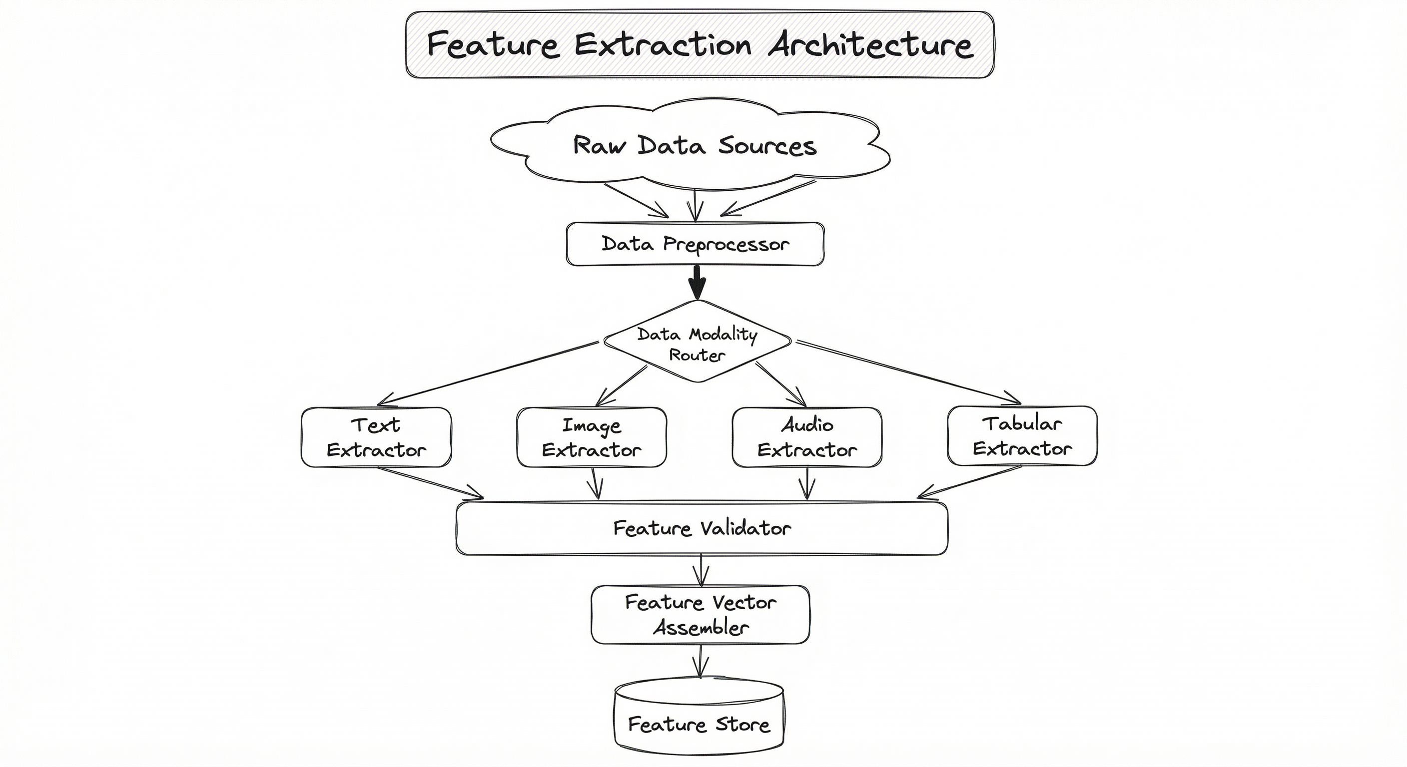
Feature Extraction in ML Systems Architecture — A flowchart showing raw data sources flowing into a data preprocessor, then branching via a modal...

The modality router is a critical design decision. In multimodal systems -- think a food delivery app like Swiggy that processes restaurant images, menu text, and user review audio -- you need parallel extraction pipelines that produce compatible output dimensions for downstream fusion. The feature vector assembler concatenates, stacks, or projects these modality-specific features into a unified representation.

Key Components

Data Preprocessor

Handles modality-specific preprocessing before feature extraction: tokenization and lowercasing for text, resizing and normalization for images, resampling and windowing for audio, type casting and null handling for tabular data. This stage ensures all inputs conform to the expected format for their respective extractors.

Modality Router

Routes each data sample to the appropriate feature extractor based on its type. In multimodal systems, a single sample may be routed to multiple extractors simultaneously (e.g., a product listing has both image and text).

Text Feature Extractor

Converts text into numerical features. Classical options include Bag of Words, TF-IDF, and n-gram representations. Modern options include Word2Vec, GloVe, FastText (static embeddings), and BERT, Sentence-BERT (contextual embeddings). The choice depends on compute budget, corpus size, and task requirements.

Image Feature Extractor

Converts images into feature vectors. Classical options include SIFT, HOG, and color histograms. Modern options use transfer learning from pre-trained CNNs (ResNet, EfficientNet) or Vision Transformers (ViT, DINOv2). The penultimate layer activations of a frozen pre-trained model are the most common approach.

Audio Feature Extractor

Converts audio waveforms into features. Classical options include MFCCs, spectral features (centroid, bandwidth, rolloff), and chroma features. Modern options include learned representations from wav2vec 2.0, HuBERT, or Whisper encoder outputs.

Tabular Feature Extractor

Generates features from structured data. Includes creating interaction features (ratios, products), temporal features (time-since-event, rolling aggregates), encoding categorical variables (one-hot, target encoding), and applying dimensionality reduction (PCA, autoencoders) to high-dimensional numeric columns.

Feature Validator

Checks extracted features for quality issues: NaN/Inf values, unexpected dimensionality, distribution drift from training statistics, and feature value range violations. Critical for catching silent bugs in extraction pipelines.

Feature Vector Assembler

Combines features from multiple extractors into a single feature vector. May concatenate, apply learned fusion (attention-based merging), or project into a shared embedding space for multimodal systems.

Data Flow

Offline (Training) Path: Raw data is pulled from data lakes or warehouses -> preprocessed in batch -> routed to modality-specific extractors -> validated -> assembled into feature vectors -> stored in a feature store (e.g., Feast, Tecton) or directly consumed by model training jobs. Batch extraction typically runs on Spark, Dask, or Ray for parallelism.

Online (Serving) Path: Incoming request data is preprocessed -> features extracted in real-time (or looked up from a precomputed feature store) -> assembled -> sent to the model serving endpoint. Online extraction must meet strict latency SLAs (typically <50ms for feature computation). Pre-trained model inference (e.g., BERT embedding) is the most expensive step and often requires GPU or model distillation.

Key Design Principle: Feature extraction logic must be identical between training and serving to avoid training-serving skew -- one of the most common and insidious bugs in production ML. Use shared extraction code, or better yet, a feature store that guarantees consistency.

A flowchart showing raw data sources flowing into a data preprocessor, then branching via a modality router into four parallel paths (text, image, audio, tabular feature extractors), each converging into a feature validator, then a feature vector assembler, and finally outputting to a feature store or training pipeline.

How to Implement

Implementation Approaches by Modality

Feature extraction implementation varies dramatically by data modality. Let us walk through the most common patterns:

Text: For classical features, scikit-learn's TfidfVectorizer and CountVectorizer are the gold standard -- battle-tested, fast, and production-ready. For learned embeddings, Hugging Face's transformers library provides access to hundreds of pre-trained models. The key decision is sparse vs. dense: TF-IDF produces sparse vectors (fast, interpretable, memory-efficient) while BERT produces dense vectors (richer semantics, higher compute cost).

Images: torchvision pre-trained models (ResNet, EfficientNet, ViT) are the standard for CNN-based feature extraction. Use torch.no_grad() for inference, and extract features from the penultimate layer (before the classification head). For classical features, OpenCV provides SIFT, ORB, and histogram functions.

Audio: librosa is the de facto library for MFCC and spectral feature extraction. For learned audio features, torchaudio provides access to wav2vec 2.0 and HuBERT models.

Tabular: featuretools automates feature generation from relational datasets using Deep Feature Synthesis. tsfresh extracts hundreds of time-series features automatically. For manual feature engineering, pandas and numpy remain the workhorses.

Cost Note: Running BERT feature extraction over 1 million documents on a single NVIDIA T4 GPU (available on AWS at ~ $0.53/hour or ~INR 44/hour) takes approximately 4-6 hours, costing roughly$ 3 (~INR 250). The same task with TF-IDF on a 4-core CPU takes under 5 minutes and costs almost nothing. Choose wisely based on your quality requirements and budget.

TF-IDF Feature Extraction with scikit-learn35 lines

from sklearn.feature_extraction.text import TfidfVectorizer
import numpy as np

# Corpus of documents
documents = [
    "Flipkart offers great deals on electronics",
    "Swiggy delivers food from restaurants near you",
    "Razorpay processes online payments securely",
    "Zomato provides restaurant reviews and ratings",
    "PhonePe enables UPI-based digital payments"
]

# Configure TF-IDF extractor
tfidf = TfidfVectorizer(
    max_features=5000,       # Limit vocabulary size
    min_df=1,                # Minimum document frequency
    max_df=0.95,             # Remove terms in >95% of docs
    ngram_range=(1, 2),      # Unigrams and bigrams
    sublinear_tf=True,       # Apply log normalization to TF
    strip_accents='unicode'
)

# Fit and transform
tfidf_matrix = tfidf.fit_transform(documents)

print(f"Feature matrix shape: {tfidf_matrix.shape}")  # (5, N)
print(f"Vocabulary size: {len(tfidf.vocabulary_)}")
print(f"Sparsity: {1 - tfidf_matrix.nnz / np.prod(tfidf_matrix.shape):.2%}")

# Get feature names for interpretability
feature_names = tfidf.get_feature_names_out()
for i, doc in enumerate(documents):
    top_indices = tfidf_matrix[i].toarray().argsort()[0][-5:]
    top_features = [(feature_names[j], tfidf_matrix[i, j]) for j in top_indices]
    print(f"\nDoc {i}: {top_features}")

This example demonstrates TF-IDF feature extraction, the most widely used classical text featurization method. The sublinear_tf=True flag applies logarithmic scaling to term frequencies, preventing long documents from dominating. The ngram_range=(1, 2) captures both individual words and two-word phrases, which is important for capturing phrases like 'online payments' or 'food delivery'. TF-IDF produces sparse vectors, which are memory-efficient and work well with linear models like logistic regression and SVM.

CNN Feature Extraction with Pre-trained ResNet (PyTorch)48 lines

import torch
import torchvision.models as models
import torchvision.transforms as transforms
from PIL import Image
import numpy as np

# Load pre-trained ResNet-50 and remove classification head
resnet = models.resnet50(weights=models.ResNet50_Weights.IMAGENET1K_V2)
feature_extractor = torch.nn.Sequential(*list(resnet.children())[:-1])  # Remove final FC layer
feature_extractor.eval()

# Define preprocessing (must match ImageNet training)
preprocess = transforms.Compose([
    transforms.Resize(256),
    transforms.CenterCrop(224),
    transforms.ToTensor(),
    transforms.Normalize(mean=[0.485, 0.456, 0.406],
                         std=[0.229, 0.224, 0.225]),
])

def extract_image_features(image_path: str) -> np.ndarray:
    """Extract 2048-dim features from an image using ResNet-50."""
    img = Image.open(image_path).convert('RGB')
    img_tensor = preprocess(img).unsqueeze(0)  # Add batch dimension
    
    with torch.no_grad():
        features = feature_extractor(img_tensor)
    
    return features.squeeze().numpy()  # Shape: (2048,)

# Example usage
features = extract_image_features('product_image.jpg')
print(f"Feature vector shape: {features.shape}")   # (2048,)
print(f"Feature vector norm: {np.linalg.norm(features):.4f}")

# For batch extraction (more efficient)
def extract_batch_features(image_paths: list, batch_size: int = 32) -> np.ndarray:
    """Extract features for a batch of images."""
    all_features = []
    for i in range(0, len(image_paths), batch_size):
        batch_paths = image_paths[i:i + batch_size]
        batch_tensors = torch.stack([
            preprocess(Image.open(p).convert('RGB')) for p in batch_paths
        ])
        with torch.no_grad():
            batch_features = feature_extractor(batch_tensors)
        all_features.append(batch_features.squeeze(-1).squeeze(-1).numpy())
    return np.vstack(all_features)

This example shows the most common production pattern for image feature extraction: using a pre-trained CNN (ResNet-50) as a frozen feature extractor. By removing the final classification layer, we get 2048-dimensional feature vectors that encode rich visual information -- edges, textures, shapes, and high-level object concepts learned from ImageNet. This approach is used at Flipkart for visual product search and at countless other companies for image similarity, duplicate detection, and visual recommendation. The batch extraction function is critical for processing large catalogs efficiently.

MFCC Audio Feature Extraction with librosa49 lines

import librosa
import numpy as np

def extract_audio_features(audio_path: str, sr: int = 22050, n_mfcc: int = 13) -> dict:
    """Extract comprehensive audio features from a WAV file."""
    # Load audio
    y, sr = librosa.load(audio_path, sr=sr)
    
    # 1. MFCCs (most important for speech/music)
    mfccs = librosa.feature.mfcc(y=y, sr=sr, n_mfcc=n_mfcc)
    mfcc_mean = np.mean(mfccs, axis=1)     # Mean across time
    mfcc_std = np.std(mfccs, axis=1)        # Std across time
    mfcc_delta = librosa.feature.delta(mfccs)
    mfcc_delta_mean = np.mean(mfcc_delta, axis=1)
    
    # 2. Spectral features
    spectral_centroid = np.mean(librosa.feature.spectral_centroid(y=y, sr=sr))
    spectral_bandwidth = np.mean(librosa.feature.spectral_bandwidth(y=y, sr=sr))
    spectral_rolloff = np.mean(librosa.feature.spectral_rolloff(y=y, sr=sr))
    zero_crossing_rate = np.mean(librosa.feature.zero_crossing_rate(y))
    
    # 3. Chroma features (pitch classes)
    chroma = librosa.feature.chroma_stft(y=y, sr=sr)
    chroma_mean = np.mean(chroma, axis=1)   # 12 pitch classes
    
    # 4. RMS energy
    rms = np.mean(librosa.feature.rms(y=y))
    
    # Combine into a single feature vector
    feature_vector = np.concatenate([
        mfcc_mean,           # 13 features
        mfcc_std,            # 13 features
        mfcc_delta_mean,     # 13 features
        chroma_mean,         # 12 features
        [spectral_centroid, spectral_bandwidth, spectral_rolloff,
         zero_crossing_rate, rms]  # 5 features
    ])
    
    return {
        'feature_vector': feature_vector,  # Shape: (56,)
        'mfccs_full': mfccs,               # Shape: (13, T)
        'sample_rate': sr,
        'duration_sec': len(y) / sr
    }

# Example usage
result = extract_audio_features('speech_sample.wav')
print(f"Feature vector shape: {result['feature_vector'].shape}")  # (56,)
print(f"Audio duration: {result['duration_sec']:.2f}s")

This example extracts a comprehensive set of audio features using librosa. MFCCs are the most important features for speech and music analysis -- they approximate the human auditory system's response by mapping frequencies to the mel scale. We extract not just the raw MFCCs but also their statistics (mean, std) and first-order deltas (capturing temporal dynamics). Spectral features provide additional information about the frequency distribution. Chroma features capture pitch class information, useful for music analysis. The final 56-dimensional feature vector is compact enough for traditional classifiers yet rich enough for many audio classification tasks.

PCA for Dimensionality Reduction / Feature Extraction33 lines

from sklearn.decomposition import PCA
from sklearn.preprocessing import StandardScaler
import numpy as np
import matplotlib.pyplot as plt

# Simulate high-dimensional tabular data (e.g., 500 features from sensors)
np.random.seed(42)
X = np.random.randn(10000, 500)
# Add some correlated features (realistic scenario)
X[:, 100:200] = X[:, :100] + np.random.randn(10000, 100) * 0.1
X[:, 200:300] = X[:, :100] * 0.5 + np.random.randn(10000, 100) * 0.3

# Step 1: Always standardize before PCA
scaler = StandardScaler()
X_scaled = scaler.fit_transform(X)

# Step 2: Fit PCA and find optimal number of components
pca_full = PCA()
pca_full.fit(X_scaled)

# Find number of components for 95% variance
cumulative_variance = np.cumsum(pca_full.explained_variance_ratio_)
n_components_95 = np.argmax(cumulative_variance >= 0.95) + 1
print(f"Components for 95% variance: {n_components_95} (out of {X.shape[1]})")

# Step 3: Extract features with optimal components
pca = PCA(n_components=n_components_95)
X_features = pca.fit_transform(X_scaled)

print(f"Original dimensions: {X.shape[1]}")
print(f"Extracted features: {X_features.shape[1]}")
print(f"Compression ratio: {X.shape[1] / X_features.shape[1]:.1f}x")
print(f"Variance retained: {pca.explained_variance_ratio_.sum():.4f}")

PCA is the most widely used linear feature extraction method. It projects data onto the directions of maximum variance, effectively compressing the information into fewer dimensions. The key steps are: (1) standardize the data (PCA is sensitive to scale), (2) determine the optimal number of components using the cumulative explained variance ratio, and (3) transform the data. In this example, correlated features allow PCA to achieve significant compression. In production, PCA is commonly applied to reduce the dimensionality of sensor data, financial indicators, or as a preprocessing step before clustering.

Pre-trained BERT Embeddings as Features (Hugging Face)51 lines

from transformers import AutoTokenizer, AutoModel
import torch
import numpy as np

# Load pre-trained BERT model and tokenizer
model_name = 'sentence-transformers/all-MiniLM-L6-v2'  # 384-dim, fast
tokenizer = AutoTokenizer.from_pretrained(model_name)
model = AutoModel.from_pretrained(model_name)
model.eval()

def mean_pooling(model_output, attention_mask):
    """Apply mean pooling to token embeddings, respecting padding."""
    token_embeddings = model_output[0]  # First element: token embeddings
    input_mask_expanded = attention_mask.unsqueeze(-1).expand(token_embeddings.size()).float()
    return torch.sum(token_embeddings * input_mask_expanded, 1) / torch.clamp(
        input_mask_expanded.sum(1), min=1e-9
    )

def extract_text_embeddings(texts: list, batch_size: int = 32) -> np.ndarray:
    """Extract sentence embeddings from a list of texts."""
    all_embeddings = []
    
    for i in range(0, len(texts), batch_size):
        batch = texts[i:i + batch_size]
        encoded = tokenizer(batch, padding=True, truncation=True,
                           max_length=512, return_tensors='pt')
        
        with torch.no_grad():
            outputs = model(**encoded)
        
        embeddings = mean_pooling(outputs, encoded['attention_mask'])
        # L2 normalize
        embeddings = torch.nn.functional.normalize(embeddings, p=2, dim=1)
        all_embeddings.append(embeddings.numpy())
    
    return np.vstack(all_embeddings)

# Example: Extract features for product descriptions
texts = [
    "Premium basmati rice 5kg pack for Indian cooking",
    "Wireless Bluetooth earbuds with noise cancellation",
    "Organic cold-pressed coconut oil for hair and skin"
]

embeddings = extract_text_embeddings(texts)
print(f"Embedding shape: {embeddings.shape}")  # (3, 384)

# Compute pairwise cosine similarity
from sklearn.metrics.pairwise import cosine_similarity
sim_matrix = cosine_similarity(embeddings)
print(f"\nSimilarity matrix:\n{sim_matrix}")

This example uses a pre-trained Sentence Transformer model (all-MiniLM-L6-v2) to extract dense 384-dimensional embeddings from text. Unlike TF-IDF, these embeddings capture semantic meaning -- texts about similar topics will have similar embeddings even if they share no words. The mean_pooling function averages token-level embeddings (respecting padding masks) to produce sentence-level representations. L2 normalization ensures cosine similarity can be computed as a simple dot product. This approach is used extensively in production for semantic search, product matching, and recommendation systems.

Autoencoder for Tabular Feature Extraction (PyTorch)81 lines

import torch
import torch.nn as nn
import numpy as np
from sklearn.preprocessing import StandardScaler
from torch.utils.data import DataLoader, TensorDataset

class TabularAutoencoder(nn.Module):
    """Autoencoder for extracting compressed features from tabular data."""
    def __init__(self, input_dim: int, latent_dim: int = 32):
        super().__init__()
        self.encoder = nn.Sequential(
            nn.Linear(input_dim, 256),
            nn.BatchNorm1d(256),
            nn.ReLU(),
            nn.Dropout(0.2),
            nn.Linear(256, 128),
            nn.BatchNorm1d(128),
            nn.ReLU(),
            nn.Dropout(0.2),
            nn.Linear(128, latent_dim),
        )
        self.decoder = nn.Sequential(
            nn.Linear(latent_dim, 128),
            nn.BatchNorm1d(128),
            nn.ReLU(),
            nn.Linear(128, 256),
            nn.BatchNorm1d(256),
            nn.ReLU(),
            nn.Linear(256, input_dim),
        )
    
    def forward(self, x):
        z = self.encoder(x)
        x_hat = self.decoder(z)
        return x_hat, z
    
    def extract_features(self, x):
        """Extract latent features without decoding."""
        self.eval()
        with torch.no_grad():
            return self.encoder(x).numpy()

# Training function
def train_autoencoder(X_train: np.ndarray, latent_dim: int = 32,
                      epochs: int = 100, batch_size: int = 256, lr: float = 1e-3):
    scaler = StandardScaler()
    X_scaled = scaler.fit_transform(X_train)
    
    dataset = TensorDataset(torch.FloatTensor(X_scaled))
    loader = DataLoader(dataset, batch_size=batch_size, shuffle=True)
    
    model = TabularAutoencoder(X_train.shape[1], latent_dim)
    optimizer = torch.optim.Adam(model.parameters(), lr=lr)
    criterion = nn.MSELoss()
    
    for epoch in range(epochs):
        total_loss = 0
        model.train()
        for (batch,) in loader:
            x_hat, z = model(batch)
            loss = criterion(x_hat, batch)
            optimizer.zero_grad()
            loss.backward()
            optimizer.step()
            total_loss += loss.item()
        
        if (epoch + 1) % 20 == 0:
            avg_loss = total_loss / len(loader)
            print(f"Epoch {epoch+1}/{epochs}, Loss: {avg_loss:.6f}")
    
    return model, scaler

# Example usage
X = np.random.randn(10000, 200)  # 200 raw features
model, scaler = train_autoencoder(X, latent_dim=32, epochs=100)

# Extract 32-dim features from new data
X_new = np.random.randn(100, 200)
X_new_scaled = torch.FloatTensor(scaler.transform(X_new))
features = model.extract_features(X_new_scaled)
print(f"Extracted features shape: {features.shape}")  # (100, 32)

This autoencoder compresses 200 raw tabular features into 32 latent dimensions. The encoder learns a nonlinear compression that preserves the most reconstructable information -- think of it as a nonlinear generalization of PCA. Batch normalization stabilizes training, and dropout prevents the encoder from simply memorizing the identity function. In production, this approach is valuable when you have high-dimensional tabular data (sensor readings, user behavior logs, financial indicators) and want to reduce dimensionality while capturing nonlinear relationships that PCA would miss. Razorpay and similar fintech companies use autoencoder-based features for anomaly detection in transaction data.

Automated Feature Extraction with tsfresh (Time Series)35 lines

import pandas as pd
import numpy as np
from tsfresh import extract_features
from tsfresh.feature_extraction import MinimalFCParameters
from tsfresh.utilities.dataframe_functions import impute

# Create sample time series data (e.g., sensor readings per device)
np.random.seed(42)
data = []
for device_id in range(100):
    n_points = np.random.randint(50, 200)
    timestamps = np.arange(n_points)
    values = np.sin(timestamps * 0.1 + device_id) + np.random.randn(n_points) * 0.3
    for t, v in zip(timestamps, values):
        data.append({'id': device_id, 'time': t, 'value': v})

df = pd.DataFrame(data)

# Extract features automatically
# MinimalFCParameters for speed; use ComprehensiveFCParameters for full extraction
extracted = extract_features(
    df,
    column_id='id',
    column_sort='time',
    default_fc_parameters=MinimalFCParameters(),
    n_jobs=4  # Parallelize across CPU cores
)

# Handle NaN/Inf values
impute(extracted)

print(f"Input: {len(df)} rows across {df['id'].nunique()} time series")
print(f"Extracted: {extracted.shape[1]} features per time series")
print(f"Output shape: {extracted.shape}")
print(f"\nSample feature names: {list(extracted.columns[:10])}")

tsfresh automates the extraction of hundreds of statistical features from time series data: mean, variance, autocorrelation, spectral entropy, number of peaks, and many more. The MinimalFCParameters preset extracts a focused set of ~10 features for speed; ComprehensiveFCParameters extracts 700+ features but takes longer. This is particularly valuable for IoT and manufacturing use cases common in India's growing Industry 4.0 sector, where thousands of sensor time series need to be converted into tabular features for anomaly detection, predictive maintenance, or classification.

Configuration Example56 lines

# Feature extraction pipeline config (YAML)
pipeline:
  name: product-feature-extraction
  version: "2.1.0"

  text_features:
    method: tfidf
    params:
      max_features: 10000
      ngram_range: [1, 2]
      sublinear_tf: true
      max_df: 0.95
      min_df: 3
    # Alternative: pre-trained embeddings
    # method: sentence-transformer
    # model: all-MiniLM-L6-v2
    # batch_size: 64

  image_features:
    method: resnet50
    params:
      weights: IMAGENET1K_V2
      layer: avgpool  # 2048-dim output
      batch_size: 32
      device: cuda:0
    preprocessing:
      resize: 256
      center_crop: 224
      normalize:
        mean: [0.485, 0.456, 0.406]
        std: [0.229, 0.224, 0.225]

  audio_features:
    method: mfcc
    params:
      n_mfcc: 13
      sample_rate: 22050
      include_delta: true
      include_spectral: true

  tabular_features:
    pca:
      n_components: 0.95  # Retain 95% variance
      standardize: true
    aggregations:
      - mean
      - std
      - min
      - max
      - skew

  output:
    format: parquet
    destination: s3://ml-features/product-features/
    feature_store: feast
    ttl_hours: 24

Common Implementation Mistakes

●
Not standardizing before PCA: PCA finds directions of maximum variance. If features are on different scales (e.g., age in years vs. income in lakhs), the high-magnitude features dominate. Always apply StandardScaler before PCA. This is the single most common PCA mistake.
●
Using TF-IDF without tuning max_df and min_df: Default settings include extremely common words (noise) and extremely rare words (overfitting risk). Set max_df=0.95 to remove words appearing in >95% of documents and min_df=2-5 to remove words appearing in fewer than a few documents.
●
Extracting CNN features without matching the preprocessing pipeline: Pre-trained ImageNet models expect specific normalization (mean=[0.485, 0.456, 0.406], std=[0.229, 0.224, 0.225]). Using different normalization produces garbage features with no error message. Always check the model card.
●
Training-serving skew in feature extraction: Using one extraction pipeline during training (e.g., a fitted TF-IDF vectorizer with its vocabulary) and a different one during serving. The vocabulary, scaling parameters, and PCA projection matrix must be exactly the same. Serialize the entire pipeline, not just the model.
●
Ignoring the curse of dimensionality with Bag of Words: A naive BoW on a large corpus can produce 100K+ dimensional sparse vectors. Without dimensionality reduction (hashing trick, SVD, or max_features), downstream models become slow and prone to overfitting.
●
Applying autoencoders when PCA suffices: Autoencoders are powerful but harder to train, tune, and deploy. If the relationships in your data are approximately linear, PCA will achieve comparable compression with zero training and perfect reproducibility. Start with PCA, move to autoencoders only when you have evidence of nonlinear structure.
●
Forgetting to handle variable-length inputs: Audio clips have different durations, documents have different lengths, time series have different numbers of observations. Feature extraction must produce fixed-length output. Use pooling (mean, max), padding/truncation, or summary statistics to handle this.

When Should You Use This?

Use When

Your raw data is high-dimensional and needs compression before model training (e.g., 10,000 pixel features reduced to 2,048 CNN features)
You are working with unstructured data (text, images, audio) that cannot be directly consumed by ML models
Your downstream model is a classical algorithm (logistic regression, XGBoost, SVM) that benefits from well-engineered input features rather than raw data
You need interpretable features for debugging, compliance, or stakeholder communication (TF-IDF, handcrafted tabular features)
Transfer learning is viable: a pre-trained model on a large dataset (ImageNet, BookCorpus) can provide useful features for your smaller, domain-specific task
You need to reduce compute cost at inference time by precomputing features offline and serving from a feature store
Your dataset is small and you cannot afford to train deep models end-to-end -- extracted features from pre-trained models provide a strong starting point
You are building a multimodal system and need to project different data types into compatible feature spaces

Avoid When

You have enough labeled data and compute to train an end-to-end deep learning model that learns features internally (e.g., a fine-tuned BERT for text classification with 100K+ labeled examples)
The task is well-suited to end-to-end architectures where learned features outperform handcrafted ones (e.g., image generation, machine translation)
Feature extraction would introduce an information bottleneck that hurts performance -- some tasks need raw pixel/token-level information
Your data is already in a suitable numerical format with low dimensionality (e.g., 10 well-defined tabular columns -- just use them directly)
The extraction process is too slow for your real-time latency requirements and you cannot precompute features (though distillation or caching often solves this)
You are working with very small datasets where even simple feature extraction might overfit (e.g., PCA on 50 samples with 500 features will produce meaningless components)

Key Tradeoffs

The Fundamental Tradeoff: Expressiveness vs. Cost

Every feature extraction method lives on a spectrum between cheap but limited and expensive but powerful:

Method	Compute Cost	Feature Quality	Interpretability	Training Needed
Bag of Words	Very Low	Low-Medium	High	No
TF-IDF	Low	Medium	High	No (just fitting)
PCA	Low-Medium	Medium	Medium	Yes (fit)
MFCC	Low	Medium-High	Medium	No
Word2Vec/GloVe	Medium	Medium-High	Low	Pre-trained
Autoencoder	Medium-High	High	Low	Yes
CNN (frozen)	High	Very High	Low	Pre-trained
BERT embedding	Very High	Very High	Low	Pre-trained

The Second Axis: Sparse vs. Dense

TF-IDF and Bag of Words produce sparse feature vectors (mostly zeros). CNN and BERT features produce dense vectors (all non-zero). This has profound implications:

Sparse features are memory-efficient for storage but can be very high-dimensional (10K-100K). They work well with linear models and are fast to compute. They do not capture semantic similarity.
Dense features are lower-dimensional (256-4096) but every dimension is used. They capture semantic relationships and work with any model type. They require more compute to produce.

The India Startup Cost Calculus

For a typical Indian startup operating on a tight budget, here is a practical cost comparison for extracting features from 1 million text documents:

TF-IDF on CPU: ~5 minutes, ~INR 5 ($0.06) on an EC2 m5.xlarge
Sentence-BERT on GPU: ~4 hours, ~INR 200 ($2.40) on an EC2 g4dn.xlarge (T4 GPU)
Full BERT-large on GPU: ~16 hours, ~INR 1,600 ($19) on an EC2 p3.2xlarge (V100 GPU)

The 300x cost difference between TF-IDF and full BERT makes the choice obvious for many use cases. Start with TF-IDF, measure performance, and upgrade to learned embeddings only if the accuracy gap justifies the cost.

Rule of Thumb: Use the simplest feature extraction method that meets your accuracy requirements. Complexity has a cost -- not just in compute, but in debugging, maintenance, and operational risk.

Alternatives & Comparisons

Feature Selection

Feature extraction creates new features by transforming raw data (e.g., PCA projects into a new space). Feature selection chooses a subset of existing features without transformation. Use feature selection when your original features are already meaningful and you just need to remove redundant or irrelevant ones. Use feature extraction when raw data needs to be transformed into a usable format.

Embedding Model (End-to-End)

An embedding model trained end-to-end (e.g., fine-tuned BERT, CLIP) learns features optimized for a specific task. Standalone feature extraction uses frozen, task-agnostic representations. End-to-end embeddings are more powerful when you have sufficient labeled data and compute. Feature extraction with pre-trained models is better when data is scarce or compute is limited.

Data Transformation

Data transformation (normalization, scaling, encoding) prepares existing features for model consumption without creating fundamentally new representations. Feature extraction creates new representations from raw data. They are complementary: you often transform data first (clean, scale), then extract features, then transform again (normalize the extracted features).

Categorical Encoding

Categorical encoding (one-hot, label, target encoding) converts categorical variables into numbers. Feature extraction is broader -- it includes encoding but also encompasses transformation of unstructured data (text, images, audio) and dimensionality reduction. Encoding is a subset of the feature extraction toolkit.

Pros, Cons & Tradeoffs

Advantages

Enables ML on unstructured data: Without feature extraction, you simply cannot apply classical ML algorithms to text, images, or audio. It is the bridge between raw signal and model-ready input.
Dramatic dimensionality reduction: PCA can compress 10,000 features to 100 while retaining 95% of variance. CNN features compress 150K pixel values to 2,048. This reduction speeds up training by orders of magnitude.
Transfer learning leverage: Pre-trained feature extractors (ResNet, BERT) encode billions of parameters worth of learned knowledge. You get the benefit of training on ImageNet or BookCorpus without the compute cost (~$50K+ to train BERT from scratch).
Improved model generalization: Well-extracted features reduce noise and irrelevant variation, making it easier for downstream models to learn robust patterns rather than memorizing artifacts.
Interpretability of classical features: TF-IDF weights, PCA loadings, and handcrafted tabular features are inspectable and explainable -- critical for regulated industries like banking (RBI compliance in India) and healthcare.
Decouples feature computation from model training: Features can be precomputed, cached, and reused across multiple models and experiments. This is the foundation of the feature store pattern used at companies like Uber, Airbnb, and Flipkart.
Works with small datasets: Pre-trained feature extractors provide strong representations even when you have only hundreds of labeled examples -- a common scenario in Indian enterprise ML where labeled data is expensive.

Disadvantages

Information loss is inevitable: Every feature extraction method discards some information. PCA drops low-variance directions. TF-IDF drops word order. CNN pooling drops spatial precision. If the discarded information matters for your task, performance will suffer.
Training-serving skew risk: The feature extraction pipeline must be identical between training and serving. Drift in preprocessing, vocabulary, or scaling parameters silently degrades model quality with no error messages.
Computational cost for deep features: Extracting BERT or CNN features at scale requires GPUs. For 100M documents, BERT extraction on V100 GPUs costs approximately INR 1.5-2 lakh ( $1,800-$ 2,400) -- a significant expense for startups.
Maintenance burden: Feature extraction code becomes the most fragile part of the pipeline. Changes to tokenization, image resizing, or audio sampling break downstream models. Every extractor is a contract you must maintain.
Feature staleness: Precomputed features become stale when the underlying data changes or when the extraction method is updated. Re-extraction for large corpora is expensive and time-consuming.
Curse of dimensionality with naive methods: Bag of Words on large vocabularies produces extremely sparse, high-dimensional vectors that cause memory issues and degrade model performance. Without careful tuning, you trade one problem for another.
Hyperparameter sensitivity: PCA requires choosing the number of components. TF-IDF requires tuning max_features, min_df, max_df, and ngram_range. Autoencoders require architecture design, learning rate, and regularization choices. Getting these wrong can be worse than using raw features.

Start with small batch sizes (16-32) and increase gradually. Use torch.no_grad() to disable gradient computation (halves memory usage). Process in streaming fashion rather than loading all data into memory. Use mixed precision (torch.float16) for 2x memory savings with minimal quality loss. For very large corpora, use distributed extraction across multiple GPUs or nodes.

Placement in an ML System

Where Feature Extraction Fits

Feature extraction sits in the Feature Engineering stage of the ML pipeline, between data preprocessing (cleaning, normalization) and model training. It is the step that transforms human-readable data into model-readable numerical representations.

In a training pipeline: Raw data -> Clean/Preprocess -> Feature Extraction -> Feature Selection (optional) -> Feature Store (optional) -> Model Training. The feature extractor is typically fit/configured on training data and its parameters are frozen for inference.

In a serving pipeline: Incoming request -> Feature Extraction (real-time or lookup from feature store) -> Model Inference -> Response. Feature extraction latency directly impacts end-to-end inference latency. For Swiggy's restaurant ranking model, feature extraction (computing user preference features, restaurant features, and contextual features) must complete in under 50ms to meet their SLA.

In batch pipelines: Feature extraction runs as a scheduled job (hourly, daily) that precomputes features for a large corpus and stores them in a feature store. This is the dominant pattern for recommendation systems at scale -- Flipkart precomputes product features, user features, and interaction features in batch, then joins them at serving time.

Critical Insight: Feature extraction quality directly determines the ceiling of model performance. If important information is lost during extraction, no amount of model tuning can recover it. This is why senior ML engineers spend more time on feature extraction than on model architecture.

Pipeline Stage

Feature Engineering

Upstream

data-transformation
data-preprocessing
data-cleaning

Downstream

feature-selection
feature-store
model-training
scaling

Scaling Bottlenecks

Where Feature Extraction Gets Tight

The primary bottleneck depends on the extraction method:

CPU-bound methods (TF-IDF, PCA, MFCC): Scale linearly with data volume. A TF-IDF extraction over 100M documents takes ~8 hours on a 32-core machine. Mitigation: parallelize with Spark or Dask. PCA becomes memory-bound for very wide matrices ( $p > 50K$ ) because the covariance matrix is $p \times p$ .

GPU-bound methods (CNN, BERT): Scale linearly with data volume and are constrained by GPU memory and throughput. A single V100 GPU processes ~500 images/second through ResNet-50 or ~100 sentences/second through BERT-base. Mitigation: multi-GPU parallelism, model distillation (DistilBERT is 60% faster than BERT-base with 97% of the quality), or batch processing on spot instances.

Storage bottleneck: Dense feature vectors consume significant storage. 100M documents x 768 dimensions x 4 bytes = ~300 GB. With multiple feature versions (for A/B testing or model comparison), storage costs multiply. Mitigation: quantize features to float16 (halves storage), use columnar formats (Parquet), or implement a feature store with garbage collection.

Some concrete numbers for Indian cloud pricing: extracting CNN features for 10M product images on AWS g4dn.xlarge (T4 GPU, ~INR 50/hour) takes approximately 6 hours, costing ~INR 300 ( $3.60). The same on an `m5.4xlarge` CPU instance takes ~60 hours and costs ~INR 4,800 ($ 57). GPUs are almost always cheaper for deep feature extraction at scale.

Production Case Studies

FlipkartE-commerce (India)

Flipkart built VisNet, a deep CNN trained using a triplet-based deep ranking paradigm for visual product search. The system extracts image features using a VGG-16-based architecture coupled with parallel shallow convolution layers to capture both high-level semantic and low-level visual details from product catalog images. These features power visual similarity search across 50 million+ product listings, enabling users to find visually similar products by uploading a photo.

Outcome:

Achieved state-of-the-art results on the Street2Shop benchmark. The system processes 100K+ catalog additions/deletions per hour and serves visual recommendations to over 100 million users. Feature extraction reduced the visual search problem from comparing raw images (~150K pixels) to comparing compact feature vectors (~2048 dimensions), making real-time retrieval feasible.

RazorpayFintech (India)

Razorpay's Thirdwatch fraud detection system extracts hundreds of features from transaction data in real-time using Apache Flink. Features include device fingerprinting signals (proxy IP, device ID), behavioral signals (time to order, browsing patterns), and derived features (price-to-device-value ratio, address quality scores). The system uses Flink's in-memory states and complex event processing (CEP) to compute rolling aggregation features with sub-200ms latency.

Outcome:

Real-time feature extraction enables fraud evaluation within milliseconds, reducing fraud rates while preserving transaction success rates. The system processes millions of transactions daily, extracting and serving ML features to models that generate risk scores for every payment.

NetflixStreaming Entertainment

Netflix's recommendation system extracts features across multiple modalities: user behavior features (watch history, ratings, time-of-day patterns), content features (genre embeddings, visual features from thumbnails, NLP features from synopses), and contextual features (device type, time, region). Their feature engineering pipeline transforms raw behavioral data into model-ready representations in real-time, computing user preference vectors, content similarity matrices, and contextual embeddings that update continuously.

Outcome:

Netflix's recommendation system generates over 80% of watched content through personalized suggestions. The multi-modal feature extraction approach enables them to consolidate dozens of specialized models into a more maintainable unified architecture while maintaining recommendation quality across 200M+ subscribers.

UberRide-sharing & Delivery

Uber's Michelangelo ML platform includes a comprehensive feature extraction and storage system. Features are extracted from diverse sources: real-time trip data, historical ride patterns, geospatial features (distance to landmarks, neighborhood characteristics), and temporal features (time-of-day, day-of-week, holiday indicators). The platform automates feature computation at both batch (Spark) and real-time (Flink) scales, storing results in a unified feature store.

Outcome:

Michelangelo's standardized feature extraction pipeline reduced the time to deploy new ML models from months to weeks. The feature store serves features for hundreds of ML models across ETA prediction, dynamic pricing, fraud detection, and demand forecasting, processing millions of feature lookups per second.

SpotifyMusic Streaming

Spotify extracts both audio features (MFCCs, spectral features, tempo, loudness) and text features (NLP embeddings from podcast transcripts, song metadata, playlist descriptions) to power discovery and recommendation. For their natural language podcast search, they extract BERT-based semantic embeddings from episode transcripts and user queries, enabling semantic matching between spoken content and search intent.

Outcome:

Audio and text feature extraction enables Spotify to recommend across modalities -- suggesting podcasts based on music taste and vice versa. Their natural language search reduced the gap between user intent and content discovery for 5M+ podcast episodes.

PicnicDelivery

Picnic, a Dutch online grocery delivery service, built a feature engineering pipeline to predict optimal delivery drop times. They extracted features from historical GPS traces, traffic patterns, building types, and customer-specific unloading times to predict how long each delivery stop would take. Key features included stop sequence position, parcel count, floor level, and time-of-day traffic indices (2020).

Outcome:

The ML-based drop time predictions enabled Picnic to optimize route planning accuracy by 20%, reducing both early and late deliveries. The feature pipeline now processes millions of historical data points to maintain prediction accuracy as delivery patterns evolve.

Tooling & Ecosystem

scikit-learn (feature_extraction module)

PythonOpen Source

The de facto standard for classical feature extraction in Python. Provides TfidfVectorizer, CountVectorizer, HashingVectorizer for text; PCA, TruncatedSVD, NMF for dimensionality reduction; and DictVectorizer for tabular data. Battle-tested, well-documented, and integrates seamlessly with sklearn pipelines.

Hugging Face Transformers

PythonOpen Source

Provides access to thousands of pre-trained models (BERT, RoBERTa, ViT, wav2vec) for extracting deep features from text, images, and audio. The pipeline API makes feature extraction a one-liner. Essential for any modern feature extraction workflow involving learned representations.

PyTorch (torchvision, torchaudio)

Python / C++Open Source

PyTorch's ecosystem includes torchvision.models for pre-trained CNN feature extractors (ResNet, EfficientNet, ViT) and torchaudio for audio feature extraction (MFCCs, spectrograms, mel filterbanks). GPU acceleration makes batch extraction fast.

librosa

PythonOpen Source

The standard Python library for audio and music analysis. Provides MFCC, spectral features, chroma features, tempo estimation, and beat tracking. Lightweight, well-documented, and does not require GPUs.

OpenCV

C++ / PythonOpen Source

Comprehensive computer vision library providing classical feature extractors (SIFT, ORB, HOG), image preprocessing, and histogram computation. Essential for handcrafted image features and real-time video processing.

Featuretools

PythonOpen Source

Automates feature engineering from relational and temporal datasets using Deep Feature Synthesis (DFS). Generates interaction features, aggregation features, and transformation features automatically. Developed by Alteryx. Especially useful for tabular ML on transactional data.

tsfresh

PythonOpen Source

Automatic extraction of relevant features from time series data. Computes 700+ statistical features (mean, variance, autocorrelation, spectral entropy, peaks, etc.) and includes built-in feature selection using hypothesis testing. Integrates with scikit-learn and pandas.

Feast (Feature Store)

Python / GoOpen Source

Open-source feature store that manages the lifecycle of extracted features -- from computation to storage to serving. Ensures training-serving consistency for feature extraction pipelines. Critical for operationalizing feature extraction at scale.

Research & References

Efficient Estimation of Word Representations in Vector Space

Mikolov, Chen, Corrado & Dean (2013)ICLR 2013

Introduced Word2Vec (Skip-gram and CBOW architectures) for learning distributed word representations from large text corpora. Demonstrated that learned word vectors capture syntactic and semantic regularities, revolutionizing text feature extraction by replacing sparse BoW features with dense, semantically meaningful embeddings.

BERT: Pre-training of Deep Bidirectional Transformers for Language Understanding

Devlin, Chang, Lee & Toutanova (2019)NAACL 2019

Introduced BERT, which produces context-dependent word representations by pre-training a bidirectional Transformer on masked language modeling. BERT's hidden layer activations serve as powerful feature extractors for downstream NLP tasks, achieving state-of-the-art results across 11 benchmarks.

Deep Residual Learning for Image Recognition

He, Zhang, Ren & Sun (2016)CVPR 2016

Introduced ResNet with skip connections enabling training of very deep CNNs. Pre-trained ResNet models became the standard image feature extractor, with penultimate layer activations providing 2048-dimensional features that transfer effectively across visual domains.

A Tutorial on Principal Component Analysis

Shlens (2014)arXiv preprint

A widely-cited tutorial building intuition for PCA as a feature extraction and dimensionality reduction technique. Covers the mathematical foundations, geometric interpretation, and practical considerations for applying PCA to real datasets.

Automated Data Processing and Feature Engineering for Deep Learning and Big Data Applications: A Survey

Mumuni & Mumuni (2024)arXiv preprint

Comprehensive 2024 survey covering automated feature extraction techniques including AutoML-based approaches, automated data preprocessing, and neural architecture search for feature engineering. Reviews the shift from manual to automated feature extraction pipelines.

Autoencoders and Their Applications in Machine Learning: A Survey

Berahmand, Daneshfar, Salehi, Li & Xu (2024)Artificial Intelligence Review

Comprehensive survey of autoencoder architectures (vanilla, variational, denoising, sparse, contractive) and their applications in feature extraction, dimensionality reduction, and representation learning across domains including image, text, and tabular data.

Deep Learning Based Large Scale Visual Recommendation and Search for E-Commerce

Shankar, Garg, et al. (Flipkart) (2017)arXiv preprint

Describes Flipkart's VisNet system for extracting visual features from product images using deep CNNs. Demonstrates production-scale feature extraction for visual recommendation and search across 50M+ product listings.

An Automated Data Mining Framework Using Autoencoders for Feature Extraction and Dimensionality Reduction

Alkinani, Al-Waisy, Al-Fahdawi & Mohammed (2024)arXiv preprint

Proposes an automated framework combining autoencoders with traditional ML classifiers for feature extraction and dimensionality reduction. Demonstrates effectiveness across multiple datasets with significant improvements in noise reduction and anomaly detection.

Interview & Evaluation Perspective

Common Interview Questions

●
How would you design a feature extraction pipeline for a multimodal recommendation system (text + images + user behavior)?
●
Compare TF-IDF vs. BERT embeddings for text classification. When would you choose each?
●
What is PCA and how does it extract features? What happens if you do not standardize before PCA?
●
How do you handle training-serving skew in feature extraction pipelines?
●
Explain transfer learning for feature extraction. Why does a CNN trained on ImageNet work for medical image classification?
●
How would you design a real-time feature extraction system that meets a 50ms latency SLA?
●
What is the curse of dimensionality and how does feature extraction help mitigate it?
●
How would you extract features from audio data for a speech emotion recognition system?

Key Points to Mention

●
Feature extraction transforms raw data into fixed-dimensional numerical representations. The two major categories are handcrafted (TF-IDF, MFCC, PCA) and learned (CNN, BERT, autoencoders). Always start by identifying which is appropriate for your constraints.
●
Training-serving skew is the #1 production failure mode for feature extraction. The extraction pipeline must be serialized and version-controlled alongside the model. Use a feature store (Feast, Tecton) for consistency.
●
For text: TF-IDF is fast, interpretable, and works well with limited compute. BERT embeddings capture semantic meaning but cost 100x more to compute. The choice depends on accuracy requirements and budget -- quantify the tradeoff.
●
For images: Pre-trained CNN features (ResNet penultimate layer) are the standard approach. The preprocessing must exactly match the model's training preprocessing. Always check the model card.
●
For tabular data: Handcrafted domain features (ratios, rolling aggregates, time-since-event) often outperform automated approaches. PCA is appropriate when you have many correlated numeric features. Autoencoders help when relationships are nonlinear.
●
Cost matters in practice. A senior candidate should be able to estimate extraction costs: BERT over 1M docs on T4 GPU costs ~INR 200, TF-IDF on CPU costs ~INR 5. This shapes real design decisions.

Pitfalls to Avoid

●
Claiming deep features are always better than classical features -- TF-IDF + XGBoost beats BERT + logistic regression on many tabular/small-data tasks. Always benchmark.
●
Ignoring computational cost: suggesting BERT embeddings for a startup with no GPU budget shows lack of practical awareness.
●
Forgetting to mention training-serving skew -- this is the most common production failure and the first thing senior interviewers look for.
●
Treating PCA and feature selection as the same thing -- PCA creates new features through projection; feature selection chooses a subset of existing features.
●
Not discussing how to handle variable-length inputs (padding, truncation, pooling) when extracting features from sequences.

Senior-Level Expectation

A senior/staff candidate should demonstrate end-to-end system thinking: not just which extraction method to use, but how to operationalize it. This includes: (1) feature extraction pipeline architecture with training-serving consistency, (2) cost estimation and optimization (when to use GPUs vs. CPUs, batch vs. real-time), (3) feature versioning and monitoring for drift, (4) the feature store pattern for decoupling extraction from training, (5) multimodal feature fusion strategies, and (6) the ability to reason about the information bottleneck -- what information is lost by each extraction method and whether that loss matters for the task. Senior candidates should also discuss when NOT to extract features -- when end-to-end learning is superior and why.

Summary

Feature extraction is the foundational step that transforms raw, messy, real-world data into the clean numerical representations that ML models require. We have covered the full spectrum of techniques: classical methods (TF-IDF for text, MFCC for audio, PCA for dimensionality reduction, handcrafted tabular features) that are fast, interpretable, and require no training data; and learned methods (CNN features via transfer learning, BERT embeddings, autoencoders) that capture richer representations but demand more compute. The choice between them is not about which is "better" in the abstract -- it is about which meets your specific accuracy, latency, cost, and interpretability requirements.

In production, the key challenges are not the extraction algorithms themselves but the operational concerns: ensuring training-serving consistency (serialized pipelines, feature stores), managing computational cost (GPU vs. CPU, batch vs. real-time, model distillation), handling feature versioning and staleness (periodic re-computation, drift monitoring), and scaling extraction to millions or billions of data points (distributed processing, caching, quantization). Companies like Flipkart, Razorpay, Netflix, Uber, and Spotify have built sophisticated feature extraction platforms to address these challenges at scale.

The most important insight to carry forward is this: feature extraction determines the ceiling of your model's performance. No amount of model tuning, hyperparameter search, or architectural innovation can compensate for features that lose critical information or introduce noise. Invest your time where it matters most -- and for most ML systems, that is in the feature extraction pipeline. Start simple (TF-IDF, PCA), measure rigorously, and upgrade to learned features only when the accuracy gap justifies the cost and complexity.

Concept Snapshot

Why This Concept Exists

Raw Data Is Not Model-Ready

The Evolution: From Handcrafted to Learned Features

Why Handcrafted Features Still Matter

Core Intuition & Mental Model

The Core Promise

Two Fundamental Flavors

The Information Bottleneck View

Technical Foundations

Mathematical Framework

Key Classical Methods

Complexity Considerations

Internal Architecture

Key Components

Data Flow

How to Implement

Implementation Approaches by Modality

Common Implementation Mistakes

When Should You Use This?

Use When

Avoid When

Key Tradeoffs

The Fundamental Tradeoff: Expressiveness vs. Cost

The Second Axis: Sparse vs. Dense

The India Startup Cost Calculus

Alternatives & Comparisons

Pros, Cons & Tradeoffs

Advantages

Disadvantages

Failure Modes & Debugging

Training-Serving Skew

Dimensionality Explosion

Feature Leakage

Preprocessing Mismatch for Pre-trained Models

Stale Features After Data Distribution Shift

GPU Memory Exhaustion During Batch Extraction

Placement in an ML System

Where Feature Extraction Fits

Pipeline Stage

Upstream

Downstream

Scaling Bottlenecks

Production Case Studies

Tooling & Ecosystem

Research & References

Interview & Evaluation Perspective

Common Interview Questions

Key Points to Mention

Pitfalls to Avoid

Senior-Level Expectation

Summary

Related Blocks & Further Reading

Related ML Blocks

Further Reading