Mixup in Machine Learning
Mixup is one of the simplest and most impactful regularization techniques to emerge in modern deep learning. The idea, introduced by Zhang et al. in 2018, is almost embarrassingly straightforward: take two training samples, blend their inputs via a weighted average, and blend their labels with the same weight. Train on the blended pair. That's it.
But the consequences of this simple recipe are profound. Mixup forces neural networks to learn linear behavior between training examples, producing smoother decision boundaries, better-calibrated predictions, and measurably improved robustness to adversarial perturbations and label noise. It acts simultaneously as a data augmentation technique (generating virtual training samples that never existed in your dataset) and as an implicit regularizer (inducing label smoothing and reducing the Lipschitz constant of the learned function).
What makes Mixup particularly compelling for production ML systems is its domain-agnostic nature. Unlike geometric augmentations that only apply to images or back-translation that only works for text, Mixup operates on raw feature vectors and labels -- meaning it transfers to computer vision, NLP, speech, tabular data, and multi-modal settings with minimal modification. From Google's image classification pipelines to medical imaging startups in Bengaluru, Mixup has become a default ingredient in modern training recipes.
This guide covers the original Mixup formulation, the Beta distribution mechanics, Manifold Mixup in hidden layers, extensions to NLP and speech, comparisons with CutMix and Cutout, failure modes in production, and practical implementation patterns you can deploy today.
Concept Snapshot
- What It Is
- A data augmentation and regularization technique that trains neural networks on convex combinations (weighted blends) of pairs of training examples and their labels, encouraging linear behavior between samples.
- Category
- Data Generation
- Complexity
- Beginner
- Inputs / Outputs
- Inputs: pairs of training examples $(x_i, y_i)$ and $(x_j, y_j)$ with a mixing coefficient $\lambda$ sampled from a Beta distribution. Outputs: virtual training pair $(\tilde{x}, \tilde{y})$ where $\tilde{x} = \lambda x_i + (1-\lambda) x_j$ and $\tilde{y} = \lambda y_i + (1-\lambda) y_j$.
- System Placement
- Applied during training data loading, typically in the data loader or collate function. Operates on mini-batches before they are fed to the model. Not used at inference time (though test-time Mixup variants exist).
- Also Known As
- input mixup, vanilla mixup, linear interpolation augmentation, convex combination augmentation, sample mixing
- Typical Users
- ML engineers, Deep learning researchers, Computer vision practitioners, NLP engineers, Data scientists
- Prerequisites
- Basic neural network training (loss functions, backpropagation), One-hot encoding and soft labels, Overfitting and regularization concepts, Probability distributions (Beta distribution basics)
- Key Terms
- convex combinationBeta distributionlambdaalpha hyperparametervicinal risk minimizationsoft labelslabel smoothingmanifold mixupCutMixempirical risk minimization
Why This Concept Exists
The Problem: Memorization and Brittle Decision Boundaries
Traditional training via Empirical Risk Minimization (ERM) optimizes the model to predict the exact label for each exact training input. The model sees dog images labeled 1.0 and cat images labeled 0.0 -- nothing in between. This creates two problems.
First, the model learns sharp, overconfident decision boundaries. The transition from "dog" to "cat" in feature space is a hard cliff, not a gradual slope. In practice, real-world inputs often fall near these boundaries -- ambiguous images, noisy sensor readings, edge cases. A model with sharp boundaries will make high-confidence errors on these inputs.
Second, ERM encourages memorization. The model can simply map each training input to its label without learning the underlying structure. This works fine on the training set but generalizes poorly to new data. Standard regularizers like weight decay and dropout mitigate this, but they operate on the model parameters, not on the data distribution itself.
The Insight: Vicinal Risk Minimization
Zhang et al. (2018) drew on an older idea called Vicinal Risk Minimization (VRM), proposed by Chapelle et al. in 2001. VRM says: instead of training only on exact data points, train on the vicinity (neighborhood) around each data point. But defining "vicinity" for high-dimensional data is hard -- what does the neighborhood of an image look like?
Mixup provides a simple, elegant answer: the vicinity of any two training examples is the convex hull between them. The set of linear interpolations between two data points forms a reasonable approximation of what lies "between" those examples in data space.
This was not an obvious choice. Before Mixup, most data augmentation was domain-specific: rotations and flips for images, back-translation for text, pitch shifting for audio. Mixup showed that a domain-agnostic, purely mathematical approach -- just blending feature vectors -- could match or exceed these specialized techniques.
The Evolution: From Curiosity to Default
When the Mixup paper first appeared on arXiv in October 2017, many practitioners were skeptical. Blending two images together produces ghostly, semi-transparent overlays that look nothing like real images. How could training on such unnatural inputs improve performance?
But the results spoke for themselves. On CIFAR-10, CIFAR-100, and ImageNet, Mixup consistently improved top-1 accuracy by 1-3 percentage points. More importantly, it improved robustness: models trained with Mixup were significantly more resistant to adversarial examples (the top-1 error rate under FGSM attacks improved by over 10%) and to corrupted labels (performance degraded gracefully as label noise increased, instead of collapsing).
By 2020, Mixup (or one of its variants like CutMix) had become a standard component of modern training recipes. The timm library (PyTorch Image Models) includes Mixup and CutMix as default augmentations in its training pipeline. PyTorch's torchvision added official Mixup and CutMix transforms. Today, it would be unusual to train a state-of-the-art image classifier without some form of sample mixing.
Key Takeaway: Mixup exists because ERM trains models on isolated data points, producing sharp boundaries and encouraging memorization. By training on interpolations between examples, Mixup smooths decision boundaries, improves calibration, and provides a form of domain-agnostic regularization that transfers across modalities.
Core Intuition & Mental Model
The Core Idea: Blending Examples, Blending Labels
Here is the fundamental intuition. Take two training images -- say, a dog and a cat. Blend them together with 70% dog and 30% cat. Now, instead of labeling this blend as either "dog" or "cat", label it as 70% dog and 30% cat. Train your model to predict this soft label.
What does this accomplish? It forces the model to learn that the space between training examples should have intermediate predictions. If 100% dog maps to label [1, 0] and 100% cat maps to [0, 1], then a 70-30 blend should map to [0.7, 0.3]. The model learns a linear interpolation in output space that mirrors the linear interpolation in input space.
This is a form of inductive bias: we are telling the model that the world behaves roughly linearly between observed examples. Of course, this is not always true -- a 50-50 blend of a car and a tree does not produce a meaningful concept. But empirically, this linear assumption turns out to be a surprisingly effective regularizer.
The Analogy: Mixing Paint
Think of Mixup like mixing paint. You have a bucket of pure red and a bucket of pure blue. If you blend them 70-30, you get a specific shade of purple. Mixup tells the model: "When you see this shade of purple, your confidence in red should be 0.7 and your confidence in blue should be 0.3."
Without Mixup, the model only ever sees pure red and pure blue. When it encounters a purple input at test time -- which happens more often than you'd think, because real-world data is noisy and ambiguous -- it has to make a hard guess. With Mixup, it has seen purples during training and has learned a graceful gradient from red to blue.
Why It Works as Regularization
The regularization effect comes from two mechanisms:
-
Label smoothing: Mixup rarely produces one-hot labels (that would require , which has probability zero under the Beta distribution). So the model almost always trains on soft targets. This prevents the model from becoming overconfident, similar to explicit label smoothing with parameter .
-
Lipschitz constraint: By requiring outputs to change linearly as inputs change linearly, Mixup implicitly reduces the Lipschitz constant of the learned function. A function with a small Lipschitz constant cannot change its output too rapidly in response to small input perturbations -- which is exactly what we want for robustness.
Mental Model: ERM trains on dots (isolated data points). Mixup trains on lines (interpolations between data points). The model that has seen the lines between data points generalizes better to unseen points that fall between training examples.
Technical Foundations
The Mixup Recipe
Intuition First: You have a training set. During each training step, you grab two random examples, blend them together with a random weight, and train on the blend. The weight is drawn from a Beta distribution controlled by a single hyperparameter .
Formally: Given a training set where and is a one-hot label vector, Mixup constructs virtual training examples as:
where and are two examples drawn at random from the training data, and for .
The Beta Distribution: The Heart of Mixup
The hyperparameter controls the strength of interpolation via the Beta distribution :
- : The distribution becomes bimodal, concentrating at and . Mixup degenerates to standard ERM -- you almost always use one example or the other, not a blend.
- : Mild mixing. is usually near 0 or 1, with occasional moderate blends. This is a safe default for most tasks.
- : Uniform distribution over . Equal chance of any mixing ratio. Moderately aggressive.
- : The distribution concentrates at . Every blend is a 50-50 split. This is extremely aggressive and often hurts performance.
The sweet spot for most tasks is . The original paper recommends for CIFAR-10/100 and for ImageNet.
Connection to Vicinal Risk Minimization
Standard ERM minimizes the empirical risk:
Mixup instead minimizes the vicinal risk:
where and .
In practice, we approximate this with stochastic sampling: for each mini-batch, shuffle the batch, pair each example with its shuffled counterpart, sample one , and compute the loss on the blended pairs.
Connection to Label Smoothing
Carratino et al. (2020) showed that Mixup implicitly performs label smoothing. Specifically, the expected soft label under Mixup with has an effective smoothing parameter:
where is the number of classes. For and (CIFAR-10), this gives -- comparable to the label smoothing value () commonly used in practice.
Connection to Lipschitz Regularization
Mixup encourages the model to satisfy:
for small . This is a convexity constraint: the function's output on a blend should be close to the blend of the function's outputs. Functions satisfying this have bounded Lipschitz constants, meaning they cannot change abruptly -- exactly the property that confers robustness to adversarial perturbations.
Warning: Mixup assumes that linear interpolation in input space corresponds to meaningful semantic interpolation. This assumption is reasonable for images and features, but breaks down for discrete data like raw text tokens. For NLP, Mixup must be applied in embedding or hidden-state space, not on raw token IDs.
Internal Architecture
Mixup is architecturally simple -- it modifies the data pipeline, not the model. It can be implemented entirely within the data loader's collate function or as a post-batch transform. There are three main architectural variants: Input Mixup (the original, blends raw inputs), Manifold Mixup (blends hidden representations at a randomly selected layer), and CutMix (replaces a rectangular patch instead of blending globally). All three share the same label-mixing logic.
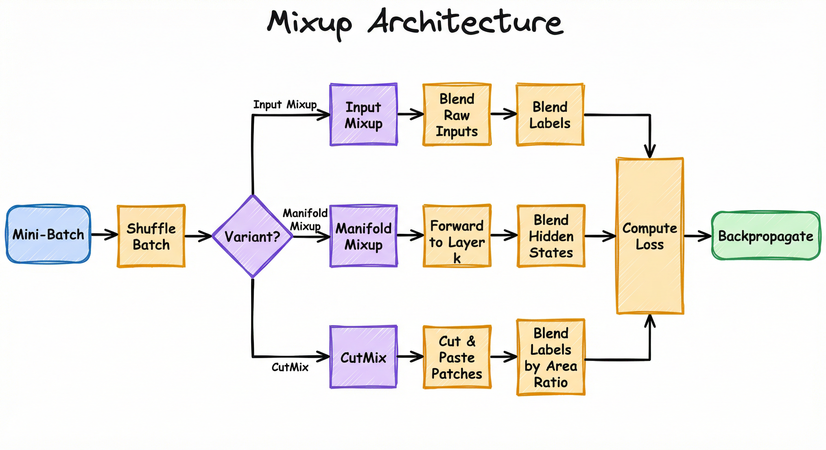
The critical design choice is where to apply the interpolation. Input Mixup operates on raw pixels or features, which is the simplest to implement but produces ghostly blended images. Manifold Mixup applies the blend at a randomly chosen hidden layer, which produces more semantically meaningful interpolations because hidden representations encode higher-level features. CutMix takes a spatial approach, preserving local pixel structures while mixing at the region level.
Key Components
Pair Sampler
Selects pairs of examples for mixing. The standard approach is to shuffle the mini-batch and pair each example with its shuffled counterpart. More advanced strategies include class-aware pairing (mixing across classes) or similarity-aware pairing.
Lambda Sampler
Draws the mixing coefficient from . Typically one is sampled per mini-batch (not per pair) for computational efficiency. Some implementations sample per-pair for finer-grained mixing.
Input Blender
Computes the convex combination for input-level Mixup. For Manifold Mixup, this operates on intermediate feature maps at a randomly selected layer.
Label Blender
Produces soft labels . Requires the loss function to accept soft targets (cross-entropy with soft labels or binary cross-entropy per class).
Loss Adapter
Adapts the loss function to handle soft (non-one-hot) labels. Typically uses nn.CrossEntropyLoss with soft targets or nn.BCEWithLogitsLoss applied per-class, as used in timm's training recipes.
Data Flow
Training Flow: A mini-batch of pairs is loaded from the data loader. The batch is shuffled to create pairs. A single is sampled from . For input Mixup, raw inputs and labels are blended element-wise. For Manifold Mixup, inputs are forwarded through the network to a randomly chosen layer , the hidden states are blended, and the forward pass continues from layer . Labels are blended with the same regardless of variant. The blended batch is passed through the model (or the remaining layers), loss is computed against the soft labels, and gradients are backpropagated normally.
Inference Flow: Standard inference -- no mixing is applied at test time. The model takes a single input and produces a standard prediction. (Some research explores test-time Mixup for uncertainty estimation, but this is not standard practice.)
A directed flow showing a mini-batch being shuffled into pairs, then branching based on the Mixup variant (Input Mixup blends raw inputs, Manifold Mixup blends at a hidden layer, CutMix pastes patches). All variants blend labels with the same lambda. The blended batch flows into loss computation and backpropagation.
How to Implement
Implementing Mixup: Simpler Than You Think
Mixup can be implemented in fewer than 20 lines of code. The core logic is:
- Sample from
- Shuffle the batch to create pairs
- Blend inputs:
- Blend labels:
- Compute cross-entropy loss against soft labels
There are two implementation strategies:
Strategy 1: Collate-level Mixup -- Apply mixing in the DataLoader's collate_fn. This is clean and separates augmentation from training logic, but requires the DataLoader to emit one-hot encoded labels.
Strategy 2: Batch-level Mixup -- Apply mixing inside the training loop after the batch is loaded. This is more flexible and is the approach used by timm and torchvision. It allows dynamic switching between Mixup, CutMix, and no mixing.
For production, Strategy 2 is preferred because it integrates with existing training infrastructure and supports mixing strategy scheduling (e.g., disable Mixup in the last 10 epochs for fine-tuning).
Cost Note: Mixup adds negligible compute overhead -- literally one element-wise multiply and one addition per batch. On an NVIDIA A100 (~\alpha\alpha30 / INR 2,500 on spot instances).
import torch
import numpy as np


def mixup_data(x, y, alpha=0.2):
    """Apply Mixup to a mini-batch.

    Args:
        x: Input tensor of shape (batch_size, ...)
        y: One-hot label tensor of shape (batch_size, num_classes)
        alpha: Beta distribution parameter (0.2 is a safe default)

    Returns:
        mixed_x: Blended inputs
        mixed_y: Blended labels
        lam: The mixing coefficient used
    """
    if alpha > 0:
        lam = np.random.beta(alpha, alpha)
    else:
        lam = 1.0

    batch_size = x.size(0)
    index = torch.randperm(batch_size, device=x.device)

    mixed_x = lam * x + (1 - lam) * x[index]
    mixed_y = lam * y + (1 - lam) * y[index]

    return mixed_x, mixed_y, lam


# Training loop usage
for images, labels in train_loader:
    # Convert to one-hot if needed
    labels_onehot = torch.nn.functional.one_hot(labels, num_classes=10).float()

    mixed_images, mixed_labels, lam = mixup_data(images, labels_onehot, alpha=0.2)

    outputs = model(mixed_images)
    loss = -torch.sum(mixed_labels * torch.log_softmax(outputs, dim=1), dim=1).mean()

    optimizer.zero_grad()
    loss.backward()
    optimizer.step()
This is the canonical Mixup implementation. Key details: (1) We sample a single per batch for efficiency. (2) We shuffle with torch.randperm to create pairs without replacement. (3) The loss must accept soft labels -- standard nn.CrossEntropyLoss with integer labels won't work. We use the manual soft cross-entropy formulation here. In practice, timm uses nn.BCEWithLogitsLoss for better numerical stability.
from timm.data.mixup import Mixup
from timm.loss import SoftTargetCrossEntropy
import torch

# Configure Mixup + CutMix (standard timm recipe)
mixup_fn = Mixup(
    mixup_alpha=0.8,     # Mixup alpha
    cutmix_alpha=1.0,    # CutMix alpha
    prob=1.0,            # Probability of applying either
    switch_prob=0.5,     # Probability of CutMix vs Mixup
    mode='batch',        # One lambda per batch
    num_classes=1000,
)

# Use SoftTargetCrossEntropy for soft labels
criterion = SoftTargetCrossEntropy()

# Training loop
for images, labels in train_loader:
    images, labels = mixup_fn(images, labels)  # labels become soft
    outputs = model(images)
    loss = criterion(outputs, labels)

    optimizer.zero_grad()
    loss.backward()
    optimizer.step()
The timm library provides a production-grade Mixup implementation that supports switching between Mixup and CutMix with configurable probability. The switch_prob=0.5 means each batch has a 50% chance of Mixup and 50% chance of CutMix -- this is the default in modern training recipes like ResNet Strikes Back (Wightman et al., 2021). The SoftTargetCrossEntropy loss handles the soft labels automatically.
import torch
import torch.nn as nn
import numpy as np


class ManifoldMixupModel(nn.Module):
    """ResNet-like model with Manifold Mixup support."""

    def __init__(self, base_model, num_layers=4):
        super().__init__()
        self.layers = nn.ModuleList([
            base_model.layer1,
            base_model.layer2,
            base_model.layer3,
            base_model.layer4,
        ])
        self.stem = nn.Sequential(
            base_model.conv1, base_model.bn1, base_model.relu, base_model.maxpool
        )
        self.avgpool = base_model.avgpool
        self.fc = base_model.fc
        self.num_layers = num_layers

    def forward(self, x, y=None, alpha=0.2, manifold_mixup=True):
        # Choose a random layer to apply Mixup
        if manifold_mixup and self.training and y is not None:
            mix_layer = np.random.randint(0, self.num_layers)
            lam = np.random.beta(alpha, alpha) if alpha > 0 else 1.0
            index = torch.randperm(x.size(0), device=x.device)
        else:
            mix_layer = -1
            lam = 1.0
            index = None

        out = self.stem(x)

        for i, layer in enumerate(self.layers):
            out = layer(out)
            if i == mix_layer:
                # Apply Mixup at this hidden layer
                out = lam * out + (1 - lam) * out[index]

        out = self.avgpool(out)
        out = torch.flatten(out, 1)
        out = self.fc(out)

        if y is not None and index is not None:
            mixed_y = lam * y + (1 - lam) * y[index]
            return out, mixed_y
        return out
Manifold Mixup (Verma et al., 2019) applies the interpolation at a randomly selected hidden layer instead of the input. This produces more semantically meaningful blends because hidden representations encode higher-level features. The key insight: mixing at deeper layers blends semantic concepts (e.g., 'fur texture' + 'wheel shape') rather than raw pixels, producing better regularization. The random layer selection ensures the model learns smooth representations at all levels.
import torch
import torch.nn as nn
import numpy as np
from transformers import AutoModel, AutoTokenizer


class SentenceMixupClassifier(nn.Module):
    """Text classifier with embedding-level Mixup."""

    def __init__(self, model_name='bert-base-uncased', num_classes=4):
        super().__init__()
        self.encoder = AutoModel.from_pretrained(model_name)
        self.classifier = nn.Linear(768, num_classes)
        self.dropout = nn.Dropout(0.1)

    def forward(self, input_ids, attention_mask, labels=None, alpha=0.2):
        # Get word embeddings (before transformer layers)
        embeddings = self.encoder.embeddings(input_ids)

        # Apply Mixup at the embedding level during training
        if self.training and labels is not None and alpha > 0:
            lam = np.random.beta(alpha, alpha)
            batch_size = embeddings.size(0)
            index = torch.randperm(batch_size, device=embeddings.device)

            embeddings = lam * embeddings + (1 - lam) * embeddings[index]
            attention_mask = torch.max(attention_mask, attention_mask[index])

            mixed_labels = lam * labels + (1 - lam) * labels[index]
        else:
            mixed_labels = labels

        # Continue forward pass with mixed embeddings
        outputs = self.encoder(
            inputs_embeds=embeddings,
            attention_mask=attention_mask,
        )
        pooled = outputs.last_hidden_state[:, 0]  # [CLS] token
        logits = self.classifier(self.dropout(pooled))

        return logits, mixed_labels


# Usage
tokenizer = AutoTokenizer.from_pretrained('bert-base-uncased')
model = SentenceMixupClassifier(num_classes=4)

# In training loop:
# logits, mixed_labels = model(input_ids, attention_mask, labels_onehot, alpha=0.2)
# loss = -torch.sum(mixed_labels * torch.log_softmax(logits, dim=1), dim=1).mean()
For NLP, Mixup cannot operate on raw token IDs (discrete integers are not interpolatable). Instead, we apply Mixup at the embedding level -- after tokens are mapped to continuous vectors but before the transformer layers. This approach, explored by Guo et al. (2019), blends the dense representations of two sentences. The attention mask is merged with torch.max to ensure all tokens from both sentences are attended to. This is simpler than CutMix-style span replacement approaches like SSMix but consistently effective across classification tasks.
# timm training config (YAML equivalent)
augmentation:
  mixup_alpha: 0.8        # Beta distribution alpha for Mixup
  cutmix_alpha: 1.0       # Beta distribution alpha for CutMix
  mixup_prob: 1.0         # Probability of applying augmentation
  mixup_switch_prob: 0.5  # Prob of CutMix vs Mixup per batch
  mixup_mode: batch       # 'batch' or 'pair' or 'elem'
  label_smoothing: 0.1    # Additional label smoothing (stacks with Mixup)

training:
  loss: bce               # Use BCE for soft labels
  epochs: 300
  warmup_epochs: 5
  disable_mixup_epochs: 0 # Set > 0 to disable in final epochs
Common Implementation Mistakes
- ●
Using integer labels with standard CrossEntropyLoss: PyTorch's
nn.CrossEntropyLossexpects integer class indices, not soft probability distributions. With Mixup, labels become soft (e.g., [0.7, 0.3]). You must either usenn.BCEWithLogitsLoss, manually compute soft cross-entropy, or usetimm.loss.SoftTargetCrossEntropy. This is the #1 Mixup implementation bug. - ●
Setting alpha too high: With , most blends are near 50-50, producing heavily ghosted images that are hard for the network to learn from. For most tasks, is the safe default. Values above 0.4 rarely help for image classification. I've seen teams waste weeks debugging accuracy drops caused by .
- ●
Applying Mixup at inference time: Mixup is a training-time technique. At test time, use the model normally on unmodified inputs. Some codebases accidentally leave Mixup enabled in eval mode, silently blending test examples and producing nonsensical predictions.
- ●
Mixing within the same class only: Mixup works best when it mixes examples from different classes. Intra-class Mixup still provides some regularization, but the label-smoothing effect vanishes because both labels are identical. The original paper pairs examples randomly, which naturally produces cross-class mixes.
- ●
Forgetting to handle evaluation metrics: During training with Mixup, your training accuracy metric is meaningless because you're comparing predictions to soft labels. Always evaluate on a held-out validation set without Mixup to get accurate performance numbers.
- ●
Not symmetrizing lambda: Some implementations forget to enforce to ensure the first example always has the larger weight. This is a trick from the original paper that prevents the mixed example from being dominated by the shuffled (random) example, improving training stability.
When Should You Use This?
Use When
Training any classification model (image, text, audio, tabular) where you want better generalization with zero architecture changes -- Mixup is the lowest-effort regularizer you can add
Your model is overconfident: predictions cluster near 0.0 and 1.0 instead of reflecting true uncertainty. Mixup's implicit label smoothing directly addresses miscalibration
You need robustness to noisy or corrupted labels. Mixup degrades gracefully under label noise (Zhang et al. showed it tolerates up to 40% label corruption with minimal accuracy loss)
You want improved adversarial robustness without explicit adversarial training (which is 10-50x more expensive). Mixup reduces vulnerability to FGSM and PGD attacks by 10-30%
Your dataset is small or moderately sized (10K-500K examples) and you cannot collect more labeled data. Mixup effectively expands your training distribution
You are using a modern training recipe (e.g., timm, torchvision's modern training) and want to follow established best practices -- Mixup/CutMix is included by default
Avoid When
Your task requires pixel-precise localization (object detection, semantic segmentation, instance segmentation) -- input Mixup blends spatial information, making bounding box and mask labels meaningless. Use CutMix instead, which preserves spatial locality
You are working with ordered or sequential inputs where linear interpolation of raw features is semantically meaningless (e.g., raw text token IDs, categorical tabular features with no ordinal relationship). Apply Mixup in embedding space instead
Your training pipeline uses hard negative mining or contrastive learning where precise pair relationships matter. Mixup disrupts the careful sampling strategy these methods rely on
The number of classes is very large (>10,000) and classes are highly fine-grained. The linear interpolation assumption becomes weaker when nearby classes share subtle distinguishing features -- blending a Labrador with a Golden Retriever doesn't create a meaningful intermediate concept
You are fine-tuning a pre-trained model for only a few epochs (<5). Mixup needs sufficient training time to provide its regularization benefit. For very short fine-tuning, it may hurt convergence
Your model is already well-regularized with dropout, weight decay, and strong data augmentation (e.g., RandAugment + Cutout). Adding Mixup on top provides diminishing returns and may over-regularize, reducing training accuracy without improving validation accuracy
Key Tradeoffs
The Central Tradeoff: Regularization Strength vs. Training Speed
Mixup introduces a tension between regularization strength and training efficiency. Higher values produce stronger regularization (more aggressive blending), but the model needs more epochs to converge because it never sees clean, unblended examples. The original paper trains for 200 epochs on CIFAR with Mixup versus 200 epochs without -- but the Mixup model hasn't fully converged at 200 epochs while the ERM model has. Given 300+ epochs, Mixup pulls further ahead.
| Alpha | Regularization | Convergence Speed | Best For |
|---|---|---|---|
| 0.1 | Light | Fast | Large datasets, short schedules |
| 0.2 | Moderate | Moderate | General purpose (recommended) |
| 0.4 | Strong | Slow | Small datasets, long schedules |
| 1.0 | Very strong | Very slow | Extreme overfitting scenarios |
Mixup vs. CutMix: When to Choose Which
CutMix consistently outperforms Mixup on localization-dependent tasks (object detection, weakly-supervised localization) because it preserves local spatial structure. On pure classification, their performance is similar, with CutMix often having a slight edge on ImageNet (+0.5-1.0%). The modern consensus is to use both together with 50% probability each (the timm default), which outperforms either alone.
Compute Cost: Nearly Free
Mixup adds one element-wise multiplication and one addition per batch -- less than 0.01% of the forward-backward pass cost. The true cost is the extended training schedule needed to fully realize the regularization benefit. On a single NVIDIA A100 GPU, training ResNet-50 on ImageNet for 300 epochs (with Mixup) versus 90 epochs (without) adds approximately $200 (~INR 16,800) in cloud compute. But the accuracy gain is typically 1-2 percentage points, which is well worth it for production models.
Practical Recommendation: Use Mixup + CutMix together with
switch_prob=0.5, , , and train for 300+ epochs. This is the default intimmand consistently delivers best results across architectures.
Alternatives & Comparisons
CutMix cuts a rectangular patch from one image and pastes it onto another, mixing labels proportionally to the patch area. It preserves local pixel structure that Mixup destroys (Mixup creates ghostly overlays), making CutMix superior for tasks requiring spatial awareness like object detection and weakly-supervised localization. On pure classification, CutMix has a slight edge (+0.5-1.0% on ImageNet). In practice, the best approach is to use both with 50% probability each per batch.
Traditional image augmentations (rotation, flip, color jitter, RandAugment) transform single images while preserving labels. They encode domain-specific invariances (rotation invariance, color invariance) that Mixup does not. Mixup is complementary to these techniques -- it provides inter-sample regularization while traditional augmentations provide intra-sample variation. Modern training recipes use both together.
Text augmentation techniques like back-translation, synonym replacement, and random insertion operate on discrete tokens and preserve semantic meaning. For NLP, these are often more natural than Mixup because they produce readable text. However, embedding-level Mixup can be combined with text augmentations for additional regularization, especially in low-resource settings.
SMOTE also interpolates between examples but specifically targets minority class samples for class imbalance problems. Unlike Mixup, SMOTE generates synthetic examples offline (before training) and focuses on rebalancing class distributions rather than regularization. Mixup operates on-the-fly during training and mixes across classes, serving a fundamentally different purpose. For class-imbalanced datasets, combining class-weighted Mixup with SMOTE-like strategies can be effective.
Pros, Cons & Tradeoffs
Advantages
Near-zero computational overhead: One element-wise multiply and one addition per batch -- less than 0.01% of forward-backward pass cost. The cheapest regularizer you can add to any training pipeline.
Domain-agnostic: Works on images, text (in embedding space), audio, tabular data, and multi-modal inputs. No domain-specific transformation design required -- just blend and go.
Improved calibration: Models trained with Mixup produce better-calibrated confidence scores. On CIFAR-100, Expected Calibration Error (ECE) drops by 30-50% compared to ERM. This matters enormously for safety-critical applications.
Robust to label noise: Mixup tolerates up to 40% label corruption with minimal accuracy loss (Zhang et al., 2018). In messy real-world datasets with crowd-sourced labels -- common in Indian data annotation pipelines -- this resilience is invaluable.
Improved adversarial robustness: Top-1 error under FGSM adversarial attacks improves by 10-30% without any explicit adversarial training. This is free robustness.
Implicit label smoothing: Naturally prevents overconfident predictions, reducing the need for separate label smoothing hyperparameters. One technique, two benefits.
Trivial to implement: 5-10 lines of code in PyTorch. Available out-of-the-box in
timm,torchvision, andkeras. No reason not to try it.
Disadvantages
Destroys spatial locality: Blending two images pixel-wise creates ghostly overlays where local structures from both images interfere. For tasks requiring localization (detection, segmentation), this is harmful. CutMix addresses this limitation.
Requires soft-label-compatible loss function: Standard
nn.CrossEntropyLosswith integer labels won't work. You need to switch to soft cross-entropy or BCE loss -- a small but non-obvious implementation change that trips up many practitioners.Slower convergence: The model needs more training epochs (typically 1.5-2x) to fully benefit from Mixup because it never sees clean examples. For teams with tight compute budgets (~INR 50,000/month GPU allocation), the extended schedule adds cost.
Alpha sensitivity: Performance is sensitive to the hyperparameter. Too low () and Mixup has no effect; too high () and training degrades. A hyperparameter sweep over 3-5 values is usually needed.
Semantic assumption can fail: Linear interpolation in pixel space doesn't always produce semantically meaningful blends. A 50-50 blend of a cat and a car is not a meaningful concept -- it's just a confusing ghost image. The model must learn to ignore this noise.
Training metrics become unreliable: Training accuracy and loss against mixed labels are not directly comparable to validation metrics on clean data. This can confuse monitoring dashboards and make debugging harder.
Less effective for fine-grained tasks: When classes are visually very similar (e.g., bird species, car models), blending examples from nearby classes can produce ambiguous training signals that hurt more than they help.
Failure Modes & Debugging
Alpha too high: training collapse
Cause
Setting concentrates the Beta distribution near , meaning every training example is a near-equal blend of two unrelated images. The model receives mostly ambiguous, unnatural inputs and cannot learn discriminative features.
Symptoms
Training loss decreases very slowly or plateaus at a high value. Validation accuracy stagnates 5-15% below the ERM baseline even after extended training. The model predicts near-uniform probabilities across classes, essentially having learned nothing discriminative.
Mitigation
Start with (the original paper's recommendation). Only increase to for very small datasets where stronger regularization is needed. Never exceed without extensive ablation. If validation accuracy is below the ERM baseline after 50% of training epochs, reduce immediately.
Soft label loss mismatch
Cause
Using nn.CrossEntropyLoss(reduction='mean') with integer target labels while feeding Mixup-blended inputs. The loss function expects integer class indices but receives mixed inputs, so it optimizes against the wrong label -- the original unblended label of the first example in the pair.
Symptoms
Training appears normal (loss decreases, accuracy improves) but the model underperforms the ERM baseline. The Mixup augmentation is effectively ignored because the labels are never blended. This is a silent failure -- no error is raised, the model just trains suboptimally.
Mitigation
Always verify that labels are one-hot encoded and blended with the same . Use timm.loss.SoftTargetCrossEntropy or manually compute soft cross-entropy: loss = -torch.sum(soft_labels * log_softmax(logits), dim=1).mean(). Add an assertion that labels sum to 1.0 and are not one-hot during the first few batches.
Manifold Mixup at the wrong layer
Cause
Applying Manifold Mixup consistently at a very deep layer (near the output) where representations are already near-linear. The regularization effect is minimal because the model has already separated classes at this point.
Symptoms
No improvement over input-level Mixup despite the additional implementation complexity. The training dynamics look identical to input Mixup, suggesting the hidden-layer mixing is not providing additional benefit.
Mitigation
Randomly sample the mixing layer during training (the approach recommended by Verma et al., 2019). Include the input layer (layer 0) in the sampling pool. The randomization forces smooth representations at all levels of the network. If a specific layer consistently underperforms, exclude it from the sampling set.
Mixup hurting localization tasks
Cause
Applying input-level Mixup to object detection or segmentation models. The pixel-level blending destroys spatial structure, making bounding box regression and mask prediction targets meaningless for the blended regions.
Symptoms
Object detection mAP drops by 2-5% compared to the no-Mixup baseline. The model produces diffuse, poorly localized bounding boxes. Segmentation masks become blurry at object boundaries.
Mitigation
For detection and segmentation, use CutMix instead of Mixup. CutMix preserves local pixel structure within the pasted patch. If Mixup must be used, apply Manifold Mixup at a feature map level after the backbone, where spatial resolution is already reduced (e.g., at 7x7 feature maps).
NLP token-level Mixup producing garbage
Cause
Attempting to apply Mixup directly to raw token IDs (integers). Linear interpolation between token IDs 5034 and 2817 produces 3925.5 -- a non-existent token. The model receives corrupt, meaningless inputs.
Symptoms
Complete training failure. Loss does not decrease. The model outputs random predictions. If the framework silently rounds the interpolated IDs, the model trains on completely wrong tokens.
Mitigation
Never apply Mixup to discrete inputs (token IDs, categorical features). For NLP, apply Mixup at the embedding level (after the embedding lookup layer) or at hidden-state levels. For tabular data with categorical features, apply Mixup only to the continuous features or after embedding the categoricals.
Evaluation metric confusion
Cause
Reporting training accuracy computed against Mixup soft labels as if it were standard accuracy. Since Mixup labels are soft (e.g., [0.7, 0.3]), the argmax prediction of a well-trained model may match the dominant class but the soft cross-entropy loss will still be high.
Symptoms
Training loss appears much higher than expected. Training accuracy appears lower than the validation accuracy throughout training, which is confusing for monitoring. Teams may incorrectly conclude the model is underfitting.
Mitigation
Always evaluate on a clean validation set without Mixup. Log training loss and validation loss separately. If using training accuracy for monitoring, compute it against the hard (argmax) label of the dominant class in the mix, not the soft label.
Placement in an ML System
Where Mixup Fits in the ML Pipeline
Mixup sits squarely in the training data augmentation stage. It operates between the data loader (which produces clean mini-batches) and the model's forward pass (which consumes augmented mini-batches). In a typical PyTorch training loop, Mixup is applied after the batch is loaded and before it enters the model.
In production ML systems, Mixup is configured as part of the training recipe alongside other augmentations (RandAugment, Cutout, CutMix) and regularizers (dropout, weight decay, label smoothing, stochastic depth). The key design decision is how these components interact -- for example, timm applies RandAugment first (per-image), then Mixup/CutMix (per-batch), then label smoothing (per-label).
At serving time, the Mixup-trained model is deployed exactly like any other model. There are no special inference requirements, no additional latency, and no architectural modifications. This makes Mixup ideal for training-time improvements that don't add inference cost -- a highly valued property in latency-sensitive production systems like Flipkart's product recommendations or Swiggy's ETA predictions.
Key Insight: Mixup is a training-only component. It improves the model without adding any inference-time overhead. This makes it one of the few techniques that is purely beneficial in cost-constrained production environments.
Pipeline Stage
Training / Data Augmentation
Upstream
- Training Data Pipeline
- Data Loader
- Feature Store
Downstream
- Model Training Loop
- Loss Function
- Model Registry
Scaling Bottlenecks
Mixup itself has virtually no scaling bottleneck -- it's a single element-wise operation that runs in microseconds. The bottleneck is the extended training schedule it requires. On a 100-GPU cluster training a large vision transformer, adding Mixup doesn't slow down individual steps, but increasing the schedule from 90 to 300 epochs multiplies total compute by 3.3x.
For distributed training, Mixup can be applied independently per GPU (each GPU shuffles its local batch and blends locally). There is no cross-GPU communication overhead. However, if you want to mix examples across GPUs (for greater diversity), you need an all_gather operation which adds inter-node latency. In practice, local-batch Mixup works well enough.
At inference time, there is zero overhead because Mixup is disabled. The trained model is a standard neural network with no architectural modifications.
Some concrete numbers: training ResNet-50 on ImageNet with Mixup on 8x A100 GPUs takes approximately 30 hours for 300 epochs (~145 / INR 12,000.
Production Case Studies
Mixup was originally developed at Facebook AI Research (now Meta) and MIT. The team released the reference implementation alongside the ICLR 2018 paper. Meta subsequently incorporated Mixup into their internal training pipelines for image classification and representation learning. The timm library, widely used for training production vision models, adopted Mixup as a default augmentation in its modern training recipes.
On CIFAR-10, Mixup reduced test error from 4.2% (ERM baseline) to 3.6% -- a 14% relative improvement. On ImageNet with ResNet-50, Mixup improved top-1 accuracy from 76.3% to 77.2%. These improvements have been reproduced across thousands of projects and are now considered standard baseline results.
Google and the PyTorch team's modern training recipes for torchvision include Mixup and CutMix as standard components. The 'ResNet Strikes Back' training procedure (Wightman et al., 2021) showed that ResNet-50 -- an architecture from 2015 -- could achieve 80.4% top-1 accuracy on ImageNet when trained with modern augmentation recipes including Mixup/CutMix, closing the gap with newer architectures like EfficientNet and Vision Transformers.
ResNet-50 accuracy improved from 76.1% (original 2015 recipe) to 80.4% (modern recipe with Mixup/CutMix, RandAugment, and label smoothing). This +4.3 percentage point improvement came entirely from training recipe changes with zero architecture modifications.
Multiple medical imaging research groups have adopted Mixup for training diagnostic classifiers where labeled data is scarce and expensive. Studies on COVID-19 CT classification, thyroid cancer whole-slide image analysis, and psychosis prediction from fMRI data showed consistent improvements when Mixup was added to the training pipeline. This is particularly valuable in India where medical AI startups often face data scarcity due to privacy regulations and limited hospital partnerships.
Mixup improved classification accuracy by 2-5 percentage points across multiple medical imaging tasks. On COVID-19 CT classification, Mixup combined with attention mechanisms achieved state-of-the-art accuracy on the COVID-CT benchmark. For thyroid cancer diagnosis from whole-slide images, MixUp-MIL (Mixup for Multiple Instance Learning) consistently increased accuracy.
Clova AI, the ML research arm of Naver (South Korea's largest search engine), developed CutMix as a spatial alternative to Mixup after identifying that Mixup's pixel blending hurts localization performance. Their research showed that combining CutMix with Mixup (switching between the two with 50% probability per batch) outperformed either technique alone. This combined approach became the standard in timm and torchvision.
CutMix achieved 21.40% top-1 error on ImageNet with ResNet-50, outperforming Mixup (22.58%) by 1.18 percentage points. On weakly-supervised localization (CUB-200), CutMix outperformed Mixup by +5.51% in localization accuracy. The Mixup+CutMix combination is now the de facto standard.
Tooling & Ecosystem
The timm library provides a production-grade Mixup class that supports Mixup, CutMix, and their combination with configurable probabilities, alpha values, and application modes (batch, pair, elem). Used as the default augmentation in timm's training scripts, which produce state-of-the-art image classification results. Includes SoftTargetCrossEntropy loss.
PyTorch's official torchvision library includes v2.MixUp and v2.CutMix transforms as first-class citizens. Integrates with the torchvision transforms pipeline and supports the modern torch.utils.data.DataLoader collate function pattern.
While primarily known for geometric and photometric augmentations, Albumentations provides a composable pipeline where Mixup-style augmentations can be integrated. The MixUp transform is available via community contributions. Widely used in Kaggle competitions and Indian ML startups for its fast, OpenCV-backed transforms.
A comprehensive benchmarking framework for mix-based augmentation methods. Implements 20+ Mixup variants (Vanilla Mixup, CutMix, SaliencyMix, FMix, PuzzleMix, ResizeMix, etc.) with standardized benchmarks on CIFAR-10/100 and ImageNet. Essential for comparing Mixup variants under controlled conditions.
Keras provides MixUp and CutMix as preprocessing layers that can be added to the data pipeline. TensorFlow users can also implement Mixup via tf.data map operations. The Keras implementation handles label mixing automatically.
NVIDIA's Data Loading Library provides GPU-accelerated data augmentation pipelines. While Mixup isn't a built-in operation, DALI's composable pipeline makes it easy to implement Mixup as a custom operation that runs on GPU, eliminating CPU-GPU transfer bottlenecks for large-scale training jobs.
Research & References
Zhang, Cisse, Dauphin & Lopez-Paz (2018)ICLR 2018
The foundational Mixup paper. Proposed training on convex combinations of input pairs and their labels, demonstrating improvements on CIFAR-10/100, ImageNet, and speech commands. Showed Mixup reduces memorization, improves adversarial robustness, and stabilizes GAN training. Over 7,000 citations.
Verma, Lamb, Beckham, Najafi, Mitliagkas, Lopez-Paz & Bengio (2019)ICML 2019
Extended Mixup to hidden layers, showing that interpolating intermediate representations produces better-calibrated models with flatter class representations (fewer directions of variance). Proved theoretical conditions under which Manifold Mixup avoids underfitting.
Yun, Han, Oh, Chun, Choe & Yoo (2019)ICCV 2019
Proposed replacing rectangular regions (instead of pixel-level blending) to preserve spatial structure. Achieved 21.40% top-1 error on ImageNet with ResNet-50, outperforming Mixup by 1.18%. Now used alongside Mixup as a standard augmentation component.
Carratino, Cisse, Cevher & Pontil (2022)Journal of Machine Learning Research
Provided the first rigorous theoretical analysis of Mixup, showing it induces both label smoothing and Lipschitz regularization. Demonstrated that at test time, applying a data transformation (reflecting the Mixup distribution) improves accuracy and calibration.
Guo, Mao & Zhang (2019)arXiv preprint
Systematically studied Mixup for NLP, proposing wordMixup (interpolation at word embedding level) and senMixup (interpolation at sentence embedding level). Both variants improved text classification accuracy, with senMixup generally outperforming wordMixup.
Zou, Cao, Li & Gu (2023)ICML 2023
Provided theoretical analysis explaining why Mixup learns better features than ERM, showing that Mixup learns all relevant features while ERM may only learn the most prominent ones. This explains Mixup's superior out-of-distribution generalization.
Thulasidasan, Chennupati, Bilmes, Bhatt & Philipose (2019)NeurIPS 2019
Demonstrated that Mixup-trained networks are significantly better calibrated than ERM-trained networks. Expected Calibration Error (ECE) improved by 30-50% on CIFAR-100. Also showed Mixup improves predictive uncertainty estimates under distribution shift.
Interview & Evaluation Perspective
Common Interview Questions
- ●
What is Mixup and how does it differ from traditional data augmentation?
- ●
Explain the role of the Beta distribution in Mixup. What happens when you change alpha?
- ●
How does Mixup act as a regularizer? What is its connection to label smoothing?
- ●
When would you use Mixup vs. CutMix vs. traditional augmentation?
- ●
Can Mixup be applied to NLP or tabular data? What are the challenges?
- ●
How does Mixup improve adversarial robustness without explicit adversarial training?
- ●
What is Manifold Mixup and why might it be better than input-level Mixup?
Key Points to Mention
- ●
Mixup trains on convex combinations of pairs: , , where . The single hyperparameter controls mixing strength.
- ●
Mixup provides three forms of regularization simultaneously: (1) data augmentation by creating virtual examples, (2) implicit label smoothing by producing soft targets, and (3) Lipschitz regularization by encouraging linear behavior between training points.
- ●
The connection to Vicinal Risk Minimization (VRM): ERM trains on point estimates, Mixup trains on the vicinity between points, approximating the continuous data distribution.
- ●
CutMix preserves spatial locality that Mixup destroys -- critical for localization tasks. Modern recipes use both with 50% probability each (the timm default).
- ●
For NLP, Mixup must be applied in embedding or hidden-state space (never on raw token IDs). SenMixup and wordMixup are the two main strategies.
- ●
Alpha should be small (0.2-0.4 for most tasks). means uniform mixing which is too aggressive; degenerates to no mixing.
Pitfalls to Avoid
- ●
Saying Mixup only works for images -- it's domain-agnostic and works on any continuous feature representation (images, embeddings, audio spectrograms, tabular features).
- ●
Forgetting the loss function requirement: standard CrossEntropyLoss with integer labels doesn't work with Mixup. You need a soft-label-compatible loss.
- ●
Claiming Mixup creates 'more data' in the traditional sense. It doesn't increase your dataset size; it changes the training distribution by sampling virtual examples on-the-fly.
- ●
Not mentioning the convergence tradeoff: Mixup needs more training epochs (1.5-2x) to fully realize its benefit. Applying it with a short schedule can actually hurt.
- ●
Ignoring the connection to calibration and uncertainty: this is a key selling point for production systems and safety-critical applications.
Senior-Level Expectation
A senior candidate should discuss Mixup as part of a broader training recipe, not in isolation. They should know the modern timm defaults (Mixup , CutMix , switch probability 0.5, BCE loss) and explain why this combination works. They should articulate the theoretical foundations -- VRM, label smoothing connection, Lipschitz regularization -- and connect these to practical outcomes (calibration, adversarial robustness). They should identify when Mixup fails (localization tasks, discrete inputs, very short fine-tuning schedules) and propose alternatives (CutMix, Manifold Mixup, domain-specific augmentations). For production systems, they should discuss how Mixup fits into the training pipeline (training-only, zero inference cost), hyperparameter selection strategy ( sweep with validation), and monitoring (separate training and validation metrics). Bonus points for mentioning recent theory (Zou et al. 2023 on feature learning benefits) and awareness of advanced variants (PuzzleMix, SaliencyMix, Co-Mixup).
Summary
Mixup is a training-time data augmentation and regularization technique that constructs virtual training examples by taking convex combinations of pairs of inputs and their labels. Proposed by Zhang et al. at ICLR 2018, it's one of the most impactful yet simplest techniques in modern deep learning: blend , blend , where , and train normally. Five lines of code, zero architectural changes, negligible compute overhead.
The power of Mixup lies in its triple regularization effect: it generates virtual training examples (data augmentation), produces soft targets (implicit label smoothing), and enforces linear behavior between training points (Lipschitz regularization). These mechanisms improve generalization, calibration, and adversarial robustness simultaneously. The technique is domain-agnostic -- it works on images, embeddings, audio spectrograms, and tabular features -- and has been extended to hidden layers (Manifold Mixup), spatial regions (CutMix), and NLP (SentMixup). Modern training recipes in timm and torchvision use Mixup and CutMix together as default augmentations, achieving state-of-the-art results on ImageNet without architectural innovation.
For production ML systems, Mixup is uniquely attractive because it improves the model at training time without adding any inference-time cost. The trained model is a standard neural network with no special serving requirements. The main costs are (1) a hyperparameter sweep over values and (2) an extended training schedule to fully realize the regularization benefit. For most teams, the recommended starting point is with Mixup and CutMix combined at 50% probability each -- the same recipe that pushes ResNet-50 from 76.1% to 80.4% on ImageNet.