Image Augmentation in Machine Learning
Let's talk about one of the most powerful yet underappreciated techniques in computer vision: image augmentation. This is the practice of artificially expanding your training dataset by applying transformations — rotations, flips, crops, color shifts — to existing images, creating new variations that help models generalize better.
The insight is deceptively simple: if your model has only seen cats photographed from the left side in bright daylight, it will struggle with cats facing right in dim lighting. Image augmentation systematically exposes the model to these variations during training, teaching it to recognize the underlying object regardless of superficial differences.
But here's what most tutorials won't tell you: augmentation is not a free lunch. Apply the wrong transformations, and you can actually hurt model performance. Flip medical X-rays vertically when anatomical orientation matters? You've just poisoned your training data. Rotate road signs by 180 degrees in an autonomous driving dataset? You're training the model to hallucinate upside-down stop signs.
Today, image augmentation sits at the heart of every production computer vision pipeline — from Google Photos' object recognition to Tesla's autopilot perception systems. The field has evolved from manual specification of transformations to automated augmentation strategies like AutoAugment, RandAugment, and TrivialAugment that search for optimal policies. At inference time, test-time augmentation (TTA) squeezes out additional accuracy by ensembling predictions over multiple augmented views of the same image.
This guide will teach you not just how to augment images, but when to augment, which transformations to apply, and — critically — when augmentation will hurt more than it helps.
Concept Snapshot
- What It Is
- A data augmentation technique that applies label-preserving transformations to training images, creating synthetic variations that improve model generalization and robustness without collecting additional labeled data.
- Category
- Data Generation
- Complexity
- Beginner
- Inputs / Outputs
- Inputs: original images with labels. Outputs: augmented images (rotated, flipped, cropped, color-shifted variants) with the same labels, effectively multiplying dataset size.
- System Placement
- Applied during the training data preprocessing pipeline, immediately before feeding images to the model. Can also be applied at inference time (test-time augmentation) for improved accuracy.
- Also Known As
- data augmentation, image transformation, synthetic data generation, training data augmentation, TTA (test-time augmentation)
- Typical Users
- Computer vision engineers, ML researchers, Deep learning practitioners, Data scientists, Model trainers
- Prerequisites
- Basic understanding of CNNs, Familiarity with image data formats, Overfitting vs generalization concepts
- Key Terms
- geometric transformsphotometric transformsAutoAugmentRandAugmentTrivialAugmenttest-time augmentationmixupcutmixrandom erasingcolor jitteringlabel-preserving
Why This Concept Exists
The Data Hunger Problem
Deep learning models are notoriously data-hungry. A ResNet-50 trained on ImageNet sees 1.28 million labeled images — and that's considered a moderately-sized dataset by modern standards. State-of-the-art vision transformers often train on billions of images.
But here's the catch: labeled data is expensive. Collecting, annotating, and curating a dataset of 100,000 medical images might cost 1,000,000 (roughly ₹4.2-8.4 crore) when you factor in expert radiologist time. For specialized domains — satellite imagery analysis, industrial defect detection, rare disease diagnosis — you might only have a few thousand labeled examples.
Without augmentation, your model will memorize the training set and fail to generalize.
The Geometric Invariance Gap
Natural images exhibit geometric invariances that raw pixel data doesn't capture. A cat rotated 15 degrees is still a cat. A car flipped horizontally is still a car (unless it's a right-hand-drive market and steering wheel position matters for detection). A face zoomed in by 20% is still the same face.
Convolutional neural networks learn translation invariance through their architecture, but they don't automatically learn rotation invariance, scale invariance, or invariance to photometric changes. Image augmentation explicitly encodes these invariances into the training process.
The Regularization Effect
Even when you have enough data, augmentation acts as a powerful regularizer. By showing the model slightly different versions of the same image in each epoch, you prevent it from memorizing exact pixel patterns. This is particularly critical when training large models prone to overfitting.
Research shows that for ImageNet classification, even with 1.28 million images, aggressive augmentation improves top-1 accuracy by 1-3 percentage points. That might sound small, but in competitive benchmarks, 1% is the difference between state-of-the-art and also-ran.
The Real-World Distribution Shift
Your training data rarely matches the distribution of real-world deployment. Training images might all be high-resolution, well-lit, centered crops. But in production, your model will see low-resolution thumbnails, poorly lit scenes, and off-center objects.
Augmentation simulates deployment conditions during training, making models more robust to distribution shift. This is why autonomous vehicle perception models augment with fog, rain, lens flare, and motion blur — to prepare for adverse weather conditions they'll encounter on real roads.
Key Takeaway: Image augmentation exists because collecting infinite labeled data is impossible, and models need to learn invariances and robustness that raw data alone cannot provide. It's the closest thing we have to a free performance boost.
Core Intuition & Mental Model
The Core Guarantee
Here's the fundamental promise of image augmentation: if a transformation doesn't change the semantic label of an image, applying that transformation during training will improve generalization without biasing the model toward incorrect predictions.
Let me unpack that. A label-preserving transformation is one where a human annotator would assign the same label to both the original and transformed image. Rotating a cat photo by 10 degrees? Still a cat. Flipping it horizontally? Still a cat. Cranking up brightness by 30%? Still a cat.
But flip a "7" digit upside-down in MNIST, and it might look like a "1". That's a label-violating transformation — and applying it will actively harm your model.
The Augmentation Recipe: Mix, Don't Replace
A common misconception: augmentation replaces your original dataset. Wrong. Augmentation expands it. In each training epoch, you typically:
- Start with an original image
- Apply a random subset of transformations (the "augmentation policy")
- Feed the augmented image to the model
- Repeat with different random transformations in the next epoch
This means the model sees the same base image in different forms across epochs, learning to extract features invariant to the transformations.
Why Random Matters
You might ask: why apply transformations randomly each epoch instead of pre-generating all augmented versions upfront?
Because randomness acts as a regularizer. If you pre-generate 10 augmented versions of each image, the model will eventually memorize all 10. But if you randomly sample transformations on-the-fly, the model sees a nearly infinite variety — a cat rotated by 7° in epoch 1, 14° in epoch 2, 3° in epoch 3, and so on.
The Label-Preserving Boundary
The art of augmentation is identifying the label-preserving boundary for your specific task:
- Image classification: You can be aggressive. Flips, rotations, crops, color shifts — as long as a human can still identify the object, you're safe.
- Object detection: More careful. Transformations must preserve bounding box relationships. Heavy crops might cut out objects entirely.
- Semantic segmentation: Very careful. Pixel-level labels must be transformed alongside the image. A rotation requires rotating the segmentation mask too.
- Medical imaging: Extremely careful. Anatomical orientation often matters. Horizontal flips might be fine; vertical flips almost never are.
Mental Model: Think of augmentation as showing your model the same scene under different lighting, angles, and zoom levels — all the variations it might encounter in the real world — without changing what the scene depicts. The model learns to ignore superficial differences and focus on the underlying semantic content.
Technical Foundations
The Math (Built Up from First Principles)
Intuition First: You have a dataset of images and labels . Augmentation applies transformations to images while keeping labels unchanged, creating a larger effective dataset .
Formally: Let be a set of transformation functions that map images to (potentially different-sized) images. An augmentation policy selects transformations from and composes them.
For a single image with label , augmentation generates:
where are transformations sampled from the policy. The augmented pair is — crucially, the label remains unchanged.
The augmented dataset becomes:
Common Transformation Families
Geometric Transformations (preserve spatial structure with modification):
- Rotation: rotates image by angle
- Horizontal/Vertical Flip:
- Random Crop: extracts region of size starting at
- Affine Transforms: applies affine matrix and translation
Photometric Transformations (preserve spatial structure, modify appearance):
- Brightness:
- Contrast:
- Color Jitter: Random perturbations to HSV channels
Occlusion/Erasing:
- Random Erasing: sets random region to random values
- Cutout: Similar, but fills region with zeros or mean pixel value
Mixing Augmentations
Modern techniques blend multiple images:
Mixup: Given two images and :
where for some hyperparameter (typically 0.2-0.4).
CutMix: Cuts a rectangular region from and pastes it into , mixing labels proportionally to the area:
where is the ratio of the cut region area to total image area.
AutoAugment and Learned Policies
Instead of manually choosing transformations, AutoAugment formulates augmentation policy search as a reinforcement learning problem:
- Policy: A set of sub-policies, each containing operations (typically )
- Operation: where is a transformation type, is probability of application, is magnitude
- Search: Use RL to find the policy that maximizes validation accuracy
RandAugment simplifies this: instead of learning probabilities and magnitudes per operation, it uses two global hyperparameters:
- : number of operations to apply in sequence
- : global magnitude for all operations (distortion strength)
This reduces the search space from (AutoAugment) to just configurations.
TrivialAugment goes even simpler: for each image, randomly select one transformation and one magnitude. No hyperparameters to tune. Surprisingly, this often matches or exceeds RandAugment's performance.
Warning: The label-preserving assumption is critical. Formally, we require that for all transformations : If this doesn't hold, augmentation introduces label noise and degrades performance.
Internal Architecture
Image augmentation is typically implemented as a preprocessing pipeline that transforms images on-the-fly during training. The pipeline consists of four stages: transformation sampling (selecting which augmentations to apply based on the policy), transformation application (executing geometric and photometric operations), batch assembly (collating augmented images into mini-batches), and optional normalization. At inference time, test-time augmentation (TTA) applies the same pipeline to create multiple views of test images, ensembling predictions for higher accuracy.
Key Components
Transformation Sampler
Selects which transformations to apply based on the augmentation policy (random, AutoAugment, RandAugment, etc.). Samples transformation types, probabilities, and magnitudes.
Geometric Transform Engine
Applies spatial transformations like rotation, flipping, cropping, affine warping, and perspective shifts. Handles interpolation and boundary conditions.
Photometric Transform Engine
Applies color-space transformations including brightness, contrast, saturation, hue adjustments, color jittering, and histogram equalization.
Mixing/Erasing Module
Implements advanced augmentations like Mixup (blending two images), CutMix (cutting and pasting regions), Cutout/Random Erasing (occluding random patches).
Batch Assembly & Normalization
Collates augmented images into mini-batches, applies channel normalization (mean subtraction, std division), and handles variable image sizes through padding or resizing.
Test-Time Augmentation (TTA)
At inference, generates multiple augmented views of each test image, runs model inference on all views, and ensembles predictions (averaging logits or probabilities) for final output.
Data Flow
Here's the typical flow:
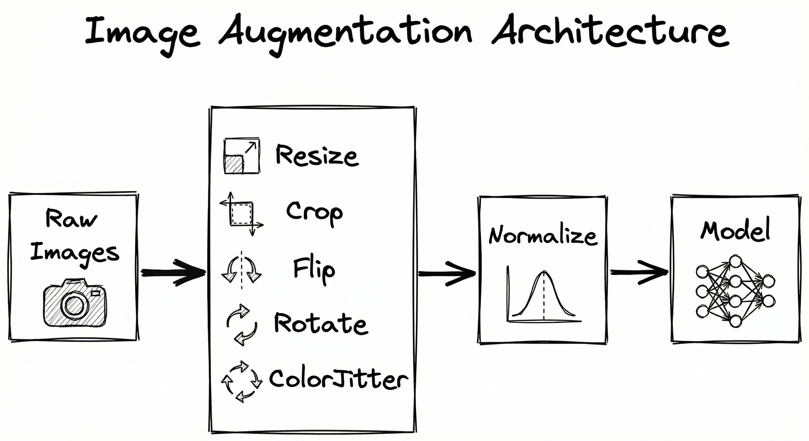
Training Path: Raw image loaded → Transformation sampler selects policy (e.g., RandAugment with N=2, M=10) → Geometric transforms applied (random crop, horizontal flip) → Photometric transforms applied (color jitter, brightness adjustment) → Optional mixing (Mixup with another image) → Batch assembly → Normalization → Fed to model.
Inference Path (Standard): Test image → Resize to fixed size → Normalization → Model inference → Prediction.
Inference Path (with TTA): Test image → Generate K augmented views (original, flip, rotations, crops) → Run model on all K views → Average predictions → Final prediction. This typically increases inference time by K× but improves accuracy by 0.5-2%.
A directed flow showing raw images branching through geometric, photometric, and mixing transforms in parallel, then converging to batch assembly and model training. A separate TTA path shows test images generating multiple augmented views that flow through model inference to ensembled predictions.
How to Implement
Three Layers of Implementation Sophistication
Layer 1: Basic transforms — Use library defaults (torchvision, albumentations) with standard geometric and photometric augmentations. Good for prototyping and small-to-medium datasets.
Layer 2: Automated policies — Implement RandAugment or TrivialAugment for automatic selection of transformations and magnitudes. Minimal hyperparameter tuning required.
Layer 3: Custom search — Run AutoAugment-style policy search optimized for your specific dataset and task. Expensive but yields best results for production systems.
For most practitioners, Layer 2 hits the sweet spot: better than manual tuning, less expensive than full search.
Library Ecosystem
The Python ecosystem offers several mature libraries:
- Albumentations: Fast, flexible, supports detection/segmentation with bounding box transforms. Best for production pipelines.
- torchvision.transforms.v2: PyTorch's official library, tight integration with dataloaders. Best for pure PyTorch workflows.
- imgaug: Versatile, multi-core support, slightly slower than Albumentations. Maintenance has slowed (last update 2023).
- Keras/TensorFlow tf.image: Built-in augmentation layers. Best for Keras-centric stacks.
Cost Note: All these libraries are open-source and free. Cloud compute costs dominate: training with aggressive augmentation on a 100K-image dataset might require an extra 20-30% GPU time compared to no augmentation, translating to roughly $50-100/month (~₹4,200-8,400/month) on cloud GPUs.
import albumentations as A
from albumentations.pytorch import ToTensorV2
import cv2

# Define augmentation pipeline
transform = A.Compose([
    A.HorizontalFlip(p=0.5),
    A.RandomRotate90(p=0.5),
    A.ShiftScaleRotate(shift_limit=0.0625, scale_limit=0.1, rotate_limit=15, p=0.5),
    A.RandomBrightnessContrast(brightness_limit=0.2, contrast_limit=0.2, p=0.5),
    A.ColorJitter(brightness=0.2, contrast=0.2, saturation=0.2, hue=0.1, p=0.5),
    A.GaussianBlur(blur_limit=(3, 7), p=0.3),
    A.Normalize(mean=[0.485, 0.456, 0.406], std=[0.229, 0.224, 0.225]),
    ToTensorV2(),
])

# Apply to image
image = cv2.imread('cat.jpg')
image = cv2.cvtColor(image, cv2.COLOR_BGR2RGB)
augmented = transform(image=image)
augmented_image = augmented['image']  # Normalized PyTorch tensor
Albumentations provides a composable pipeline where each transformation has a probability 'p' of being applied. This example combines geometric transforms (flip, rotate, shift-scale-rotate) with photometric transforms (brightness-contrast, color jitter, blur). The pipeline is applied on-the-fly in the dataset getitem method, ensuring random variations each epoch. Albumentations is significantly faster than torchvision for complex pipelines (2-3x speedup in benchmarks).
import torch
from torchvision import transforms
from torchvision.transforms import autoaugment

# RandAugment with N=2 operations, magnitude M=9
transform = transforms.Compose([
    transforms.RandomResizedCrop(224),
    transforms.RandAugment(num_ops=2, magnitude=9),
    transforms.ToTensor(),
    transforms.Normalize(mean=[0.485, 0.456, 0.406], std=[0.229, 0.224, 0.225]),
])

# Apply to PIL image
from PIL import Image
image = Image.open('dog.jpg')
augmented_tensor = transform(image)

# For TrivialAugment (even simpler, no hyperparameters)
trivial_transform = transforms.Compose([
    transforms.RandomResizedCrop(224),
    transforms.TrivialAugmentWide(),  # Randomly picks 1 operation per image
    transforms.ToTensor(),
    transforms.Normalize(mean=[0.485, 0.456, 0.406], std=[0.229, 0.224, 0.225]),
])
RandAugment drastically simplifies augmentation policy search by reducing it to two hyperparameters: num_ops (N) controls how many operations to chain, and magnitude (M) controls the distortion strength (0-30 scale, where 10 is moderate). TrivialAugmentWide is even simpler: it randomly selects exactly one transformation per image with a random magnitude, requiring zero hyperparameter tuning. Research shows TrivialAugment often matches RandAugment's accuracy with no tuning cost.
import torch
import torch.nn as nn
import torchvision.transforms as T
from PIL import Image

model = ...  # Pre-trained model
model.eval()

# Define TTA transforms (generate multiple views)
tta_transforms = [
    T.Compose([T.Resize(256), T.CenterCrop(224), T.ToTensor(), T.Normalize([0.485, 0.456, 0.406], [0.229, 0.224, 0.225])]),
    T.Compose([T.Resize(256), T.CenterCrop(224), T.RandomHorizontalFlip(p=1.0), T.ToTensor(), T.Normalize([0.485, 0.456, 0.406], [0.229, 0.224, 0.225])]),
    T.Compose([T.Resize(288), T.CenterCrop(224), T.ToTensor(), T.Normalize([0.485, 0.456, 0.406], [0.229, 0.224, 0.225])]),
    T.Compose([T.Resize(320), T.CenterCrop(224), T.ToTensor(), T.Normalize([0.485, 0.456, 0.406], [0.229, 0.224, 0.225])]),
]

image = Image.open('test.jpg')
predictions = []

with torch.no_grad():
    for transform in tta_transforms:
        img_tensor = transform(image).unsqueeze(0)  # Add batch dim
        logits = model(img_tensor)
        predictions.append(logits)

# Ensemble by averaging logits
ensemble_logits = torch.mean(torch.stack(predictions), dim=0)
final_prediction = torch.argmax(ensemble_logits, dim=-1)
Test-Time Augmentation (TTA) generates multiple augmented views of a single test image, runs inference on each view, and ensembles the predictions. This example creates 4 views: original center crop, horizontal flip, and two different crop scales. Ensembling is typically done by averaging logits (before softmax) rather than probabilities, as logits preserve more information. TTA improves accuracy by 0.5-2% but increases inference latency proportionally (4× in this example). For production systems serving real-time traffic, TTA is often reserved for high-value predictions or leaderboard submissions.
import torch
import numpy as np

def mixup_data(x, y, alpha=0.2):
    """
    Apply Mixup augmentation.
    Args:
        x: batch of images (N, C, H, W)
        y: batch of labels (N,) or one-hot (N, num_classes)
        alpha: mixup interpolation strength
    Returns:
        mixed_x, y_a, y_b, lam
    """
    if alpha > 0:
        lam = np.random.beta(alpha, alpha)
    else:
        lam = 1

    batch_size = x.size(0)
    index = torch.randperm(batch_size).to(x.device)

    mixed_x = lam * x + (1 - lam) * x[index, :]
    y_a, y_b = y, y[index]
    return mixed_x, y_a, y_b, lam

def mixup_criterion(criterion, pred, y_a, y_b, lam):
    """Compute mixed loss."""
    return lam * criterion(pred, y_a) + (1 - lam) * criterion(pred, y_b)

# Usage in training loop
for images, labels in train_loader:
    images, labels_a, labels_b, lam = mixup_data(images, labels, alpha=0.2)
    outputs = model(images)
    loss = mixup_criterion(nn.CrossEntropyLoss(), outputs, labels_a, labels_b, lam)
    loss.backward()
    optimizer.step()
Mixup interpolates between two images and their labels using a mixing coefficient λ sampled from a Beta distribution. The Beta(α, α) distribution controls mixing strength: α=0.2 produces moderate mixing (typical choice), α=1.0 is uniform mixing. The loss is computed as a weighted combination of losses for both labels. Mixup acts as a strong regularizer, encouraging the model to predict linear interpolations between classes in feature space, which improves calibration and generalization. It's particularly effective on small datasets and reduces overfitting on ImageNet-scale data.
# Albumentations config for object detection (YAML)
transform:
  - HorizontalFlip:
      p: 0.5
  - ShiftScaleRotate:
      shift_limit: 0.0625
      scale_limit: 0.1
      rotate_limit: 15
      border_mode: 0  # cv2.BORDER_CONSTANT
      p: 0.5
  - RandomBrightnessContrast:
      brightness_limit: 0.2
      contrast_limit: 0.2
      p: 0.5
  - HueSaturationValue:
      hue_shift_limit: 20
      sat_shift_limit: 30
      val_shift_limit: 20
      p: 0.5
  - RandomSizedBBoxSafeCrop:  # Ensures bboxes remain valid
      height: 512
      width: 512
      erosion_rate: 0.2
      p: 0.5
  - Normalize:
      mean: [0.485, 0.456, 0.406]
      std: [0.229, 0.224, 0.225]
  - ToTensorV2
Common Implementation Mistakes
- ●
Applying vertical flips to datasets where orientation matters (e.g., medical X-rays where anatomical side — left lung vs right lung — is critical for diagnosis, or road sign recognition where upside-down signs are invalid). Always ask: would a human assign the same label after this transformation?
- ●
Using different augmentation at train vs validation time without realizing it. If you augment training images but validate on center-cropped images, you're testing a different distribution. Either apply mild augmentation to validation too, or ensure your training policy includes the validation transform as one variant.
- ●
Over-augmenting small objects in detection tasks. Aggressive random crops can cut out small objects entirely, effectively removing them from training. This biases the model toward only detecting large objects. Use scale-aware cropping or IoU constraints to preserve small objects.
- ●
Ignoring label quality when using Mixup/CutMix. These techniques mix labels proportionally to pixel area, which assumes labels are correct. If your dataset has 10% label noise, Mixup amplifies that noise. Clean your labels first.
- ●
Applying the same magnitude of augmentation across all datasets. CIFAR-10 (32×32 images) needs gentler augmentation than ImageNet (224×224) because heavy crops or rotations destroy more information in low-resolution images. Scale augmentation strength to image resolution and task complexity.
- ●
Normalizing before augmentation instead of after. Color-space augmentations (brightness, contrast) expect pixel values in [0, 255] or [0, 1] range, not normalized values with mean 0. Always apply normalization as the final step in your pipeline.
When Should You Use This?
Use When
You have a small-to-medium dataset (<100K images) and need to prevent overfitting without collecting more labeled data
Your model is overfit to training data — high training accuracy (>95%) but poor validation accuracy (>10% gap)
You want to improve model robustness to real-world variations (lighting changes, occlusions, different camera angles, sensor noise)
You're training on a domain where data collection is expensive (medical imaging, satellite imagery, industrial defect detection) and labeled examples are limited
You need to handle deployment distribution shift — e.g., training on high-quality studio images but deploying on user-uploaded photos with varying quality
You're participating in a Kaggle competition or benchmark where every 0.1% accuracy gain matters — aggressive augmentation + TTA is standard practice
Avoid When
Transformations violate semantic labels — e.g., flipping left/right chest X-rays when lung position matters, rotating text by 180° when orientation is part of the recognition task
Your dataset is already massive (>10M images) and diverse — marginal gains may not justify the added training time (20-30% slower with heavy augmentation)
You're doing few-shot learning or meta-learning where the goal is to learn from minimal examples — augmentation can sometimes interfere with the meta-learner's ability to extract task structure
Inference latency is critical and you can't afford the 2-5× slowdown of test-time augmentation — e.g., real-time video processing at 30 FPS where TTA would drop you below acceptable frame rates
Your task requires pixel-perfect precision (e.g., medical image registration, precise object localization for robotic grasping) and geometric augmentations introduce alignment errors
Key Tradeoffs
The Core Tradeoff: Regularization vs Training Time
Aggressive augmentation improves generalization but increases training time. On-the-fly augmentation (computing transforms in the data loader) adds CPU overhead. For a ResNet-50 training run on ImageNet with RandAugment, expect:
- No augmentation: ~3 hours per epoch on 8×V100 GPUs
- Basic augmentation (flip, crop, normalize): ~3.5 hours per epoch
- RandAugment (N=2, M=10): ~4 hours per epoch
That's a 33% increase in training time. For a 90-epoch run, that's 30 extra hours, which translates to roughly $200-300 (~₹17,000-25,000) in cloud GPU costs on AWS p3.16xlarge instances.
But you gain 1-2% accuracy. Is that worth it? For production systems, almost always yes. For research prototyping, maybe not.
The Second Axis: Augmentation Strength vs Task Specificity
Generic augmentation policies (AutoAugment learned on ImageNet) transfer reasonably well to other natural image datasets. But for specialized domains, you need task-specific policies:
- Medical imaging: Limit rotations (anatomical orientation matters), skip color jittering (intensity values carry diagnostic information), focus on additive noise and blur (simulate low-quality scans).
- Satellite imagery: Include multi-spectral channel augmentation, seasonal color shifts, cloud occlusion simulation.
- Document OCR: Character-level augmentation (random fonts, kerning), elastic distortions, perspective warping to simulate camera captures.
Searching for task-specific policies (AutoAugment-style) is expensive — expect 100 (~₹8,400).
Rule of Thumb: Start with RandAugment or TrivialAugment (zero tuning). If accuracy plateaus and you need more, run a targeted AutoAugment search. Don't over-engineer augmentation for a 0.1% gain when model architecture changes might give you 2%.
Alternatives & Comparisons
Synthetic data generation uses GANs or diffusion models to create entirely new images rather than transforming existing ones. This is more powerful when you need to increase dataset diversity beyond what transformations can provide — e.g., generating rare object classes, simulating novel poses, or creating photorealistic variations. However, it's significantly more expensive (training a GAN requires days-weeks of GPU time) and risks introducing distribution shift if synthetic data doesn't match real-world characteristics. Image augmentation is a lightweight alternative that preserves real data distribution and costs near-zero compute.
Transfer learning leverages models pre-trained on massive datasets (e.g., ImageNet, LAION-5B) to compensate for small target datasets. This is complementary to augmentation, not a replacement — you often combine both. Transfer learning provides strong feature extractors, while augmentation adapts those features to your specific task's invariances. For very small datasets (<1,000 images), transfer learning is often more impactful than augmentation alone. But for moderate datasets (10K-100K), combining fine-tuning with aggressive augmentation yields best results.
Semi-supervised learning leverages unlabeled data alongside labeled data, often using augmentation as a core component (e.g., FixMatch applies weak augmentation to generate pseudo-labels, then strong augmentation for consistency regularization). This is powerful when you have abundant unlabeled data but limited labels. Pure image augmentation only expands labeled data, while semi-supervised methods can exploit 10-100× more unlabeled examples. The tradeoff: semi-supervised learning requires more complex training pipelines and hyperparameter tuning.
Pros, Cons & Tradeoffs
Advantages
Dramatically reduces overfitting and improves generalization with near-zero cost — augmentation libraries are free, compute overhead is 20-30% for training, which often pays for itself through fewer training epochs needed for convergence.
Makes models robust to real-world variations (lighting, occlusions, viewpoint changes, sensor noise) without collecting additional labeled data — critical for deployment in uncontrolled environments like mobile apps or autonomous systems.
Acts as a strong regularizer comparable to or better than dropout and weight decay — research shows RandAugment alone can replace many other regularization techniques with simpler code and better results.
Enables competitive performance on small datasets — with aggressive augmentation, you can achieve production-quality results with 10K-50K labeled images instead of 100K-1M.
Test-time augmentation (TTA) provides an accuracy boost at inference time with no retraining — simply run inference on multiple augmented views and ensemble. This is trivial to implement and yields 0.5-2% gains.
Mature, production-ready libraries (Albumentations, torchvision) with extensive documentation, active communities, and optimized implementations — no need to build from scratch.
Automated methods (AutoAugment, RandAugment, TrivialAugment) eliminate manual hyperparameter tuning and often outperform hand-crafted policies — especially valuable when domain expertise is limited.
Disadvantages
Increases training time by 20-40% due to on-the-fly transform computation — this compounds with large datasets and can add days to multi-week training runs. For extreme-scale training (billions of images), this cost becomes prohibitive.
Incorrect augmentation choices can actively degrade performance by violating label semantics — flipping medical images when anatomy side matters, rotating text 180°, over-cropping small objects in detection tasks. Requires domain knowledge to design appropriate policies.
Automated search methods (AutoAugment) are computationally expensive — full policy search can cost $500-2,000 (~₹42,000-1.7 lakh) in cloud GPU time for a single dataset. RandAugment mitigates this but still requires some hyperparameter tuning.
Test-time augmentation (TTA) multiplies inference latency by the number of augmented views (typically 4-8×) — incompatible with real-time systems or high-QPS serving where sub-50ms latency is required.
May not help on very large, diverse datasets (>10M images) where the model already sees sufficient variation — marginal gains don't always justify the complexity and training time overhead.
Mixing-based methods (Mixup, CutMix) can be unintuitive to debug — blended images with soft labels make visual inspection harder, and mistakes in implementation (e.g., wrong label mixing ratio) are not immediately obvious.
Library differences in transform definitions can cause subtle bugs — e.g., Albumentations and torchvision define 'brightness' differently. Switching libraries mid-project can silently change augmentation behavior and degrade results.
Failure Modes & Debugging
Label-violating transformations
Cause
Applying transformations that change semantic meaning — e.g., flipping left/right in medical chest X-rays (left lung vs right lung position matters for diagnosis), rotating road signs 180° (upside-down stop sign is invalid), or aggressive crops that remove critical context (cropping out tumor in cancer detection).
Symptoms
Validation accuracy drops below baseline (no augmentation). Model makes nonsensical predictions at inference — e.g., predicting 'left lung pneumonia' on right-side scans, misclassifying rotated digits as different numbers. Training loss converges normally but validation loss plateaus or diverges, indicating the model is learning the wrong invariances.
Mitigation
Domain expertise is critical. For medical imaging, consult radiologists to understand which transformations preserve diagnosis. For object detection, use IoU-aware cropping that ensures bounding boxes remain valid. Always visualize augmented samples and ask: 'Would a human assign the same label?' Implement label-preserving checks in your pipeline — e.g., reject crops that remove >50% of an object. Start with conservative augmentation (mild rotations, brightness shifts) and gradually increase strength while monitoring validation metrics.
Over-augmentation destroying information
Cause
Augmentation magnitude too high for the image resolution or task complexity. Common scenarios: aggressive random crops on low-resolution images (CIFAR-10 32×32 crops to 24×24 lose critical features), extreme rotations (>45°) on fine-grained classification (bird species detection), excessive color jittering on datasets where color is discriminative (flower species, skin lesion diagnosis).
Symptoms
Training loss remains high (model can't fit training data), or training accuracy is good but validation accuracy is poor despite augmentation supposedly helping generalization. Visualizing augmented images reveals they're unrecognizable even to humans. Model struggles more than a non-augmented baseline, not less.
Mitigation
Scale augmentation strength to image resolution: CIFAR-10 (32×32) needs gentler augmentation than ImageNet (224×224). Use magnitude sweep: try RandAugment with M=5, 10, 15, 20 and plot validation accuracy vs magnitude. Monitor pixel-level statistics: if augmented images have pixel distributions far outside training range, reduce strength. For color-sensitive tasks, skip or minimize color jittering. Always include a non-augmented validation set to verify augmentation helps rather than hurts.
Train-validation distribution mismatch
Cause
Applying aggressive augmentation during training but validating on non-augmented or differently augmented data. The model learns to be robust to augmented variations but is evaluated on a different distribution. Common mistake: training with RandAugment but validating with only center-crop + normalize, or vice versa.
Symptoms
Large train-validation accuracy gap despite augmentation. Validation performance varies wildly between runs. Model performs well on some test splits but poorly on others. TTA at inference improves results significantly, suggesting the trained model expects augmented inputs.
Mitigation
Match validation preprocessing to a subset of training augmentation. If training uses random crops, validate with center crops (deterministic variant). If training includes color jittering, apply the same jittering (with fixed seed for reproducibility) to validation. Alternatively, use TTA during validation to match the training distribution more closely. Document your train/val augmentation policies explicitly in config files to avoid silent drift when refactoring code.
Class imbalance amplification
Cause
Augmentation applied uniformly across all classes in an imbalanced dataset. If class A has 10,000 samples and class B has 1,000, augmenting both equally maintains the 10:1 imbalance. The model still ignores the minority class. Alternatively, over-augmenting minority classes can introduce unrealistic variations that don't reflect true data distribution.
Symptoms
Model achieves high overall accuracy but zero recall on minority classes — it simply predicts the majority class. Confusion matrix shows the minority class is never predicted. Class-specific metrics (precision/recall per class) reveal severe imbalance in performance.
Mitigation
Use class-aware augmentation: augment minority classes more aggressively or more frequently (sample minority class images multiple times per epoch). Combine with class weights in the loss function to penalize misclassifications of minority classes. For extreme imbalance (1:100 or worse), consider oversampling minority classes in the data loader rather than relying solely on augmentation. Validate using balanced accuracy or macro F1 instead of raw accuracy to ensure minority classes are learned.
Augmentation pipeline CPU bottleneck
Cause
Complex augmentation policies (many sequential transforms, high-resolution images) cause the data loader to become the training bottleneck. GPUs sit idle waiting for augmented batches. Common when using single-threaded data loading or Python-heavy augmentation libraries (imgaug) on large images (>1024×1024).
Symptoms
GPU utilization drops below 80% during training (monitor with nvidia-smi). Training throughput (images/sec) is lower than expected. Profiling shows most time spent in data loading, not model forward/backward. Increasing batch size or model size doesn't improve GPU utilization (data-starved).
Mitigation
Use multi-worker data loading: set num_workers=4-8 in PyTorch DataLoader to parallelize augmentation across CPU cores. Use fast augmentation libraries: Albumentations is 2-3× faster than imgaug for most transforms. Pre-resize images to training resolution offline (e.g., resize 4K images to 512×512 once, save, then augment) to reduce online processing. For extreme cases, offload augmentation to GPU using Kornia (GPU-accelerated augmentation library). Monitor CPU vs GPU utilization with profilers to confirm the bottleneck shifts.
Placement in an ML System
Where Does It Sit in the Pipeline?
Image augmentation sits in the data preprocessing stage, executed within the data loader's __getitem__ method or transform pipeline. The typical flow:
- Image Loading: Raw image read from disk (JPEG, PNG)
- Decoding: Decompress to NumPy array or PIL Image
- Augmentation: Apply geometric and photometric transforms (this block)
- Normalization: Channel-wise mean subtraction, std division
- Batch Assembly: Stack images into batch tensor
- Model Input: Feed batch to first convolutional layer
Augmentation happens after decoding but before normalization — transformations expect unnormalized pixel values in [0, 255] or [0, 1] range.
At inference time, augmentation is typically skipped (use deterministic center-crop + normalize) unless doing test-time augmentation (TTA), which generates multiple augmented views and ensembles predictions.
Critical Placement Note
Augmentation must happen per-image, per-epoch with randomness, not once offline. Pre-generating augmented datasets and saving them to disk defeats the purpose — the model will memorize the fixed augmented set. The value comes from seeing different random transformations each epoch, which provides infinite effective dataset size.
Key Insight: Image augmentation is the gatekeeper of model robustness. It determines whether your model learns superficial correlations (this cat is always rotated 0°) or true semantic features (this is a cat regardless of rotation, lighting, or zoom). Everything downstream — model architecture, loss function, optimizer — operates on the augmented data distribution you create here.
Pipeline Stage
Data Preprocessing / Training Pipeline
Upstream
- Data Loader
- Image Decoder
- Resize/Crop to Fixed Size
Downstream
- Batch Normalization
- Model Input (Conv Layer)
- Training Loop
Scaling Bottlenecks
The primary bottleneck is CPU throughput for on-the-fly augmentation. Complex policies (RandAugment with N=3, multiple sequential transforms) can slow data loading by 30-50%, causing GPU underutilization. This is especially problematic for:
- High-resolution images (>1024×1024): Geometric transforms like rotation and affine warping are compute-intensive at scale.
- Complex pipelines: Chaining 5+ transforms per image (common in AutoAugment policies) adds latency.
- Single-threaded dataloaders: Python's GIL limits parallelism unless using multi-worker loaders.
Solutions:
- Multi-worker data loading: PyTorch DataLoader with
num_workers=4-8parallelizes augmentation across CPU cores. Speedup scales linearly up to ~8 workers on typical machines. - Albumentations library: Optimized C++ backends for geometric transforms, 2-3× faster than pure Python libraries.
- GPU augmentation: Libraries like Kornia, DALI (NVIDIA Data Loading Library) offload augmentation to GPUs, freeing CPU for other tasks.
- Offline preprocessing: For static augmentation (fixed policy, no randomness), pre-generate augmented images and save to disk. Trades storage (3-5× dataset size) for training speed.
At scale (ImageNet-1K training on 8×V100 GPUs), expect to dedicate 16-32 CPU cores just for data loading to keep GPUs saturated.
Production Case Studies
Google Brain developed AutoAugment, which uses reinforcement learning to search for optimal augmentation policies tailored to specific datasets. The search space consists of policies with multiple sub-policies, each containing two operations (image transformations) with associated probabilities and magnitudes. They trained a controller network using PPO to maximize validation accuracy on the target dataset. AutoAugment policies learned on ImageNet achieved state-of-the-art results, with top-1 accuracy improving by 1.0% over baseline augmentation (85.0% vs 84.0%). Remarkably, policies learned on ImageNet transferred to other datasets — the ImageNet policy improved Stanford Cars (fine-grained car classification) accuracy by 1.2%, demonstrating that learned augmentation strategies generalize across related visual domains.
AutoAugment achieved 1.48% error rate on CIFAR-10, a 0.65% improvement over previous state-of-the-art, and 85.0% top-1 accuracy on ImageNet. The method demonstrated that data augmentation policies are learnable and transferable, sparking a wave of follow-up research including RandAugment, TrivialAugment, and domain-specific augmentation search.
Researchers at Apollo AI applied test-time augmentation (TTA) to deep learning-based cell segmentation in microscopy images, a critical task for automated pathology. The challenge: microscopy images exhibit high variability in cell orientation, lighting conditions, and staining intensity due to sample preparation differences. They trained a U-Net model on a dataset of 670 annotated microscopy images with standard augmentation (rotation, flip, elastic deformation). At inference, they applied TTA by generating 8 augmented views of each test image (4 rotations × 2 flips), running the segmentation model on all views, and ensembling the segmentation masks by majority voting per pixel. TTA improved segmentation IoU from 0.847 (single-view inference) to 0.883 (8-view TTA), a 3.6 percentage point gain. Critically, TTA reduced false negatives in boundary regions where cells overlap — the augmented views provided multiple perspectives that disambiguated edge cases.
TTA increased segmentation accuracy from 84.7% IoU to 88.3% IoU, a clinically significant improvement for downstream cell counting and morphology analysis. The method added only 8× inference latency (from 120ms to 960ms per image), which was acceptable for offline batch processing of patient samples. Apollo AI deployed this system to assist pathologists in cancer diagnosis, reducing manual annotation time by 40%.
Tesla's Autopilot perception system relies on semantic segmentation of camera images to identify drivable space, lane markings, vehicles, pedestrians, and obstacles. Training data comes from millions of miles of driving footage, but real-world conditions vary enormously — fog, rain, snow, nighttime, lens flare, motion blur. Tesla applies aggressive image augmentation to simulate these conditions synthetically. Their pipeline includes: (1) Geometric augmentation: random crops, rotations, affine warps to simulate different camera mounting positions and vibrations. (2) Photometric augmentation: brightness/contrast shifts to simulate day/night transitions, color jitter for different lighting conditions, Gaussian blur for motion blur and defocus. (3) Synthetic weather: adding fog, rain streaks, and lens flare using procedural generation. (4) Occlusion: random erasing to simulate dirt on camera lenses or partial obstructions. Critically, they validated that augmentation did NOT flip left-driving vs right-driving conventions or rotate road signs to invalid orientations. Training with this augmentation policy improved segmentation mIoU by 2.3% on their internal test set, with particularly strong gains in adverse weather scenarios (nighttime accuracy improved by 4.1%).
Augmentation-enhanced models achieved 89.7% mIoU on semantic segmentation across diverse weather and lighting conditions, up from 87.4% baseline. This translated to a 15% reduction in Autopilot disengagements (failures requiring driver intervention) in rain and fog conditions, directly improving safety metrics. The augmentation pipeline is now standard across all Tesla vision models.
Flipkart built a visual product search engine where users upload photos of products (clothing, electronics, furniture) and the system retrieves similar items from the catalog. The challenge: user-uploaded photos are noisy — poor lighting, cluttered backgrounds, different angles, shadows, partial occlusions. Training a robust visual embedding model required augmentation that simulates these real-world conditions. Flipkart's augmentation pipeline for visual search includes: (1) Random crops and resizes to handle products at different scales and aspect ratios. (2) Color jittering to simulate different lighting (indoor fluorescent vs outdoor sunlight). (3) Random erasing to simulate partial occlusions (e.g., product held in hand, partially visible). (4) Horizontal flips (valid for most products except text-heavy items like books). They trained a Siamese network with triplet loss on 5 million product images, augmented with this policy. The augmented model improved Recall@10 (fraction of queries where the correct product appears in top 10 results) from 0.72 to 0.81, a 9 percentage point gain. User engagement metrics improved: click-through rate on visual search results increased by 18%, and purchase conversion rate increased by 12%.
Augmentation-driven improvements in visual search quality led to a 18% increase in click-through rate and 12% increase in conversion rate. This translated to an estimated ₹50 crore annual GMV uplift from visual search alone. The system now handles 2 million visual search queries per month, with <200ms p95 latency including augmentation and retrieval.
Tooling & Ecosystem
Fast and flexible image augmentation library with 70+ transforms. Supports bounding box and keypoint transforms for object detection and pose estimation. Optimized C++ backends make it 2-3× faster than competitors for complex pipelines. Best for production systems requiring performance and breadth of transforms.
PyTorch's official augmentation library, supporting images, bounding boxes, masks, videos, and keypoints. Includes built-in AutoAugment, RandAugment, and TrivialAugment implementations. Tight integration with PyTorch data loaders and tensor operations. Best for PyTorch-native workflows.
Versatile augmentation library with 100+ transformations and multi-core CPU support. Supports bounding boxes, keypoints, heatmaps, and segmentation masks. Slightly slower than Albumentations but offers more exotic transforms (e.g., elastic deformation, perspective warping). Note: maintenance has slowed (last major update 2023).
Differentiable computer vision library with GPU-accelerated augmentation. Transforms run directly on GPU tensors, avoiding CPU-GPU data transfer bottlenecks. Supports geometric and color transformations with full backpropagation support. Best for GPU-heavy pipelines and research requiring differentiable augmentation.
Data loading and augmentation library optimized for NVIDIA GPUs. Offloads augmentation entirely to GPU using CUDA kernels, achieving 10-100× speedup over CPU libraries for high-resolution images. Supports image, video, and audio. Best for extreme-scale training (ImageNet-22K, LAION-5B) on multi-GPU setups.
TensorFlow's built-in augmentation layers (RandomFlip, RandomRotation, RandomCrop, RandomBrightness, etc.). Layers are part of the model graph and run on GPU during training. Simpler API than standalone libraries but less flexible. Best for Keras-centric workflows and beginners.
Official implementation of TrivialAugment from AutoML Freiburg. Provides a minimal, hyperparameter-free augmentation strategy that matches or exceeds RandAugment performance. Includes comparison implementations of AutoAugment and RandAugment for benchmarking. Best for researchers and practitioners wanting simple, effective augmentation with zero tuning.
Research & References
Cubuk, E.D., Zoph, B., Mané, D., Vasudevan, V., Le, Q.V. (2019)CVPR 2019
Introduced automated augmentation policy search using reinforcement learning. Formulated augmentation as a search problem over a discrete space of transformation types, probabilities, and magnitudes. Achieved state-of-the-art results on CIFAR-10 (1.48% error) and ImageNet (85.0% top-1 accuracy). Demonstrated that policies learned on one dataset transfer to similar datasets, e.g., ImageNet policy improves Stanford Cars fine-grained classification. Established the foundation for learned augmentation strategies.
Cubuk, E.D., Zoph, B., Shlens, J., Le, Q.V. (2020)CVPR Workshops 2020
Simplified AutoAugment by reducing the search space from 10^32 configurations to ~100. Instead of learning per-operation probabilities and magnitudes, RandAugment uses two global hyperparameters: N (number of operations to chain) and M (distortion magnitude shared by all operations). Achieved 85.0% ImageNet top-1 accuracy, matching AutoAugment with vastly reduced search cost. Showed that for large models and datasets, simpler augmentation policies generalize better than complex searched policies.
Müller, S.G., Hutter, F. (2021)ICCV 2021
Proposed an even simpler augmentation strategy: for each image, randomly select one transformation and one magnitude uniformly at random. No hyperparameters to tune. Surprisingly, this parameter-free approach matched or exceeded RandAugment's performance across CIFAR-10/100, ImageNet, and fine-grained classification benchmarks. Demonstrated that the key to effective augmentation is diversity, not complexity. TrivialAugment is now a standard baseline for augmentation research due to its simplicity and strong performance.
Zhang, H., Cisse, M., Dauphin, Y.N., Lopez-Paz, D. (2018)ICLR 2018
Introduced mixup, which trains models on convex combinations of image pairs and their labels. Interpolates images as and labels as where . Showed that mixup acts as a regularizer, improving generalization and calibration. Mixup reduces overfitting on small datasets, stabilizes GAN training, and improves robustness to adversarial examples. Now a standard technique in computer vision, particularly for small datasets and competition settings.
Yun, S., Han, D., Oh, S.J., Chun, S., Choe, J., Yoo, Y. (2019)ICCV 2019
Proposed CutMix, which randomly cuts a rectangular region from one image and pastes it into another, mixing labels proportionally to the cut region's area. Unlike mixup (which blends entire images), CutMix preserves local spatial structure, encouraging models to learn localized features. Improved ImageNet top-1 accuracy by 1.0% over baseline and 0.6% over mixup. CutMix also improves object localization (CAM quality) and is particularly effective for detection and weakly-supervised localization tasks.
Zhong, Z., Zheng, L., Kang, G., Li, S., Yang, Y. (2020)AAAI 2020
Introduced random erasing, which randomly selects a rectangular region in an image and erases its pixels with random values. Simulates occlusion, teaching models to be robust to partial object visibility. Improved ImageNet classification, COCO object detection (mAP from 69.1% to 71.5%), and person re-identification tasks. Random erasing is complementary to other augmentations and is now widely used in detection and re-identification pipelines. Demonstrated that models trained with random erasing reduce error from 75% to 56% under 50% occlusion.
Wang, S., et al. (2020)Scientific Reports
Investigated test-time augmentation (TTA) for semantic segmentation in microscopy imaging. Showed that ensembling predictions over multiple augmented views (rotations, flips) improves segmentation IoU from 84.7% to 88.3%. Analyzed the tradeoff between number of augmented views (4 vs 8 vs 16) and accuracy gain vs latency cost. Found that 8 views provide the best accuracy-latency balance for cell segmentation. TTA is now standard practice in medical imaging competitions and production systems where inference latency is not critical.
Buslaev, A., Iglovikov, V.I., Khvedchenya, E., Parinov, A., Druzhinin, M., Kalinin, A.A. (2020)Information 2020, 11(2), 125
Presented Albumentations library, an open-source image augmentation framework optimized for speed and flexibility. Benchmarked against imgaug, torchvision, and Keras preprocessing, showing 2-3× speedup for complex pipelines. Supports bounding box and keypoint transforms with rigorous testing to ensure correctness. Became the de facto standard for augmentation in Kaggle competitions and production computer vision systems. The paper includes extensive benchmarks showing Albumentations achieves 1000+ images/sec for typical pipelines on a single CPU core.
Interview & Evaluation Perspective
Common Interview Questions
- ●
What is image augmentation and why is it important in computer vision?
- ●
Explain the difference between geometric and photometric transformations. Give examples of each.
- ●
What is the label-preserving constraint in augmentation? Give an example where it's violated.
- ●
How does test-time augmentation (TTA) work? What are the tradeoffs?
- ●
Explain AutoAugment, RandAugment, and TrivialAugment. How do they differ in search space and complexity?
- ●
What is Mixup? How does it differ from CutMix? When would you use one over the other?
- ●
You're building a medical image classifier. What augmentation strategies would you consider, and what would you avoid?
- ●
How would you debug a scenario where augmentation degrades model performance instead of improving it?
- ●
Your training is CPU-bound due to augmentation. How would you optimize the data pipeline?
- ●
Explain the tradeoff between augmentation strength and task-specific constraints.
Key Points to Mention
- ●
Augmentation is a data-driven regularization technique that improves generalization by exposing models to label-preserving variations, effectively increasing dataset size without collecting more data. Lead with the core benefit: better generalization at minimal cost.
- ●
The label-preserving constraint is critical: transformations must not change semantic meaning. Violations (e.g., flipping medical X-rays when anatomy side matters) introduce label noise and degrade performance. Always validate augmentations against domain expertise.
- ●
AutoAugment learns policies via RL (search space ~10^32), RandAugment simplifies to two hyperparameters N and M (search space ~100), TrivialAugment uses zero hyperparameters (random sample one transform + magnitude per image). TrivialAugment often matches AutoAugment with no tuning cost — start there.
- ●
Test-time augmentation (TTA) ensembles predictions over multiple augmented views at inference, improving accuracy by 0.5-2% at the cost of K× latency (K = number of views). Suitable for offline batch processing or high-stakes predictions, not real-time serving.
- ●
Mixup blends entire images and labels, encouraging smooth interpolation in feature space. CutMix cuts and pastes regions, preserving local spatial structure. CutMix often outperforms Mixup for localization tasks (detection, segmentation).
- ●
For medical imaging, be extremely cautious: anatomical orientation matters (limit flips), intensity values carry diagnostic information (minimize color jittering), augmentation should simulate real-world variations (noise, blur, resolution) not impossible scenarios. Consult domain experts.
- ●
CPU bottlenecks in augmentation: use multi-worker data loaders (num_workers=4-8), fast libraries (Albumentations), GPU augmentation (Kornia, DALI), or offline preprocessing. Monitor GPU utilization — if <80%, data loading is the bottleneck.
- ●
Debugging augmentation failures: visualize augmented samples (do they make sense to humans?), compare train/val preprocessing (must be consistent), sweep augmentation strength (magnitude parameter), check label quality (Mixup amplifies label noise).
Pitfalls to Avoid
- ●
Claiming augmentation always helps — it doesn't. Label-violating transformations, over-augmentation destroying information, or train-validation distribution mismatch can all degrade performance. Always validate experimentally.
- ●
Ignoring domain constraints when designing augmentation policies. Medical imaging, autonomous driving, and document OCR have very different label-preserving boundaries. Generic policies don't transfer to specialized domains without adaptation.
- ●
Confusing data augmentation with synthetic data generation. Augmentation applies label-preserving transforms to existing data; synthetic generation (GANs, diffusion) creates entirely new samples. They serve different purposes and have different cost profiles.
- ●
Not mentioning the tradeoff between augmentation strength and training time. Aggressive augmentation can increase training time by 30-50%, which matters for large-scale training. Quantify costs, not just benefits.
- ●
Overlooking test-time augmentation as a simple accuracy boost at inference. It's trivial to implement (5 lines of code) and yields consistent gains. Not mentioning TTA when discussing augmentation is a missed opportunity to show breadth of knowledge.
- ●
Failing to discuss automated methods (AutoAugment, RandAugment, TrivialAugment). These are standard practice as of 2024, and hand-tuning augmentation is increasingly obsolete. Show you're current with the literature.
Senior-Level Expectation
A senior candidate should discuss the full lifecycle: defining label-preserving constraints based on domain expertise, selecting augmentation libraries (Albumentations for production, DALI for extreme scale), choosing between manual policies vs automated search (cost-benefit tradeoff: TrivialAugment is free, AutoAugment costs $500-2K in GPU time), implementing multi-worker data loading to avoid CPU bottlenecks, monitoring train-val consistency (same transforms in different modes), evaluating augmentation impact with ablation studies (measure accuracy with/without each transform), and deploying test-time augmentation for high-stakes predictions where latency is acceptable. They should quantify tradeoffs: augmentation improves generalization by X% but increases training time by Y%, TTA improves accuracy by Z% at K× inference cost. For specialized domains (medical, autonomous vehicles), they should recognize when to deviate from generic policies and how to validate domain-specific constraints with experts. The ability to debug augmentation failures (visualize samples, profile data loaders, compare distributions) and optimize pipelines (GPU augmentation, offline preprocessing) separates senior engineers from mid-level ones.
Summary
Let's recap what we've covered:
-
Image augmentation is a data-driven regularization technique that applies label-preserving transformations (rotations, flips, crops, color shifts) to training images, artificially expanding dataset size and teaching models to generalize beyond superficial variations. It's one of the highest ROI techniques in computer vision — minimal cost, substantial accuracy gains.
-
The label-preserving constraint is critical: transformations must not change semantic meaning. Violations (flipping medical X-rays when anatomy side matters, rotating text 180°) introduce label noise and degrade performance. Always validate augmentations against domain expertise.
-
Automated augmentation policies have replaced manual tuning. AutoAugment (2019) uses RL to search optimal policies but is expensive (~100 search cost). TrivialAugment (2021) requires zero tuning and often matches AutoAugment's performance. For practitioners, start with TrivialAugment.
-
Test-time augmentation (TTA) ensembles predictions over multiple augmented views at inference, improving accuracy by 0.5-2% at the cost of K× latency. Suitable for offline processing or high-stakes predictions, not real-time serving.
-
Mixup and CutMix are mixing-based augmentations that blend images and labels. Mixup interpolates entire images, CutMix cuts and pastes regions. Both reduce overfitting and improve calibration, with CutMix often superior for localization tasks.
-
Common failure modes: label-violating transformations, over-augmentation destroying information, train-validation distribution mismatch, class imbalance amplification, CPU bottlenecks in data loading. Always validate experimentally and monitor metrics.
Image augmentation is the gatekeeper of model robustness. It determines whether your model learns superficial correlations (this cat is always at 0° rotation, bright lighting, centered) or true semantic features (this is a cat regardless of rotation, lighting, zoom, or occlusion). Everything downstream — architecture, loss function, optimizer — operates on the augmented data distribution you create here. Get augmentation right, and you've set your model up for success. Get it wrong, and no amount of architecture engineering will save you.