What is a Variational Autoencoder (VAE) and how does it differ from a regular autoencoder?

A **Variational Autoencoder (VAE)** is a probabilistic generative model that learns to encode data into a structured latent space and decode samples from that space to generate new data. While a regular autoencoder learns a deterministic mapping $x \to z \to \hat{x}$ that compresses and reconstructs data, a VAE learns a **probabilistic mapping** where the encoder outputs a distribution $q(z|x) = \mathcal{N}(\mu, \sigma^2)$ rather than a single point. The key differences are: 1. **Probabilistic encoding**: The VAE encoder outputs the mean $\mu$ and variance $\sigma^2$ of a Gaussian distribution, and the latent code $z$ is sampled from this distribution. This introduces controlled randomness. 2. **KL divergence regularization**: The VAE training loss includes a KL divergence term that pushes the learned posterior toward a standard Gaussian prior $\mathcal{N}(0, I)$. This ensures the latent space is smooth, continuous, and well-organized. 3. **Generation capability**: Because the latent space is regularized to match a known prior, you can generate new data by sampling $z \sim \mathcal{N}(0, I)$ and passing it through the decoder. Regular autoencoders cannot do this reliably because their latent spaces have unpredictable structure. 4. **Density estimation**: VAEs provide a lower bound on $\log p(x)$ (the ELBO), enabling anomaly detection and likelihood-based evaluation. Regular autoencoders provide no probabilistic interpretation.

What is the ELBO and why do we maximize it instead of the true likelihood?

The **Evidence Lower Bound (ELBO)** is a tractable lower bound on the log-marginal likelihood $\log p(x)$ (also called the "evidence"). We maximize the ELBO because the true likelihood $p(x) = \int p(x|z) p(z) dz$ requires integrating over all possible latent codes $z$, which is intractable for neural network decoders. The ELBO decomposes as: $$\text{ELBO} = \mathbb{E}_{q(z|x)}[\log p(x|z)] - D_{\text{KL}}(q(z|x) \| p(z))$$ The first term is the **reconstruction quality** -- how well does the decoder reproduce the input from sampled latent codes? The second term is the **regularization** -- how close is the learned posterior to the prior? The relationship to the true likelihood is: $$\log p(x) = \text{ELBO} + D_{\text{KL}}(q(z|x) \| p(z|x))$$ Since KL divergence is always non-negative, $\text{ELBO} \leq \log p(x)$. Maximizing the ELBO simultaneously pushes up the data likelihood and tightens the approximation of the posterior. A tighter ELBO (closer to $\log p(x)$) means the approximate posterior $q(z|x)$ is closer to the true posterior $p(z|x)$. Important caveat: the ELBO is a bound, not the true objective. Different models can have different gap sizes, so comparing ELBOs across architectures is not always meaningful.

What is the reparameterization trick and why is it needed?

The **reparameterization trick** is a technique that enables gradient-based optimization through a stochastic sampling operation. In VAEs, the encoder outputs distribution parameters $\mu$ and $\sigma^2$, and we need to sample $z \sim \mathcal{N}(\mu, \sigma^2)$. However, the sampling operation is **not differentiable** -- you cannot compute $\frac{\partial z}{\partial \mu}$ or $\frac{\partial z}{\partial \sigma}$ for a random sample. The trick is to express the random variable as a deterministic function of the parameters and an independent noise source: $$z = \mu + \sigma \odot \epsilon, \quad \epsilon \sim \mathcal{N}(0, I)$$ Now $z$ is a deterministic, differentiable function of $\mu$ and $\sigma$ (given $\epsilon$), and $\epsilon$ is sampled independently (not dependent on model parameters). Gradients flow through $\mu$ and $\sigma$ via the chain rule: $$\frac{\partial z}{\partial \mu} = 1, \quad \frac{\partial z}{\partial \sigma} = \epsilon$$ This enables standard backpropagation through the encoder. During each training step, we sample $\epsilon$ once and treat it as a constant input. The expectation over $\epsilon$ is approximated by Monte Carlo sampling (typically a single sample per data point suffices). The reparameterization trick works for any distribution that can be expressed as a deterministic transformation of a fixed base distribution. For non-reparameterizable distributions (e.g., discrete), alternatives like the score function estimator (REINFORCE) or Gumbel-Softmax are used.

What is posterior collapse and how do I prevent it?

**Posterior collapse** is a failure mode where the VAE encoder learns to output the prior distribution $q(z|x) \approx \mathcal{N}(0, I)$ for all inputs $x$, regardless of the input content. The latent code $z$ carries no information about $x$, and the decoder learns to model $p(x)$ independently -- essentially becoming an unconditional generative model that ignores the encoder entirely. Posterior collapse happens because the KL divergence term in the ELBO directly penalizes any deviation of $q(z|x)$ from the prior. If the decoder is powerful enough (e.g., autoregressive models like PixelCNN), it can achieve good reconstruction without using the latent code, so the optimizer takes the "easy path" of minimizing KL to zero. **How to detect**: Monitor the KL divergence during training. If it drops to near-zero early and stays there, posterior collapse has occurred. Also track **active units (AU)** -- the number of latent dimensions with KL > 0.01. If AU << latent_dim, most dimensions have collapsed. **Prevention strategies**: 1. **KL Annealing**: Start with the KL weight at 0 and linearly increase to 1 over the first 10-30% of training. This lets the decoder first learn to use the latent code. 2. **Cyclical Annealing** (Fu et al., 2019): Repeat the KL ramp-up multiple times (4 cycles). Each cycle reinforces the latent code usage. 3. **Free Bits** (Kingma et al., 2016): Set a minimum KL per dimension: $\max(D_{\text{KL},j}, \lambda)$ where $\lambda = 0.25$ nats. This guarantees each dimension encodes at least some information. 4. **Weaker Decoder**: Reduce the decoder's capacity (fewer layers, smaller receptive field) to force reliance on the latent code. 5. **Delta-VAE**: Add skip connections from encoder to decoder, providing a direct information pathway that supplements (rather than replaces) the latent bottleneck.

How does β-VAE achieve disentangled representations?

**β-VAE** modifies the standard VAE objective by multiplying the KL divergence term by a hyperparameter β > 1: $$\mathcal{L}_{\beta\text{-VAE}} = \mathbb{E}_{q(z|x)}[\log p(x|z)] - \beta \cdot D_{\text{KL}}(q(z|x) \| p(z))$$ A higher β places **stronger pressure** on the encoder to match the prior $\mathcal{N}(0, I)$. Since the prior is factorized (each dimension is independent), the approximate posterior is pushed toward **statistical independence between latent dimensions**. This encourages each latent dimension to capture one independent factor of variation -- a property called **disentanglement**. For example, on face images, a disentangled β-VAE might learn: - Dimension 1: controls head rotation - Dimension 2: controls smile intensity - Dimension 3: controls hair color - Dimension 4: controls lighting direction Each dimension captures one meaningful factor, and changing one dimension doesn't affect the others. This makes the latent space interpretable and enables controlled generation ("make this face smile more" by adjusting dimension 2). The tradeoff is clear: higher β means stronger disentanglement but blurrier reconstructions, because the encoder is constrained to pass less information through the bottleneck. Typical values: - β = 1: Standard VAE. Moderate disentanglement. - β = 4: Good disentanglement, slightly blurry reconstructions. - β = 10: Excellent disentanglement, noticeably blurry reconstructions. Disentangled representations are valuable for: interpretable AI (understanding what the model has learned), causal inference (identifying independent causal factors), transfer learning (latent factors generalize across domains), and fair ML (identifying and removing sensitive factors like gender or race).

What is VQ-VAE and why does it produce sharper images than standard VAE?

**VQ-VAE (Vector Quantized VAE)** replaces the continuous Gaussian latent space of standard VAEs with a **discrete codebook** of learned embedding vectors. Instead of encoding to a Gaussian $\mathcal{N}(\mu, \sigma^2)$ and sampling, the VQ-VAE encoder outputs a continuous vector that is **quantized** to the nearest entry in a codebook of $K$ learned embeddings (typically $K = 512$ to $8192$). Why does this produce sharper images? 1. **No averaging effect**: In standard VAEs, the Gaussian latent variable introduces uncertainty. The decoder learns the **expected value** $\mathbb{E}[x|z]$ over this uncertainty, which is a blurry average. VQ-VAE's discrete codes have no such uncertainty -- each code maps deterministically to a specific output pattern. 2. **No KL divergence tradeoff**: VQ-VAE has no KL term pushing the latent toward a smooth prior. The codebook entries are free to spread across the representation space to maximize reconstruction quality. 3. **Autoregressive prior**: For generation, VQ-VAE trains a separate autoregressive model (PixelCNN or Transformer) to model the distribution over discrete codes $p(z_1, z_2, ..., z_n)$. This prior is much more flexible than the standard Gaussian prior and can capture complex dependencies between spatial positions. The architecture works as follows: (1) Encoder maps input to continuous features. (2) Each spatial position is quantized to the nearest codebook entry. (3) Decoder reconstructs from quantized features. (4) Gradients pass through quantization via the **straight-through estimator**. VQ-VAE-2 extends this to multiple scales (coarse + fine codebooks), achieving 1024×1024 image generation competitive with StyleGAN. The key insight: VQ-VAE separates representation learning (training the encoder-decoder) from density modeling (training the autoregressive prior), allowing each component to be optimized independently.

How can VAEs be used for anomaly detection?

VAEs provide a natural framework for anomaly detection because they learn the distribution of "normal" data and can identify inputs that deviate from this distribution. There are three complementary anomaly scores: **1. Reconstruction Error**: Encode input $x$, sample $z$, decode to $\hat{x}$, compute $\|x - \hat{x}\|^2$. Anomalies are poorly reconstructed because the model hasn't learned to represent unusual patterns. This is the simplest and most common approach. **2. ELBO Score**: Compute the full ELBO = reconstruction + KL. The ELBO is a lower bound on $\log p(x)$, so low ELBO indicates low likelihood -- the sample is unlikely under the learned distribution. This is more principled than reconstruction error alone because it also penalizes inputs that map to unusual latent regions (high KL). **3. Latent Space Distance**: Encode $x$ to its latent distribution $q(z|x)$. Compute how far this distribution is from typical training encodings using Mahalanobis distance or density estimation in latent space. Anomalies map to sparse regions of the latent space. **Production Pipeline**: 1. Train VAE on "normal" data (e.g., legitimate transactions, healthy medical images). 2. Compute anomaly score thresholds on a validation set (e.g., 95th or 99th percentile of reconstruction error). 3. At inference, encode incoming data and flag samples exceeding the threshold. 4. Combine with other signals (rule-based checks, supervised classifiers) for robust detection. **Use Cases in India**: - **Fintech fraud detection** (Razorpay, PhonePe): Flag unusual transaction patterns. - **Medical imaging** (Qure.ai): Detect abnormalities in chest X-rays or CT scans. - **Manufacturing quality control**: Identify defective products on assembly lines. - **Network intrusion detection**: Flag unusual network traffic patterns. VAEs' advantage over supervised anomaly detection: they don't require labeled anomaly examples, which are typically rare and expensive to obtain.

What is the difference between hierarchical VAEs and standard VAEs?

**Hierarchical VAEs** use multiple layers of latent variables stacked in a hierarchy, rather than a single latent layer. Each layer captures information at a different level of abstraction: - **Top layers**: Capture global, coarse-grained structure (e.g., overall face shape, scene layout). - **Bottom layers**: Capture local, fine-grained details (e.g., hair texture, eye color, small objects). The generative model becomes: $$p(x, z_1, ..., z_L) = p(z_L) \prod_{l=1}^{L-1} p(z_l | z_{l+1}) \cdot p(x | z_1)$$ where $z_L$ is the top-level latent (most abstract) and $z_1$ is the bottom-level (most detailed). Each $p(z_l | z_{l+1})$ is a conditional prior parameterized by a neural network. The inference model mirrors this with a top-down and bottom-up pass: $$q(z_1, ..., z_L | x) = \prod_{l=1}^{L} q(z_l | z_{l+1}, x)$$ **Why hierarchical VAEs are better**: 1. **Higher quality**: By allocating different latent layers to different detail levels, the model avoids trying to squeeze all information through a single bottleneck. This dramatically improves image quality. 2. **Tighter ELBO**: More latent layers means the ELBO bound is tighter, providing a better approximation to the true log-likelihood. 3. **Reduced posterior collapse**: Lower layers can be used for reconstruction while upper layers capture global structure, distributing the information load across layers. **Key models**: NVAE (Vahdat & Kautz, 2020) uses 30+ hierarchical layers with residual cells, achieving FID competitive with GANs. VDVAE (Child, 2021) further improved density estimation with deep hierarchical architectures. **Tradeoff**: Hierarchical VAEs are significantly more complex to implement and train. They require careful initialization, spectral regularization, and substantial compute (4-8 GPUs for multi-day training).

Data Generation

VAE Generator in Machine Learning

Q: How does β-VAE achieve disentangled representations?

**β-VAE** modifies the standard VAE objective by multiplying the KL divergence term by a hyperparameter β > 1: $$\mathcal{L}_{\beta\text{-VAE}} = \mathbb{E}_{q(z|x)}[\log p(x|z)] - \beta \cdot D_{\text{KL}}(q(z|x) \| p(z))$$ A higher β places **stronger pressure** on the encoder to match the prior $\mathcal{N}(0, I)$. Since the prior is factorized (each dimension is independent), the approximate posterior is pushed toward **statistical independence between latent dimensions**. This encourages each latent dimension to capture one independent factor of variation -- a property called **disentanglement**. For example, on face images, a disentangled β-VAE might learn: - Dimension 1: controls head rotation - Dimension 2: controls smile intensity - Dimension 3: controls hair color - Dimension 4: controls lighting direction Each dimension captures one meaningful factor, and changing one dimension doesn't affect the others. This makes the latent space interpretable and enables controlled generation ("make this face smile more" by adjusting dimension 2). The tradeoff is clear: higher β means stronger disentanglement but blurrier reconstructions, because the encoder is constrained to pass less information through the bottleneck. Typical values: - β = 1: Standard VAE. Moderate disentanglement. - β = 4: Good disentanglement, slightly blurry reconstructions. - β = 10: Excellent disentanglement, noticeably blurry reconstructions. Disentangled representations are valuable for: interpretable AI (understanding what the model has learned), causal inference (identifying independent causal factors), transfer learning (latent factors generalize across domains), and fair ML (identifying and removing sensitive factors like gender or race).

Variational Autoencoders (VAEs) are one of the foundational generative modeling frameworks in modern machine learning, introduced by Kingma & Welling in 2013. Unlike GANs that learn through adversarial competition, VAEs take a principled probabilistic approach: they learn a latent variable model by maximizing a lower bound on the data log-likelihood. The encoder maps data to a distribution in latent space, and the decoder samples from that distribution to reconstruct -- or generate -- new data.

The elegance of VAEs lies in their mathematical foundation. By combining deep neural networks with variational inference, VAEs provide a tractable way to learn complex, high-dimensional data distributions. The Evidence Lower Bound (ELBO) decomposes neatly into two interpretable terms: a reconstruction loss (how well can the decoder reproduce the input?) and a KL divergence regularizer (how close is the learned posterior to the prior?). This dual objective encourages both faithful reconstruction and a well-structured, smooth latent space.

Since their introduction, VAEs have spawned a rich family of variants addressing different challenges. β-VAE controls the tradeoff between reconstruction and disentanglement. Conditional VAE (CVAE) enables label-conditioned generation. VQ-VAE replaces the continuous latent space with discrete codebooks, enabling high-fidelity generation for images and audio. Hierarchical VAEs stack multiple latent layers for richer representations, culminating in models like NVAE that rival GAN image quality.

Today, VAEs power applications ranging from drug molecule design at Indian pharmaceutical companies to privacy-preserving synthetic data generation for fintech compliance. They underpin anomaly detection systems at Razorpay, power recommendation diversity at Flipkart, and enable synthetic medical record generation at AIIMS collaborations -- all benefiting from VAEs' unique combination of stable training, density estimation, and structured latent spaces.

Concept Snapshot

What It Is: A probabilistic generative model that learns to encode data into a structured latent space distribution and decode samples from that space to generate new data, trained by maximizing the Evidence Lower Bound (ELBO) on the data log-likelihood.
Category: Data Generation
Complexity: Advanced
Inputs / Outputs: Inputs: training dataset for fitting the model + optional conditioning labels. Outputs: synthetic samples drawn from the learned latent distribution, latent representations for downstream tasks, and likelihood estimates for anomaly detection.
System Placement: Sits in the data generation and augmentation stage of ML pipelines, upstream of feature engineering and model training. Also used as a standalone module for anomaly detection, representation learning, and privacy-preserving data synthesis.
Also Known As: Variational Autoencoder, VAE, Variational Inference Network, Probabilistic Autoencoder, Latent Variable Generator
Typical Users: ML Engineers, Data Scientists, Research Scientists, Privacy Engineers, Drug Discovery Scientists, Computational Biologists
Prerequisites: Deep neural networks (feedforward, convolutional), Probability distributions (Gaussian, Bernoulli, categorical), Bayesian inference and variational inference basics, KL divergence and information theory fundamentals, Backpropagation and gradient-based optimization, PyTorch or TensorFlow fundamentals
Key Terms: encoderdecoderlatent spaceELBOKL divergencereparameterization trickposterior collapsedisentangled representationsreconstruction lossvariational inference

Why This Concept Exists

The Challenge of Tractable Generative Modeling

Before VAEs, generative modeling faced a fundamental dilemma. Methods that defined explicit probability models -- like Gaussian Mixture Models or Boltzmann Machines -- required computing intractable partition functions or marginal likelihoods. Training involved expensive MCMC sampling or approximate methods like contrastive divergence. These approaches couldn't scale to the complex, high-dimensional distributions found in real-world data like images, audio, or molecular structures.

Autoencoders offered a different path: learn an encoder-decoder pair that compresses data to a low-dimensional bottleneck (latent code) and reconstructs it. But standard autoencoders produce unstructured latent spaces -- there's no guarantee that sampling random points in the latent space will produce valid outputs. The latent space has "holes" and discontinuities, making it useless for generation. You could reconstruct training data, but you couldn't generate new, plausible samples.

The Variational Inference Breakthrough

In December 2013, Diederik Kingma and Max Welling published Auto-Encoding Variational Bayes, a paper that elegantly resolved this tension. Their key insight was to frame the autoencoder as a latent variable model and train it using amortized variational inference.

Instead of learning a deterministic encoding $z = f(x)$ , the VAE encoder outputs the parameters of a distribution $q(z|x) = \mathcal{N}(\mu(x), \sigma^2(x))$ . The decoder then reconstructs $x$ from a sample $z \sim q(z|x)$ . The training objective -- the Evidence Lower Bound (ELBO) -- simultaneously encourages accurate reconstruction and pushes the learned posterior $q(z|x)$ toward a smooth prior $p(z) = \mathcal{N}(0, I)$ .

The reparameterization trick made this work in practice: instead of sampling $z$ directly (which blocks gradient flow), express $z = \mu + \sigma \odot \epsilon$ where $\epsilon \sim \mathcal{N}(0, I)$ . This reroutes the stochasticity to an input noise variable, allowing standard backpropagation through the encoder.

Concurrently, Rezende, Mohamed & Wissner-Gross published Stochastic Backpropagation and Approximate Inference in Deep Generative Models (ICML 2014), arriving at essentially the same framework through a different derivation, validating the approach.

Evolution: From Blurry Samples to State-of-the-Art

Early VAEs produced notoriously blurry images because the Gaussian reconstruction loss (MSE) penalizes pixel-level deviations rather than perceptual quality. The research community responded with innovations:

β-VAE (Higgins et al., 2017): Introduced a hyperparameter $\beta$ controlling the weight of KL divergence, enabling disentangled representations where individual latent dimensions correspond to interpretable factors (e.g., rotation, color, size).
VQ-VAE (van den Oord et al., 2017): Replaced the continuous Gaussian latent space with a discrete codebook of learned embeddings. Combined with an autoregressive prior (PixelCNN), VQ-VAE achieved GAN-competitive image quality.
NVAE (Vahdat & Kautz, 2020): A hierarchical VAE achieving FID scores competitive with GANs (51.7 on CelebA 256×256) through deep residual networks and carefully designed hierarchical latent structure.
VQ-VAE-2 (Razavi et al., 2019): Multi-scale hierarchical VQ-VAE generating high-fidelity 1024×1024 images, demonstrating that VAEs can match GAN quality with the right architecture.

Indian Context: VAE research thrives at Indian institutions. IIT Bombay's work on disentangled representations for medical imaging, IISc Bangalore's contributions to molecular generation with VAEs, and IIIT Hyderabad's research on VAE-based speech synthesis represent growing Indian participation in this space. Companies like Qure.ai use VAE-based anomaly detection for medical image screening, and fintech firms like Razorpay explore VAE-generated synthetic transaction data for fraud model development under RBI data localization requirements.

Core Intuition & Mental Model

The Postal Service Analogy

Imagine a postal service that compresses packages for transport. The encoder is the packing facility: it takes your item (data $x$ ) and compresses it into a standardized box (latent code $z$ ). But here's the twist -- the packer doesn't create one exact box. Instead, it specifies a region in the warehouse: "put this somewhere near shelf 5, row 3, with a little wiggle room." Mathematically, the encoder outputs a mean $\mu$ and variance $\sigma^2$ defining a Gaussian distribution over possible box locations.

The decoder is the unpacking facility at the destination. It receives a box from that region of the warehouse and reconstructs the original item as faithfully as possible. During training, we ask: can the unpacker recover the item from the box? (reconstruction loss) And is the warehouse organized sensibly -- not too spread out, not too compressed? (KL divergence regularizer).

The KL divergence term is what makes VAEs magical for generation. It ensures the latent space is smooth and well-organized: nearby points in latent space should decode to similar outputs, and every region should contain something meaningful. Without this regularizer (as in standard autoencoders), the warehouse is chaotic -- some shelves are packed, others empty, and there's no logic to the layout.

Why Randomness Enables Generation

The critical question is: why introduce randomness? Why not just learn a deterministic encoding like a standard autoencoder?

The answer lies in continuity. A deterministic autoencoder can memorize a lookup table: latent code $z_1$ maps to face A, $z_2$ maps to face B. But between $z_1$ and $z_2$ ? Garbage. There's no reason for intermediate codes to produce anything meaningful.

By forcing the encoder to output distributions (not points) and pushing those distributions toward a standard Gaussian prior, the VAE ensures that the entire latent space is "filled in." The overlapping distributions create a smooth interpolation: $z_{1.5}$ (halfway between $z_1$ and $z_2$ ) will produce a face that looks like a blend of A and B. This is why VAE latent spaces support smooth interpolation, arithmetic ("smiling man" - "neutral man" + "neutral woman" = "smiling woman"), and controlled generation.

The Reconstruction-Regularization Dance

VAE training is a delicate balance:

Reconstruction alone (no KL term): The encoder produces tight, non-overlapping distributions (essentially delta functions). Reconstruction is perfect but the latent space is fragmented and useless for generation. This is just a standard autoencoder.
Regularization alone (no reconstruction): All distributions collapse to the prior $\mathcal{N}(0, I)$ . The encoder ignores the input entirely, and the decoder generates random samples from the prior. This is useless too.
Balanced ELBO: The encoder produces distributions that are distinct enough to encode useful information (good reconstruction) but overlapping enough to fill the latent space smoothly (good generation). This tension is the heart of VAE design.

Mental Model: Think of the latent space as a map. Each training sample is a city. The KL divergence says: "cities should be spread across the map, not clustered in one corner." The reconstruction loss says: "each city should have enough detail to be recognizable." The map (latent space) that satisfies both constraints is one where cities are spread out, labeled, and smoothly connected -- exactly what you need for generation.

Technical Foundations

The Generative Model

A VAE defines a latent variable model with observed data $x$ and latent variables $z$ :

Prior: $p(z) = \mathcal{N}(0, I)$ (standard Gaussian in $\mathbb{R}^d$ )
Likelihood (decoder): $p_\theta(x|z)$ parameterized by neural network with weights $\theta$
Marginal likelihood: $p_\theta(x) = \int p_\theta(x|z) p(z) dz$ (intractable for neural decoders)

The Intractability Problem

We want to maximize $\log p_\theta(x)$ over the training data, but the integral is intractable. The true posterior $p_\theta(z|x) = \frac{p_\theta(x|z) p(z)}{p_\theta(x)}$ is also intractable because it requires $p_\theta(x)$ .

Variational Inference and ELBO

Introduce an approximate posterior (encoder): $q_\phi(z|x) = \mathcal{N}(\mu_\phi(x), \text{diag}(\sigma^2_\phi(x)))$ parameterized by neural network with weights $\phi$ .

The Evidence Lower Bound (ELBO) provides a tractable lower bound on $\log p_\theta(x)$ :

$\log p_\theta(x) \geq \text{ELBO}(\theta, \phi; x) = \mathbb{E}_{q_\phi(z|x)}[\log p_\theta(x|z)] - D_{\text{KL}}(q_\phi(z|x) \| p(z))$

The gap between $\log p_\theta(x)$ and the ELBO is exactly the KL divergence between the approximate and true posteriors:

$\log p_\theta(x) = \text{ELBO}(\theta, \phi; x) + D_{\text{KL}}(q_\phi(z|x) \| p_\theta(z|x))$

Since $D_{\text{KL}} \geq 0$ , maximizing the ELBO simultaneously:

Maximizes $\log p_\theta(x)$ (better generative model)
Minimizes $D_{\text{KL}}(q_\phi(z|x) \| p_\theta(z|x))$ (better approximate posterior)

ELBO Decomposition

The ELBO has two interpretable terms:

$\text{ELBO} = \underbrace{\mathbb{E}_{q_\phi(z|x)}[\log p_\theta(x|z)]}_{\text{Reconstruction (negative)}} - \underbrace{D_{\text{KL}}(q_\phi(z|x) \| p(z))}_{\text{Regularization}}$

Reconstruction term: Measures how well the decoder reconstructs $x$ from samples $z \sim q_\phi(z|x)$ . For continuous data with Gaussian likelihood, this is negative MSE. For binary data, it's negative binary cross-entropy.
KL term: Pushes the approximate posterior toward the prior $p(z) = \mathcal{N}(0, I)$ , ensuring the latent space is smooth and well-structured.

Closed-Form KL for Gaussians

When both $q_\phi(z|x)$ and $p(z)$ are Gaussian, the KL divergence has a closed-form solution:

$D_{\text{KL}}(q_\phi(z|x) \| p(z)) = \frac{1}{2} \sum_{j=1}^{d} \left( \mu_j^2 + \sigma_j^2 - \log \sigma_j^2 - 1 \right)$

where $d$ is the latent dimension, and $\mu_j$ , $\sigma_j^2$ are the encoder outputs for each latent dimension.

The Reparameterization Trick

Sampling $z \sim q_\phi(z|x) = \mathcal{N}(\mu_\phi(x), \sigma^2_\phi(x))$ is a stochastic operation that blocks gradient backpropagation through the encoder. The reparameterization trick resolves this:

$z = \mu_\phi(x) + \sigma_\phi(x) \odot \epsilon, \quad \epsilon \sim \mathcal{N}(0, I)$

This reparameterizes the random variable as a deterministic function of $\phi$ and an independent noise source $\epsilon$ . Gradients with respect to $\phi$ now flow through $\mu_\phi$ and $\sigma_\phi$ via standard backpropagation.

β-VAE Objective

The β-VAE modifies the ELBO with a hyperparameter $\beta$ controlling the KL weight:

$\mathcal{L}_{\beta\text{-VAE}} = \mathbb{E}_{q_\phi(z|x)}[\log p_\theta(x|z)] - \beta \cdot D_{\text{KL}}(q_\phi(z|x) \| p(z))$

$\beta = 1$ : Standard VAE.
$\beta > 1$ : Stronger regularization, promoting disentangled representations at the cost of reconstruction quality.
$\beta < 1$ : Weaker regularization, better reconstruction but less structured latent space.

VQ-VAE: Discrete Latent Variables

Vector Quantized VAE replaces the continuous Gaussian latent space with a discrete codebook $\{e_k\}_{k=1}^K$ of $K$ embedding vectors. The encoder output $z_e(x)$ is quantized to the nearest codebook entry:

$z_q(x) = e_k \quad \text{where} \quad k = \arg\min_j \| z_e(x) - e_j \|_2$

The VQ-VAE loss combines three terms:

$\mathcal{L}_{\text{VQ-VAE}} = \underbrace{\| x - \hat{x} \|_2^2}_{\text{Reconstruction}} + \underbrace{\| \text{sg}[z_e(x)] - e_k \|_2^2}_{\text{Codebook (move embeddings to encoder)}} + \beta \underbrace{\| z_e(x) - \text{sg}[e_k] \|_2^2}_{\text{Commitment (keep encoder near codebook)}}$

where $\text{sg}[\cdot]$ is the stop-gradient operator. The quantization operation uses straight-through estimation for gradient backpropagation: gradients pass through as if quantization were the identity function.

Convergence Note: Unlike GANs, VAE training converges reliably because it optimizes a single well-defined loss function (negative ELBO). The loss decreases monotonically over training, and hyperparameter sensitivity is much lower than GANs. However, the ELBO is a lower bound, so a lower loss doesn't guarantee the best generative model -- the bound gap can vary.

Internal Architecture

The VAE architecture consists of three core components: an encoder that maps data to latent distribution parameters, a sampling layer that implements the reparameterization trick, and a decoder that maps latent samples back to data space. Unlike GANs with their adversarial two-network setup, VAEs train a single unified model end-to-end with a single loss function.

For image data, the encoder uses convolutional layers to progressively downsample spatial dimensions while increasing channel count, terminating in two parallel linear heads that output $\mu$ and $\log \sigma^2$ . The decoder mirrors this with transposed convolutions (or upsampling + convolution) to reconstruct the image. For tabular data, both encoder and decoder are fully connected networks.

The following diagram shows the encoder-decoder architecture with the latent space sampling:

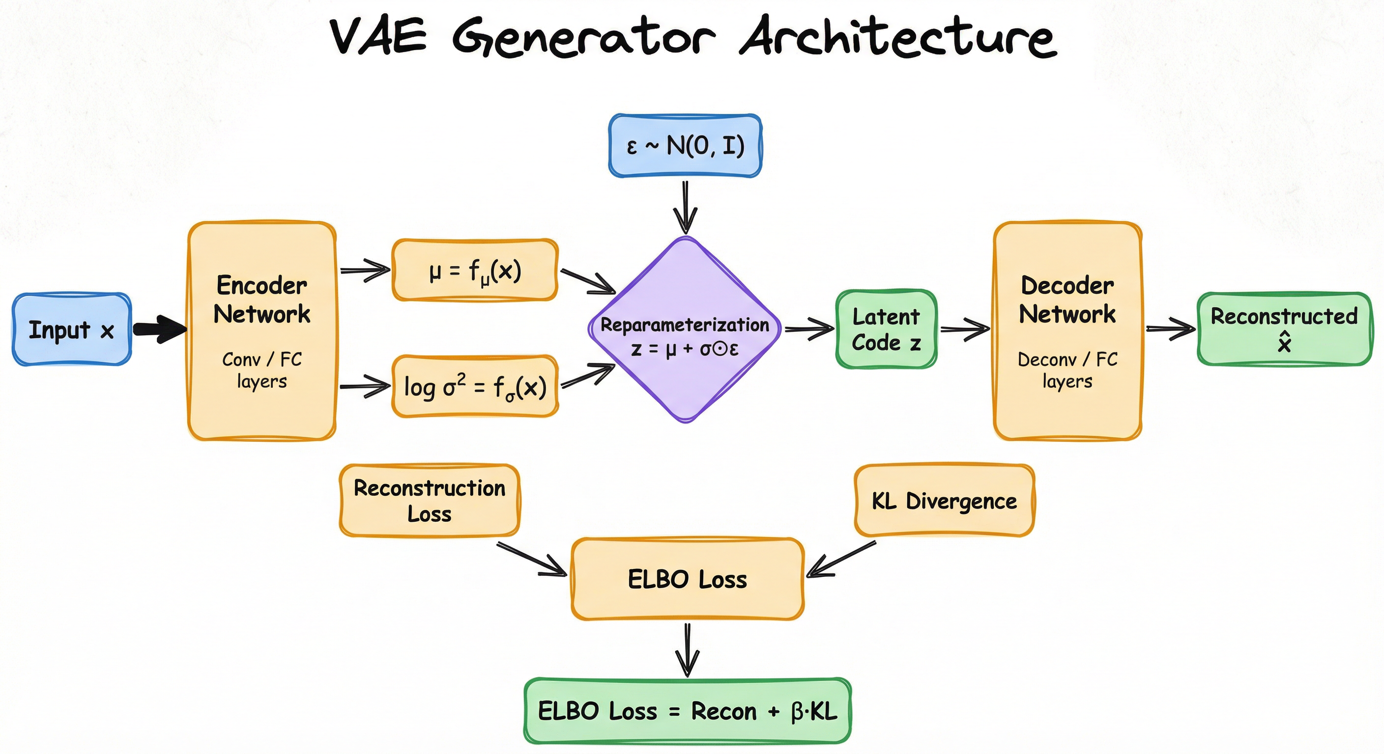
VAE Generator in ML Systems Architecture — A left-to-right flowchart showing the VAE architecture. Input data x enters the encoder network (...

At inference time for generation, only the decoder is needed: sample $z \sim \mathcal{N}(0, I)$ from the prior and pass through the decoder to produce a new sample. For reconstruction or encoding, both encoder and decoder are used.

Key Components

Encoder Network (Inference Network)

A neural network $q_\phi(z|x)$ that maps input data $x$ to the parameters of the approximate posterior distribution in latent space. For images, uses convolutional layers with stride-2 downsampling, batch normalization, and ReLU/LeakyReLU activations. The final convolutional feature map is flattened and passed through two parallel linear layers: one outputting the mean $\mu \in \mathbb{R}^d$ and one outputting the log-variance $\log \sigma^2 \in \mathbb{R}^d$ (log-variance is used instead of variance for numerical stability). The encoder is also called the recognition network or inference network because it performs approximate Bayesian inference.

Reparameterization Layer

The differentiable sampling mechanism that enables gradient flow through the stochastic latent variable. Instead of sampling $z \sim \mathcal{N}(\mu, \sigma^2)$ directly (which would block gradients), it computes $z = \mu + \sigma \odot \epsilon$ where $\epsilon \sim \mathcal{N}(0, I)$ is sampled independently. This separates the learnable parameters ( $\mu$ , $\sigma$ ) from the stochasticity ( $\epsilon$ ), enabling standard backpropagation. During inference, you can either sample (for generation diversity) or use $z = \mu$ (for deterministic encoding).

Latent Space

The low-dimensional space $\mathcal{Z} \subseteq \mathbb{R}^d$ (typically $d \in [2, 512]$ ) where the VAE learns a compressed, structured representation. Regularized by the KL divergence term to approximate $\mathcal{N}(0, I)$ , the latent space supports smooth interpolation (linear paths between codes produce gradual output changes), arithmetic (vector operations on codes correspond to semantic operations on outputs), and sampling (random draws from $\mathcal{N}(0, I)$ produce valid outputs). The structure of the latent space is what makes VAEs powerful for generation, unlike standard autoencoders.

Decoder Network (Generative Network)

A neural network $p_\theta(x|z)$ that maps latent codes $z$ to reconstructed data $\hat{x}$ . For images, uses transposed convolutions (or nearest-neighbor upsampling + convolution) with batch normalization and ReLU activations, terminating with sigmoid (for [0,1] pixel values) or tanh (for [-1,1] normalization). The decoder defines the likelihood model: Gaussian likelihood (MSE loss) for continuous data, Bernoulli likelihood (BCE loss) for binary data, or categorical likelihood (cross-entropy) for discrete data. During generation, the decoder operates alone: $\hat{x} = \text{Decoder}(z)$ where $z \sim p(z) = \mathcal{N}(0, I)$ .

Loss Function (Negative ELBO)

The training objective combines reconstruction loss and KL regularization. Reconstruction loss: $-\mathbb{E}_{q_\phi(z|x)}[\log p_\theta(x|z)]$ -- MSE for continuous outputs, BCE for binary. KL divergence: $D_{\text{KL}}(q_\phi(z|x) \| p(z))$ -- has a closed form for Gaussian-to-Gaussian. The total loss $\mathcal{L} = \text{Reconstruction} + \beta \cdot \text{KL}$ is minimized jointly over encoder ( $\phi$ ) and decoder ( $\theta$ ). The $\beta$ coefficient (standard VAE: $\beta=1$ ; $\beta$ -VAE: $\beta>1$ ) controls the reconstruction-regularization tradeoff.

Prior Distribution

The assumed distribution $p(z)$ over latent variables, typically a standard Gaussian $\mathcal{N}(0, I)$ . The prior serves as the baseline distribution from which we sample during generation. More expressive priors include Gaussian Mixture Models (VampPrior), learned autoregressive priors (VQ-VAE + PixelCNN), and normalizing flow priors (IAF-VAE) that better match the aggregate posterior and reduce the ELBO gap.

Data Flow

Training Flow:

Encode: Pass input $x$ through the encoder network to obtain latent distribution parameters: $\mu = f_\mu(x)$ , $\log \sigma^2 = f_{\log\sigma^2}(x)$ .
Sample (reparameterize): Draw $\epsilon \sim \mathcal{N}(0, I)$ and compute $z = \mu + \exp(0.5 \cdot \log \sigma^2) \odot \epsilon$ . This is the reparameterization trick -- gradients flow through $\mu$ and $\sigma$ while $\epsilon$ is treated as a constant input.
Decode: Pass the latent sample $z$ through the decoder to produce reconstruction $\hat{x} = \text{Decoder}(z)$ .
Compute loss: Calculate reconstruction loss $\| x - \hat{x} \|^2$ (or BCE) and KL divergence $\frac{1}{2}\sum(\mu^2 + \sigma^2 - \log\sigma^2 - 1)$ . Total loss = Reconstruction + $\beta \cdot$ KL.
Backpropagate: Compute gradients of total loss with respect to encoder ( $\phi$ ) and decoder ( $\theta$ ) parameters. Update both networks simultaneously with a single optimizer step.
Repeat: Continue for all minibatches across multiple epochs until convergence.

Generation Flow (Inference): Only the decoder is needed.

Sample $z \sim \mathcal{N}(0, I)$ from the prior.
Pass $z$ through the decoder: $\hat{x} = \text{Decoder}(z)$ .
Output $\hat{x}$ as the generated sample.

Interpolation Flow: Given two data points $x_1$ and $x_2$ :

Encode both: $z_1 = \mu_\phi(x_1)$ , $z_2 = \mu_\phi(x_2)$ (use means for deterministic interpolation).
Compute interpolated latents: $z_\alpha = (1-\alpha) z_1 + \alpha z_2$ for $\alpha \in [0, 1]$ .
Decode each: $\hat{x}_\alpha = \text{Decoder}(z_\alpha)$ .
The resulting sequence shows smooth transitions between $x_1$ and $x_2$ .

A left-to-right flowchart showing the VAE architecture. Input data x enters the encoder network (blue), which produces two outputs: mean mu and log-variance. These feed into the reparameterization layer (purple) along with random noise epsilon sampled from a standard Gaussian. The reparameterization layer produces the latent code z (amber), which enters the decoder network (green) to produce the reconstruction x-hat. Two loss branches are shown: reconstruction loss (comparing x and x-hat) and KL divergence loss (from mu and log-variance), which combine into the total ELBO loss (red). The diagram illustrates the differentiable sampling process that enables end-to-end backpropagation.

How to Implement

Implementation Approaches

There are three main paths to implementing VAEs in production:

Approach 1: PyTorch/TensorFlow from Scratch -- For custom architectures, implement the encoder and decoder as nn.Module subclasses, write the reparameterization trick, and define the ELBO loss manually. This provides maximum control and is straightforward because VAE training is a single-objective optimization (unlike GANs). Recommended for research or domain-specific architectures.

Approach 2: High-Level Libraries -- For tabular data, use SDV (Synthetic Data Vault) with TVAE. For images, use Pythae (a library of VAE variants including β-VAE, IWAE, VAMP, RHVAE) or PyTorch Lightning with built-in VAE templates. These abstract away boilerplate while remaining customizable.

Approach 3: Domain-Specific Frameworks -- For molecular generation, use RDKit + MolVAE. For text, use VAE-based language models. For music, use Magenta. These frameworks encode domain knowledge (chemical validity constraints, grammar rules) into the VAE architecture.

Training Stability (VAE's Key Advantage)

Unlike GANs, VAE training is remarkably stable:

Single loss function: No adversarial balancing -- just minimize negative ELBO.
Monotonic convergence: Loss decreases predictably over training. No oscillations.
Hyperparameter robustness: Learning rates of 1e-3 to 1e-4 with Adam work in most cases.
Reproducible: Same hyperparameters produce consistent results across runs.

The main training challenge is posterior collapse (see Failure Modes), addressed by KL annealing, free bits, or cyclical annealing schedules.

Cost Note: Training a convolutional VAE on 64×64 images with 50K samples takes ~30 minutes on a single RTX 4090 (~INR 40 / $0.50 in electricity). For high-resolution hierarchical VAEs like NVAE at 256×256, budget ~$ 100-300 (~INR 8,400-25,200) for training on 4x V100s over 1-2 days. This is significantly cheaper than comparable GAN training.

Convolutional VAE in PyTorch - Complete Implementation125 lines

import torch
import torch.nn as nn
import torch.nn.functional as F
import torch.optim as optim
from torch.utils.data import DataLoader
from torchvision import datasets, transforms

# Hyperparameters
latent_dim = 128
image_size = 64
channels = 3
batch_size = 128
lr = 1e-3
beta = 1.0  # KL weight (1.0 = standard VAE, >1 = β-VAE)

class Encoder(nn.Module):
    def __init__(self):
        super().__init__()
        # Conv layers: 3x64x64 -> 32x32x32 -> 64x16x16 -> 128x8x8 -> 256x4x4
        self.conv1 = nn.Conv2d(channels, 32, 4, 2, 1)
        self.conv2 = nn.Conv2d(32, 64, 4, 2, 1)
        self.conv3 = nn.Conv2d(64, 128, 4, 2, 1)
        self.conv4 = nn.Conv2d(128, 256, 4, 2, 1)
        self.bn1 = nn.BatchNorm2d(32)
        self.bn2 = nn.BatchNorm2d(64)
        self.bn3 = nn.BatchNorm2d(128)
        self.bn4 = nn.BatchNorm2d(256)
        
        # Flatten 256*4*4 = 4096 -> latent params
        self.fc_mu = nn.Linear(256 * 4 * 4, latent_dim)
        self.fc_logvar = nn.Linear(256 * 4 * 4, latent_dim)
    
    def forward(self, x):
        x = F.relu(self.bn1(self.conv1(x)))
        x = F.relu(self.bn2(self.conv2(x)))
        x = F.relu(self.bn3(self.conv3(x)))
        x = F.relu(self.bn4(self.conv4(x)))
        x = x.view(x.size(0), -1)  # Flatten
        mu = self.fc_mu(x)
        logvar = self.fc_logvar(x)
        return mu, logvar

class Decoder(nn.Module):
    def __init__(self):
        super().__init__()
        self.fc = nn.Linear(latent_dim, 256 * 4 * 4)
        self.deconv1 = nn.ConvTranspose2d(256, 128, 4, 2, 1)
        self.deconv2 = nn.ConvTranspose2d(128, 64, 4, 2, 1)
        self.deconv3 = nn.ConvTranspose2d(64, 32, 4, 2, 1)
        self.deconv4 = nn.ConvTranspose2d(32, channels, 4, 2, 1)
        self.bn1 = nn.BatchNorm2d(128)
        self.bn2 = nn.BatchNorm2d(64)
        self.bn3 = nn.BatchNorm2d(32)
    
    def forward(self, z):
        x = F.relu(self.fc(z))
        x = x.view(-1, 256, 4, 4)
        x = F.relu(self.bn1(self.deconv1(x)))
        x = F.relu(self.bn2(self.deconv2(x)))
        x = F.relu(self.bn3(self.deconv3(x)))
        x = torch.sigmoid(self.deconv4(x))  # Output [0, 1]
        return x

class VAE(nn.Module):
    def __init__(self):
        super().__init__()
        self.encoder = Encoder()
        self.decoder = Decoder()
    
    def reparameterize(self, mu, logvar):
        """Reparameterization trick: z = mu + sigma * epsilon"""
        std = torch.exp(0.5 * logvar)  # sigma = exp(0.5 * log(sigma^2))
        eps = torch.randn_like(std)     # epsilon ~ N(0, I)
        return mu + std * eps
    
    def forward(self, x):
        mu, logvar = self.encoder(x)
        z = self.reparameterize(mu, logvar)
        x_recon = self.decoder(z)
        return x_recon, mu, logvar
    
    def generate(self, num_samples, device):
        """Generate new samples from the prior."""
        z = torch.randn(num_samples, latent_dim).to(device)
        return self.decoder(z)

def vae_loss(x_recon, x, mu, logvar, beta=1.0):
    """ELBO loss = Reconstruction + beta * KL divergence."""
    # Reconstruction: Binary Cross-Entropy (pixel-wise)
    recon_loss = F.binary_cross_entropy(x_recon, x, reduction='sum')
    
    # KL divergence: closed-form for Gaussian
    # KL = -0.5 * sum(1 + log(sigma^2) - mu^2 - sigma^2)
    kl_loss = -0.5 * torch.sum(1 + logvar - mu.pow(2) - logvar.exp())
    
    return recon_loss + beta * kl_loss

# Initialize
device = torch.device('cuda' if torch.cuda.is_available() else 'cpu')
model = VAE().to(device)
optimizer = optim.Adam(model.parameters(), lr=lr)

# Training loop
for epoch in range(num_epochs):
    model.train()
    total_loss = 0
    for batch_idx, (data, _) in enumerate(dataloader):
        data = data.to(device)
        optimizer.zero_grad()
        
        x_recon, mu, logvar = model(data)
        loss = vae_loss(x_recon, data, mu, logvar, beta=beta)
        
        loss.backward()
        optimizer.step()
        total_loss += loss.item()
    
    avg_loss = total_loss / len(dataloader.dataset)
    print(f'Epoch {epoch}: Avg Loss = {avg_loss:.4f}')

# Generate new samples
model.eval()
with torch.no_grad():
    samples = model.generate(64, device)
    # samples shape: (64, 3, 64, 64)

This is a complete convolutional VAE implementation. Key design decisions:

Encoder outputs two heads: fc_mu and fc_logvar produce the mean and log-variance of the approximate posterior. Log-variance (not variance or std) is used for numerical stability -- it can be any real number, while variance must be positive.
Reparameterization trick: z = mu + exp(0.5 * logvar) * eps separates the learnable parameters from the random noise, enabling backpropagation through the sampling operation.
BCE reconstruction loss: Appropriate when pixel values are in [0, 1] (sigmoid output). For [-1, 1] outputs (tanh), use MSE loss instead.
KL closed form: The analytic KL divergence for diagonal Gaussians avoids Monte Carlo estimation noise.
Beta parameter: Set to 1.0 for standard VAE. Increase to 4-10 for disentangled β-VAE (at the cost of reconstruction quality).
Single optimizer: Unlike GANs, both encoder and decoder are updated simultaneously with the same optimizer. No alternating updates needed.

β-VAE with KL Annealing (Preventing Posterior Collapse)113 lines

import torch
import torch.nn as nn
import torch.nn.functional as F
import math

class BetaVAE(nn.Module):
    """β-VAE with cyclical KL annealing to prevent posterior collapse."""
    
    def __init__(self, input_dim, hidden_dim=512, latent_dim=64, beta=4.0):
        super().__init__()
        self.beta = beta
        self.latent_dim = latent_dim
        
        # Encoder
        self.encoder = nn.Sequential(
            nn.Linear(input_dim, hidden_dim),
            nn.BatchNorm1d(hidden_dim),
            nn.ReLU(),
            nn.Linear(hidden_dim, hidden_dim),
            nn.BatchNorm1d(hidden_dim),
            nn.ReLU(),
        )
        self.fc_mu = nn.Linear(hidden_dim, latent_dim)
        self.fc_logvar = nn.Linear(hidden_dim, latent_dim)
        
        # Decoder
        self.decoder = nn.Sequential(
            nn.Linear(latent_dim, hidden_dim),
            nn.BatchNorm1d(hidden_dim),
            nn.ReLU(),
            nn.Linear(hidden_dim, hidden_dim),
            nn.BatchNorm1d(hidden_dim),
            nn.ReLU(),
            nn.Linear(hidden_dim, input_dim),
        )
    
    def encode(self, x):
        h = self.encoder(x)
        return self.fc_mu(h), self.fc_logvar(h)
    
    def reparameterize(self, mu, logvar):
        std = torch.exp(0.5 * logvar)
        eps = torch.randn_like(std)
        return mu + std * eps
    
    def decode(self, z):
        return self.decoder(z)
    
    def forward(self, x):
        mu, logvar = self.encode(x)
        z = self.reparameterize(mu, logvar)
        x_recon = self.decode(z)
        return x_recon, mu, logvar, z

def cyclical_annealing(step, total_steps, n_cycles=4, ratio=0.5):
    """Cyclical KL annealing schedule (Fu et al., 2019).
    
    Ramps beta from 0 to 1 over `ratio` fraction of each cycle,
    then holds at 1 for the remainder. This prevents posterior
    collapse by letting the decoder learn useful representations
    before KL regularization kicks in.
    """
    cycle_length = total_steps // n_cycles
    position_in_cycle = step % cycle_length
    ramp_length = int(cycle_length * ratio)
    
    if position_in_cycle < ramp_length:
        return position_in_cycle / ramp_length
    else:
        return 1.0

def free_bits_kl(mu, logvar, free_bits=0.25):
    """Free bits: clamp KL per dimension to a minimum value.
    
    Prevents posterior collapse by ensuring each latent dimension
    encodes at least `free_bits` nats of information.
    From Kingma et al., 'Improved Variational Inference with
    Inverse Autoregressive Flow', NeurIPS 2016.
    """
    kl_per_dim = -0.5 * (1 + logvar - mu.pow(2) - logvar.exp())
    # Clamp each dimension to at least free_bits
    kl_clamped = torch.clamp(kl_per_dim, min=free_bits)
    return kl_clamped.sum(dim=-1).mean()

# Training with cyclical annealing
model = BetaVAE(input_dim=784, latent_dim=64, beta=4.0)
optimizer = torch.optim.Adam(model.parameters(), lr=1e-3)

total_steps = num_epochs * len(dataloader)
step = 0

for epoch in range(num_epochs):
    for batch_idx, (data, _) in enumerate(dataloader):
        data = data.view(-1, 784).to(device)
        
        x_recon, mu, logvar, z = model(data)
        
        # Reconstruction loss
        recon_loss = F.mse_loss(x_recon, data, reduction='sum') / data.size(0)
        
        # KL with free bits (optional)
        kl_loss = free_bits_kl(mu, logvar, free_bits=0.25)
        
        # Cyclical annealing weight
        anneal_weight = cyclical_annealing(step, total_steps)
        
        # Total loss: recon + beta * anneal_weight * KL
        loss = recon_loss + model.beta * anneal_weight * kl_loss
        
        optimizer.zero_grad()
        loss.backward()
        optimizer.step()
        step += 1

This implementation addresses the two most common VAE training challenges:

β-VAE (Higgins et al., 2017): Setting β > 1 (typically 2-10) strengthens the KL regularization, encouraging disentangled representations where individual latent dimensions capture independent factors of variation. The tradeoff: higher β means blurrier reconstructions but more interpretable, disentangled latent spaces.
Cyclical KL Annealing (Fu et al., 2019): Gradually increases the KL weight from 0 to 1 over multiple cycles. This prevents posterior collapse -- a failure mode where the KL term dominates early in training, causing the encoder to output the prior regardless of input. By initially setting KL weight to 0, the decoder first learns useful representations, then KL regularization gradually organizes the latent space.
Free Bits (Kingma et al., 2016): Ensures each latent dimension encodes at least a minimum amount of information by clamping the per-dimension KL to a floor value. This prevents the common scenario where only a few latent dimensions are active and the rest collapse to the prior.

VQ-VAE with Discrete Codebook in PyTorch99 lines

import torch
import torch.nn as nn
import torch.nn.functional as F

class VectorQuantizer(nn.Module):
    """Vector Quantization layer for VQ-VAE.
    
    Maintains a codebook of K embedding vectors. Maps continuous
    encoder outputs to the nearest codebook entry.
    """
    def __init__(self, num_embeddings=512, embedding_dim=64, commitment_cost=0.25):
        super().__init__()
        self.num_embeddings = num_embeddings
        self.embedding_dim = embedding_dim
        self.commitment_cost = commitment_cost
        
        # Codebook: K x D embedding vectors
        self.embedding = nn.Embedding(num_embeddings, embedding_dim)
        self.embedding.weight.data.uniform_(-1/num_embeddings, 1/num_embeddings)
    
    def forward(self, z_e):
        # z_e shape: (B, D, H, W) for images
        # Reshape to (B*H*W, D) for distance computation
        z_e_flat = z_e.permute(0, 2, 3, 1).contiguous().view(-1, self.embedding_dim)
        
        # Compute distances to codebook entries: ||z_e - e_k||^2
        distances = (
            torch.sum(z_e_flat ** 2, dim=1, keepdim=True)
            + torch.sum(self.embedding.weight ** 2, dim=1)
            - 2 * z_e_flat @ self.embedding.weight.t()
        )
        
        # Find nearest codebook entry
        encoding_indices = torch.argmin(distances, dim=1)
        z_q = self.embedding(encoding_indices).view(z_e.permute(0, 2, 3, 1).shape)
        z_q = z_q.permute(0, 3, 1, 2)  # Back to (B, D, H, W)
        
        # Losses
        codebook_loss = F.mse_loss(z_q.detach(), z_e)  # Move codebook to encoder
        commitment_loss = F.mse_loss(z_q, z_e.detach())  # Keep encoder near codebook
        vq_loss = codebook_loss + self.commitment_cost * commitment_loss
        
        # Straight-through estimator: copy gradients from z_q to z_e
        z_q_st = z_e + (z_q - z_e).detach()
        
        return z_q_st, vq_loss, encoding_indices

class VQVAE(nn.Module):
    def __init__(self, num_embeddings=512, embedding_dim=64):
        super().__init__()
        
        # Encoder: 3x64x64 -> 64x16x16
        self.encoder = nn.Sequential(
            nn.Conv2d(3, 32, 4, 2, 1), nn.ReLU(),
            nn.Conv2d(32, 64, 4, 2, 1), nn.ReLU(),
            nn.Conv2d(64, embedding_dim, 3, 1, 1),  # Output dim matches codebook
        )
        
        # Vector Quantizer
        self.vq = VectorQuantizer(num_embeddings, embedding_dim)
        
        # Decoder: 64x16x16 -> 3x64x64
        self.decoder = nn.Sequential(
            nn.ConvTranspose2d(embedding_dim, 64, 4, 2, 1), nn.ReLU(),
            nn.ConvTranspose2d(64, 32, 4, 2, 1), nn.ReLU(),
            nn.ConvTranspose2d(32, 3, 3, 1, 1), nn.Sigmoid(),
        )
    
    def forward(self, x):
        z_e = self.encoder(x)
        z_q, vq_loss, indices = self.vq(z_e)
        x_recon = self.decoder(z_q)
        
        recon_loss = F.mse_loss(x_recon, x)
        total_loss = recon_loss + vq_loss
        
        return x_recon, total_loss, indices
    
    def encode_to_indices(self, x):
        """Encode image to discrete codebook indices."""
        z_e = self.encoder(x)
        _, _, indices = self.vq(z_e)
        return indices

# Training
model = VQVAE(num_embeddings=512, embedding_dim=64).to(device)
optimizer = torch.optim.Adam(model.parameters(), lr=3e-4)

for epoch in range(num_epochs):
    for data, _ in dataloader:
        data = data.to(device)
        x_recon, loss, indices = model(data)
        
        optimizer.zero_grad()
        loss.backward()
        optimizer.step()

# After training, use with autoregressive prior (e.g., PixelCNN)
# for high-quality generation

VQ-VAE replaces the continuous Gaussian latent space with a discrete codebook of learned embedding vectors. Key design elements:

Vector Quantizer: Maintains a codebook of K embeddings. Each spatial location in the encoder output is mapped to the nearest codebook entry by L2 distance. This creates a discrete bottleneck.
Straight-through estimator: Gradients from the decoder cannot flow through the argmin operation, so we copy gradients directly from the quantized output to the encoder output: z_q_st = z_e + (z_q - z_e).detach().
Two auxiliary losses: Codebook loss moves embeddings toward encoder outputs. Commitment loss keeps encoder outputs near their assigned embeddings.
No KL term: VQ-VAE does not use KL divergence because the latent space is discrete. Instead, a separate autoregressive prior (PixelCNN, Transformer) is trained on the discrete indices to model $p(z)$ for generation.

VQ-VAE produces much sharper images than standard VAE because the discrete codebook prevents the averaging effect of Gaussian latent variables. Combined with PixelCNN or Transformer priors, VQ-VAE-2 achieves image quality competitive with GANs.

Configuration Example63 lines

# VAE Configuration (YAML)
model:
  architecture: conv-vae
  latent_dim: 128
  image_size: 64
  channels: 3
  variant: beta-vae  # standard | beta-vae | vq-vae

encoder:
  base_channels: 32
  num_layers: 4
  activation: relu
  normalization: batch_norm
  output_heads:
    - mu
    - logvar

decoder:
  base_channels: 32
  num_layers: 4
  activation: relu
  output_activation: sigmoid
  normalization: batch_norm

loss:
  reconstruction: bce  # bce | mse
  beta: 4.0
  kl_annealing:
    type: cyclical  # linear | cyclical | none
    warmup_epochs: 10
    n_cycles: 4
    ratio: 0.5
  free_bits: 0.25  # minimum KL per dimension (0 to disable)

training:
  batch_size: 128
  epochs: 100
  learning_rate: 1e-3
  optimizer: adam
  weight_decay: 1e-5
  scheduler:
    type: cosine
    min_lr: 1e-5

vq_vae:  # only used if variant is vq-vae
  num_embeddings: 512
  commitment_cost: 0.25
  ema_decay: 0.99  # EMA codebook update

data:
  dataset: celeba
  augmentation:
    - random_horizontal_flip
    - random_crop
    - normalize:
        mean: [0.5, 0.5, 0.5]
        std: [0.5, 0.5, 0.5]

checkpointing:
  save_every: 10
  log_reconstructions: true
  log_samples: true
  log_interpolations: true

Common Implementation Mistakes

●
Using MSE loss with sigmoid output: If the decoder outputs values in [0, 1] via sigmoid, use Binary Cross-Entropy (BCE) loss, not MSE. BCE is the correct negative log-likelihood for a Bernoulli output distribution. Using MSE with sigmoid causes gradients to vanish near 0 and 1. Conversely, if using tanh output (range [-1, 1]), MSE (Gaussian likelihood) is appropriate.
●
Not summing losses correctly: The ELBO should sum (not average) over data dimensions for the reconstruction term and sum over latent dimensions for KL. Then divide by batch size for the final loss. Averaging over data dimensions underweights reconstruction relative to KL, causing blurry outputs. Common error: using reduction='mean' in F.binary_cross_entropy when you should use reduction='sum' divided by batch size.
●
Ignoring posterior collapse: When the decoder is too powerful (e.g., autoregressive like PixelCNN), it can reconstruct perfectly without using the latent code, causing the encoder to collapse to the prior ( $q(z|x) \approx p(z)$ for all $x$ ). The latent space becomes useless. Solutions: KL annealing, free bits, or weakening the decoder (e.g., reducing receptive field).
●
Setting latent dimension too high or too low: Too few latent dimensions (e.g., 2 for complex images) create an information bottleneck that limits reconstruction quality. Too many dimensions (e.g., 1024 for MNIST) lead to unused dimensions that collapse to the prior. Start with latent_dim = 32-128 for images and 16-64 for tabular data, then tune based on the active units metric.
●
Forgetting to use log-variance instead of variance: The encoder should output $\log \sigma^2$ , not $\sigma^2$ or $\sigma$ . Log-variance can be any real number (unconstrained), while variance must be positive and standard deviation must be non-negative. Using variance directly requires an activation function (e.g., softplus) that can cause numerical issues. The reparameterization computes $\sigma = \exp(0.5 \cdot \log \sigma^2)$ .
●
Training with β too high from the start: Starting with a large β (e.g., β=10) immediately forces the latent space to match the prior before the decoder has learned useful representations. This triggers posterior collapse. Always use KL annealing: start with β=0 (or small) and increase to the target β over training. Cyclical annealing (Fu et al., 2019) repeats this ramp-up multiple times for best results.

When Should You Use This?

Use When

You need stable, reproducible training without the hyperparameter sensitivity and mode collapse issues of GANs -- VAEs converge reliably with standard Adam optimizer settings
You require density estimation or anomaly detection -- VAEs provide $\log p(x)$ (via ELBO) that directly measures how likely a sample is, enabling outlier scoring
You want a structured, interpretable latent space for downstream tasks like representation learning, interpolation, style transfer, or conditional generation
You're working with small to medium datasets (<50K samples) where GANs would overfit or mode-collapse -- VAEs generalize better from limited data
You need disentangled representations where individual latent dimensions correspond to interpretable factors of variation (using β-VAE or FactorVAE)
Your application requires both encoding and generation -- VAEs provide bidirectional mapping (encode real data to latent space AND decode latent codes to data)
You're building molecular design or drug discovery pipelines where continuous latent space navigation enables optimization of molecular properties

Avoid When

Photorealistic image quality is paramount -- standard VAEs produce blurry images due to Gaussian reconstruction loss. Use GANs, VQ-VAE + autoregressive prior, or diffusion models instead
You're generating high-resolution images (512×512+) where per-pixel losses fail to capture perceptual quality -- diffusion models or StyleGAN are better suited
Your data is purely discrete (text tokens, categorical sequences) without natural continuous representations -- autoregressive models (GPT-family) are more effective
You need maximum generation diversity without any blurriness -- GANs' adversarial loss produces sharper, more diverse samples at the cost of training stability
Speed of generation is critical and you also need high quality -- while VAEs generate fast (single forward pass), their quality lags GANs and diffusion models for complex data
You only need unconditional generation of simple data -- simpler methods like GMMs, copulas, or statistical resampling may suffice without deep learning overhead
Your team lacks expertise in probabilistic inference and latent variable models -- while VAEs train stably, debugging issues like posterior collapse requires understanding variational inference

Key Tradeoffs

Core Tradeoff: Reconstruction Quality vs. Latent Space Regularity

The ELBO's two terms pull in opposite directions. Strong reconstruction (low reconstruction loss) requires the encoder to output tight, informative distributions, while strong regularization (low KL) requires distributions to spread out and match the prior. This fundamental tension is why standard VAEs produce blurry outputs -- the Gaussian blur is a consequence of averaging over the posterior.

Aspect	VAE	GAN	Diffusion Model
Sample Quality	Good (blurry for images)	Excellent (photorealistic)	Excellent (matches GANs)
Training Stability	Excellent (single loss)	Poor (mode collapse, divergence)	Good
Training Time	Fast (30min-12h)	Moderate (2h-5 days)	Slow (1-7 days)
Inference Speed	Fast (single forward pass)	Fast (single forward pass)	Slow (20-1000 steps)
Density Estimation	Yes (ELBO lower bound)	No (implicit model)	Yes (via diffusion SDE)
Latent Space	Structured, smooth, interpretable	Unstructured	N/A (no explicit latent space)
Disentanglement	Excellent (β-VAE)	Poor	Moderate
Small Data (<10K)	Good	Poor (overfits)	Moderate

β-VAE: Reconstruction vs. Disentanglement

Increasing β forces stronger disentanglement (each latent dimension captures one factor) but degrades reconstruction quality:

β Value	Reconstruction	Disentanglement	Use Case
0.5	Better than standard	Minimal	Sharp reconstructions needed
1.0	Standard VAE	Moderate	General purpose
4.0	Blurrier	Good	Interpretable representations
10.0	Very blurry	Excellent	Factor discovery, causal analysis

Compute Cost Comparison

Task	VAE Cost	GAN Cost	Diffusion Cost
MNIST 28×28	$0.25 (₹21) / 15min	$1 (₹85) / 1h	$5 (₹420) / 3h
CelebA 64×64	$2 (₹170) / 2h	$12 (₹1,000) / 12h	$50 (₹4,200) / 1d
High-res 256×256	$50 (₹4,200) / 12h	$240 (₹20,100) / 2d	$300 (₹25,200) / 3d
Tabular 100K rows	$0.50 (₹42) / 20min	$2 (₹170) / 1h	N/A

Practitioner's Note: For most production use cases involving latent space analysis, anomaly detection, or moderate-quality generation, VAEs offer the best effort-to-value ratio. For applications demanding photorealistic quality, consider VQ-VAE-2 (which matches GAN quality with VAE stability) or diffusion models.

Alternatives & Comparisons

GAN Generator

GANs produce sharper, more photorealistic samples than standard VAEs by using an adversarial loss instead of pixel-wise reconstruction. However, GANs suffer from training instability, mode collapse, and provide no density estimation. Choose GANs when image quality is critical and you can tolerate complex training. Choose VAEs when you need stable training, latent space structure, anomaly detection, or disentangled representations.

Diffusion Generator

Diffusion models achieve GAN-level quality with better training stability by learning a gradual denoising process. They outperform standard VAEs in image quality but are 100-1000x slower at inference. Choose diffusion models for high-quality image generation where inference latency is acceptable. Choose VAEs for fast inference, explicit density estimation, or when you need an interpretable latent space.

TVAE

TVAE (Tabular VAE) is a VAE variant specialized for tabular data with mixed column types. It uses mode-specific normalization from CTGAN applied to the VAE framework. TVAE trains faster and more stably than CTGAN but may produce slightly less accurate multivariate statistics. Choose TVAE over generic VAEs for structured/tabular data with categorical and continuous columns.

CTGAN

CTGAN uses a GAN framework for tabular synthetic data, while TVAE uses a VAE framework. CTGAN can produce higher-fidelity multivariate correlations for complex tabular datasets, but is harder to train. For tabular data, CTGAN vs. TVAE is a direct comparison: CTGAN for maximum quality, TVAE for training stability and speed.

Copula Generator

Copula-based generators model multivariate dependencies using statistical copula functions (Gaussian, Clayton, Frank). They require no neural network training and are fast to fit. However, copulas assume parametric dependency structures and struggle with complex, nonlinear relationships. Choose copulas for simple tabular data with well-understood correlations. Choose VAEs for complex, nonlinear distributions.

Pros, Cons & Tradeoffs

Advantages

Stable, reproducible training: VAEs optimize a single well-defined loss (negative ELBO) that decreases monotonically. No mode collapse, no adversarial balancing, no hyperparameter knife-edge. Training converges reliably with standard Adam settings across runs.
Explicit density estimation: VAEs provide $\log p(x)$ (via ELBO lower bound), enabling anomaly detection, outlier scoring, and likelihood-based evaluation. You can answer "how likely is this sample?" -- something GANs fundamentally cannot do.
Structured, smooth latent space: The KL regularization ensures the latent space is continuous and organized. Nearby latent codes produce similar outputs, enabling smooth interpolation, latent arithmetic, and meaningful traversals. This makes VAEs ideal for representation learning and downstream tasks.
Disentangled representations (β-VAE): By increasing β, individual latent dimensions can be encouraged to capture independent, interpretable factors of variation (rotation, color, size). This enables factor discovery, controlled generation, and causal analysis -- capabilities unique to the VAE family.
Bidirectional mapping: VAEs provide both encoding ( $x \to z$ ) and decoding ( $z \to x$ ). You can encode real data into latent representations for clustering, classification, or visualization, AND generate new data from the latent space. GANs only provide the decoding direction.
Works with small datasets: VAEs generalize better than GANs from limited data (<10K samples) because the KL regularization acts as a strong prior. For Indian startups and research labs with limited labeled data, VAEs are more practical than data-hungry GANs.
Rich variant ecosystem: The VAE framework has spawned dozens of well-studied variants: β-VAE (disentanglement), CVAE (conditional generation), VQ-VAE (discrete latents, sharp images), hierarchical VAE (multi-scale), NVAE (GAN-competitive quality). Each addresses specific limitations while maintaining the core stability.

Disadvantages

Blurry sample quality: Standard VAEs with Gaussian decoders produce blurry images because MSE/BCE loss averages over reconstruction uncertainty. The Gaussian likelihood penalizes pixel-level deviations rather than perceptual quality. VQ-VAE and perceptual loss VAEs address this but add complexity.
Posterior collapse: When the decoder is powerful enough to model $p(x)$ without the latent code, the encoder collapses to the prior ( $q(z|x) \approx p(z)$ ), making the latent space useless. This is especially common with autoregressive decoders or very deep architectures. Requires KL annealing, free bits, or architectural constraints.
ELBO is a lower bound, not exact: The training objective is a lower bound on $\log p(x)$ , not the true likelihood. The gap depends on how well $q(z|x)$ approximates $p(z|x)$ . This means a lower ELBO doesn't always mean a better generative model. Tighter bounds (IWAE) or more flexible posteriors (normalizing flows) partially address this.
Limited expressiveness with standard Gaussian posterior: Assuming $q(z|x) = \mathcal{N}(\mu, \sigma^2 I)$ restricts the posterior to unimodal, axis-aligned Gaussians. Complex true posteriors with multiple modes or correlations are poorly approximated. Normalizing flow posteriors (IAF-VAE) or mixture posteriors improve this.
Reconstruction-regularization tradeoff: The ELBO's two terms inherently conflict. You cannot simultaneously achieve perfect reconstruction AND perfect KL match to the prior. This fundamental tension limits overall quality. There is no free lunch -- sharper images require sacrificing latent space regularity, and vice versa.
Evaluation challenges: While ELBO provides a training signal, it's not a reliable metric for comparing different VAE architectures or for measuring generation quality. FID scores for VAEs are typically 2-5x worse than comparable GANs. Separate evaluation (FID, visual inspection, downstream task performance) is needed.
Latent space underutilization: In high-dimensional latent spaces, many dimensions collapse to the prior and encode no information. The model effectively uses a lower-dimensional subspace. Tracking active units (AU) and using techniques like free bits are needed to maximize latent space utilization.

Increase KL weight (higher β) to force better prior matching at the cost of reconstruction quality. Use more expressive priors: Replace $\mathcal{N}(0, I)$ with a VampPrior (mixture of approximate posteriors), a learned GMM prior, or a normalizing flow prior that better matches the aggregate posterior shape. Two-stage training: First train the VAE, then fit a more flexible prior (e.g., a normalizing flow) to the aggregate posterior. Rejection sampling: At generation time, reject samples that fall in low-density regions of the aggregate posterior.

Placement in an ML System

Where VAEs Fit in Production ML Systems

VAEs serve multiple roles in production ML pipelines, often simultaneously:

1. Synthetic Data Generation: Train a VAE on real data, then sample from the prior to generate unlimited synthetic samples. Unlike GANs, VAE training is stable and reproducible, making it suitable for automated pipelines. Use cases: data augmentation for rare classes, privacy-preserving data sharing (with differential privacy), generating test data for QA environments.

2. Anomaly Detection: The ELBO provides a natural anomaly score -- data points with low ELBO (high reconstruction error or high KL divergence) are likely outliers. This is used in fraud detection (Razorpay-style fintech systems), manufacturing defect detection, and medical image screening (Qure.ai-style applications).

3. Representation Learning: The encoder maps data to a structured latent space useful for downstream tasks. Latent representations can be used for clustering, similarity search, or as features for classifiers. β-VAE latent codes are particularly useful because disentangled dimensions are independently interpretable.

4. Conditional Generation (CVAE): By conditioning on labels or attributes, CVAEs generate data matching specific criteria. In ML systems, this enables targeted data augmentation ("generate more samples of rare class X"), controlled synthetic data ("generate patient records with diabetes and age > 60"), and what-if analysis.

Example Pipeline: A fintech company in India trains a VAE on anonymized transaction data. The system serves three purposes: (1) anomaly detection -- flag transactions with low ELBO as potential fraud; (2) synthetic data -- generate fake transaction records for developer testing environments under RBI data localization rules; (3) representation learning -- use latent codes as features for a downstream credit scoring model.

Pipeline Stage

Data Generation / Representation Learning

Upstream

Real training data collection and preprocessing
Data cleaning and normalization
Feature engineering (for tabular VAEs)
Image preprocessing (resize, normalize to [0,1] or [-1,1])

Downstream

Synthetic data quality evaluation (FID, statistical tests)
Anomaly detection systems (using ELBO as anomaly score)
Downstream model training (using synthetic or augmented data)
Representation learning and clustering (using latent space)
Privacy-preserving data sharing (synthetic records)

Scaling Bottlenecks

Training Bottlenecks

VAE training is compute-bound during the encoder-decoder forward/backward pass. Unlike GANs, there is no alternating optimization -- the entire model is updated in a single step, making distributed training straightforward with standard data parallelism.

Memory: The main bottleneck is storing intermediate activations for both encoder and decoder during backpropagation. For high-resolution images (256×256+), gradient checkpointing reduces memory at the cost of ~30% slower training. A hierarchical VAE (NVAE) with 30+ latent layers requires 24-40 GB GPU memory.

Latent dimensionality: Higher latent dimensions increase the KL computation and the decoder's input size, but this is typically a small fraction of total compute. The bottleneck is almost always the convolutional/attention layers.

Inference Bottlenecks

VAE inference is fast -- a single forward pass through the decoder. For batch generation, throughput scales linearly with batch size up to GPU memory limits. A convolutional VAE generates ~5,000 64×64 images per second on a single V100.

Latent space navigation for large-scale generation requires sampling strategies. Uniform sampling from $\mathcal{N}(0, I)$ works but may undersample rare modes. For production, use importance-weighted sampling or fit a more complex prior to the aggregate posterior.

Large-Scale Deployment

For serving, only the decoder is needed (encoder is discarded unless encoding/anomaly detection is required). The decoder is typically 5-15M parameters -- easily served on CPU for moderate throughput or GPU for high throughput. Quantizing to FP16 halves memory with negligible quality loss.

Production Case Studies

DeepMind (Alphabet)AI Research / Drug Discovery

DeepMind's work on protein structure prediction (AlphaFold) and related generative modeling research has leveraged VAE-based approaches for learning compact representations of protein structures. VAE-based models learn latent spaces over molecular conformations, enabling exploration of protein design space. The latent space structure allows interpolation between known protein folds to hypothesize novel structures.

Outcome:

VAE-based generative models for molecular design have enabled 10-100x faster exploration of chemical space compared to brute-force screening. In drug discovery pipelines, this translates to reducing candidate molecule screening from months to days. Indian pharmaceutical companies (Dr. Reddy's, Biocon) are exploring similar VAE-based approaches for generic drug molecule optimization.

SpotifyMusic / Entertainment

Spotify Research's official publication on FS-VAE (Fast-Slow Variational Autoencoder) presented at WSDM 2022, which uses sequential and non-sequential encoders to model user listening patterns by capturing both long-term preferences and short-term taste changes.

Outcome:

FS-VAE significantly improved prediction accuracy for next track selection compared to baseline models; combines variational autoencoder architecture with fast-moving (session-based) and slow-moving (historical) feature encoders for personalized music recommendations.

NVIDIA ResearchTechnology / AI Research

NVIDIA's NVAE (Nouveau VAE) demonstrated that hierarchical VAEs can achieve image quality competitive with GANs. NVAE uses a deep hierarchical latent structure with residual cells, spectral regularization, and depth-wise separable convolutions. The model achieves state-of-the-art density estimation on CIFAR-10 and CelebA while generating high-quality 256×256 images.

Outcome:

NVAE achieved FID of 51.7 on CelebA 256×256 (compared to 62.2 for previous best VAE), narrowing the gap with GANs significantly. The model demonstrated that careful architectural design -- not just the loss function -- determines VAE image quality. NVAE's techniques (spectral regularization, residual latent cells) have been adopted by subsequent hierarchical VAE research.

RazorpayFintech (India)

Razorpay's ML team explores VAE-based approaches for two key applications: (1) fraud detection using the ELBO as an anomaly score to flag suspicious payment transactions, and (2) synthetic data generation for creating realistic test transaction datasets that comply with RBI data localization requirements. The VAE latent space clusters transactions by risk profile, enabling targeted monitoring.

Outcome:

VAE-based anomaly detection processes 100M+ transactions monthly with sub-10ms latency per transaction (decoder-only inference). The synthetic data pipeline generates privacy-preserving test datasets that enable Razorpay's engineering teams to develop and test payment features without accessing real customer transaction data, supporting RBI compliance and PCI-DSS requirements.

Tooling & Ecosystem

Pythae

PythonOpen Source

A comprehensive Python library implementing 20+ VAE variants including standard VAE, β-VAE, IWAE, VQ-VAE, VAMP, RHVAE, SVAE, and more. Provides unified training pipelines, evaluation metrics, and model comparison tools. The best resource for benchmarking and experimenting with different VAE architectures.

Synthetic Data Vault (SDV)

PythonOpen Source

Production-grade library for generating synthetic tabular data. Includes TVAE (Tabular VAE) alongside CTGAN and copula-based synthesizers. Provides metadata-driven configuration, quality metrics (Column Shapes, Column Pair Trends), and constraint handling. The standard tool for tabular synthetic data.

PyTorch Lightning + VAE Template

PythonOpen Source

PyTorch Lightning provides structured training loops that simplify VAE implementation. The community maintains VAE templates with built-in logging, distributed training, and checkpointing. Reduces boilerplate while maintaining full flexibility for custom architectures.

Disentanglement Library (disentanglement_lib)

PythonOpen Source

Google Research library for training and evaluating disentangled representations, primarily through β-VAE and its variants. Includes standardized disentanglement metrics (DCI, SAP, Factor VAE metric), benchmark datasets (dSprites, 3D Shapes), and reproducible training pipelines.

TorchMetrics

PythonOpen Source

Includes implementations of FID (Frechet Inception Distance), IS (Inception Score), and other generative model evaluation metrics. GPU-accelerated and compatible with PyTorch Lightning. Essential for quantitatively evaluating VAE generation quality against baselines.

Hugging Face Diffusers (VAE components)

PythonOpen Source

While primarily for diffusion models, Hugging Face Diffusers includes pretrained VAE encoder-decoders used in Stable Diffusion (the KL-autoencoder). These VAEs map images to compact latent spaces and back, providing production-ready encoder-decoder pairs that can be used standalone for representation learning or image compression.

Research & References

Auto-Encoding Variational Bayes

Kingma & Welling (2013)ICLR 2014

The foundational VAE paper that introduced the framework of amortized variational inference with neural networks. Derived the ELBO, proposed the reparameterization trick for differentiable sampling through Gaussian latent variables, and demonstrated generation on MNIST and Frey Face datasets. One of the most cited papers in deep generative modeling.

Stochastic Backpropagation and Approximate Inference in Deep Generative Models

Rezende, Mohamed & Wissner-Gross (2014)ICML 2014

Independently derived the same variational autoencoder framework as Kingma & Welling, arriving at the reparameterization trick through a different mathematical path (stochastic backpropagation). Also introduced the idea of using normalizing flows to create more flexible approximate posteriors, which later became a major research direction.

β-VAE: Learning Basic Visual Concepts with a Constrained Variational Framework

Higgins, Matthey, Pal, Burgess, Glorot, Botvinick, Mohamed & Lerchner (2017)ICLR 2017

Introduced the β-VAE by adding a hyperparameter β > 1 to the KL term, discovering that stronger regularization encourages disentangled representations where individual latent dimensions correspond to interpretable factors of variation. Proposed the disentanglement metric and demonstrated on dSprites and CelebA that β-VAE discovers rotation, scale, position, and shape factors without supervision.

Neural Discrete Representation Learning (VQ-VAE)

van den Oord, Vinyals & Kavukcuoglu (2017)NeurIPS 2017

Introduced Vector Quantized VAE (VQ-VAE) replacing the continuous Gaussian latent space with a discrete codebook of learned embeddings. Uses straight-through estimation for gradient flow through the quantization step. Combined with a PixelCNN prior over discrete codes, VQ-VAE achieves sharper image generation than continuous VAEs and enables high-quality speech synthesis.

Generating Diverse High-Fidelity Images with VQ-VAE-2

Razavi, van den Oord & Vinyals (2019)NeurIPS 2019

Extended VQ-VAE to a multi-scale hierarchical architecture (VQ-VAE-2) that generates diverse, high-fidelity 1024×1024 images. Uses a top-level codebook for global structure and a bottom-level codebook for local details, each with its own autoregressive prior. Achieved FID competitive with BigGAN while maintaining the stable training of VAEs.

NVAE: A Deep Hierarchical Variational Autoencoder

Vahdat & Kautz (2020)NeurIPS 2020

Demonstrated that carefully designed hierarchical VAEs can achieve GAN-competitive image quality. NVAE uses deep residual cells, spectral regularization, and depth-wise separable convolutions across 30+ hierarchical latent layers. Achieved state-of-the-art density estimation on CIFAR-10 (2.91 bits/dim) and competitive FID on CelebA 256×256 (51.7).

Cyclical Annealing Schedule: A Simple Approach to Mitigating KL Vanishing

Fu, Li, Gan, Chen, Henao & Carin (2019)NAACL 2019

Proposed cyclical KL annealing as a solution to posterior collapse in VAE training. Instead of linearly increasing the KL weight once, the schedule cycles between 0 and 1 multiple times during training. Each cycle allows the model to first learn useful representations (low KL weight) then organize the latent space (high KL weight). Demonstrated significant improvements in text generation and dialogue modeling.

Interview & Evaluation Perspective

Common Interview Questions

●
Explain how VAEs work. What is the ELBO and why do we optimize it?
●
What is the reparameterization trick and why is it necessary?
●
Compare VAEs to GANs. When would you choose one over the other?
●
What is posterior collapse and how do you prevent it?
●
Explain the difference between β-VAE and standard VAE. What does disentanglement mean?
●
How does VQ-VAE differ from standard VAE? Why does it produce sharper images?
●
How would you use a VAE for anomaly detection in a production system?
●
Design a privacy-preserving synthetic data system using VAEs for a fintech company.

Key Points to Mention

●
VAEs learn a latent variable model by maximizing the ELBO: $\text{ELBO} = \mathbb{E}_{q(z|x)}[\log p(x|z)] - D_{\text{KL}}(q(z|x) \| p(z))$ . The ELBO lower-bounds the intractable log-likelihood $\log p(x)$ . The gap is the KL between approximate and true posteriors.
●
The reparameterization trick ( $z = \mu + \sigma \odot \epsilon$ , $\epsilon \sim \mathcal{N}(0,I)$ ) enables backpropagation through the stochastic sampling step by separating learnable parameters from randomness.
●
VAEs provide three things GANs cannot: (1) density estimation for anomaly detection, (2) structured latent space for representation learning, (3) stable, reproducible training. GANs provide one thing VAEs struggle with: photorealistic sample quality.
●
Posterior collapse occurs when the decoder ignores the latent code. The encoder outputs the prior for all inputs, making the latent space useless. Solutions: KL annealing (linear or cyclical), free bits (minimum KL per dimension), weaker decoder.
●
β-VAE with β > 1 encourages disentangled representations where each latent dimension captures one independent factor of variation. At β = 4-10, you can discover factors like rotation, lighting, and color without supervision, at the cost of blurrier reconstructions.
●
VQ-VAE replaces the Gaussian latent space with a discrete codebook, avoiding the averaging effect that causes blur. Combined with an autoregressive prior (PixelCNN/Transformer), VQ-VAE achieves GAN-competitive image quality while maintaining stable VAE training.
●
For anomaly detection: encode input $x$ , compute ELBO (or just reconstruction error). Low ELBO = data point is unlikely under the learned distribution = potential anomaly. This provides a principled, calibrated anomaly score.

Pitfalls to Avoid

●
Claiming VAEs generate as well as GANs for images -- standard VAEs produce blurrier outputs. Acknowledge the reconstruction-regularization tradeoff. Mention VQ-VAE and hierarchical VAEs if pressed on quality.
●
Confusing the ELBO with the true likelihood. The ELBO is a lower bound; a lower ELBO value doesn't always mean a better generative model because the bound gap can vary. Show awareness of tighter bounds (IWAE) and their tradeoffs.
●
Saying the KL divergence 'measures how different two distributions are' without specifying it's asymmetric: $D_{\text{KL}}(q \| p) \neq D_{\text{KL}}(p \| q)$ . The VAE minimizes $D_{\text{KL}}(q(z|x) \| p(z))$ , which tends to be mode-covering (spreading $q$ to cover all of $p$ ).
●
Not mentioning posterior collapse as the primary failure mode. This is the single most important practical challenge in VAE training, and interviewers expect you to know solutions (KL annealing, free bits).
●
Describing VAEs as 'just autoencoders with noise' -- this misses the probabilistic foundation. VAEs are principled latent variable models trained with variational inference. The mathematical framework (ELBO, variational posterior, prior matching) is what makes them useful beyond compression.

Senior-Level Expectation

A senior/staff engineer should discuss VAEs at three levels: (1) Mathematical: Derive the ELBO from Jensen's inequality or the KL decomposition. Explain why the reparameterization trick works and when it fails (non-Gaussian posteriors -- use normalizing flows or score function estimator). Discuss the information-theoretic interpretation: rate (KL) vs. distortion (reconstruction) tradeoff. (2) Architecture: Compare VAE variants -- β-VAE for disentanglement, VQ-VAE for discrete representation and sharp generation, hierarchical VAE (NVAE, VDVAE) for multi-scale modeling. Discuss when each variant is appropriate and their computational tradeoffs. (3) System Design: For a production synthetic data system, design the full pipeline: VAE training on sensitive data (with optional differential privacy), quality evaluation (FID, statistical tests, downstream task performance), privacy auditing (membership inference attacks), and deployment (encoder for anomaly detection at inference time, decoder for batch synthetic data generation). Estimate costs in INR/USD, latency budgets, and scaling requirements. Address the reconstruction-regularization tradeoff with practical solutions (perceptual loss, VQ-VAE) and explain when a VAE is the right choice versus GANs or diffusion models.

Summary

What We Covered

Variational Autoencoders (VAEs), introduced by Kingma & Welling in 2013, are probabilistic generative models that learn latent variable representations through variational inference. The encoder maps data to the parameters of a distribution $q(z|x) = \mathcal{N}(\mu, \sigma^2)$ in latent space, and the decoder generates data from sampled latent codes. Training maximizes the Evidence Lower Bound (ELBO), which balances reconstruction quality against latent space regularization through KL divergence.

The reparameterization trick ( $z = \mu + \sigma \odot \epsilon$ , $\epsilon \sim \mathcal{N}(0,I)$ ) enables gradient-based optimization through the stochastic sampling step. The VAE framework has spawned powerful variants: β-VAE (β > 1 encourages disentangled representations where each latent dimension captures one independent factor), VQ-VAE (discrete codebook latents that produce sharper images by avoiding Gaussian averaging), CVAE (conditional generation given labels or attributes), and hierarchical VAEs (NVAE, VDVAE) that stack multiple latent layers for multi-scale representation and GAN-competitive image quality.

VAEs' key strengths are stable training (single loss, monotonic convergence, no mode collapse), density estimation (ELBO as anomaly score), structured latent space (smooth interpolation, arithmetic, disentanglement), and bidirectional mapping (encode and decode). Their main weakness is blurry sample quality for images due to the reconstruction-regularization tradeoff, though VQ-VAE and hierarchical architectures largely address this. Posterior collapse -- where the encoder ignores the input and outputs the prior -- is the primary failure mode, mitigated by KL annealing, free bits, and cyclical schedules.

For production deployments, VAEs serve as synthetic data generators (privacy-preserving tabular data for fintech/healthcare compliance), anomaly detectors (ELBO-based scoring for fraud detection and medical screening), and representation learners (structured latent spaces for clustering, search, and downstream models). Training costs are 2-10x lower than comparable GANs: a convolutional VAE on 64×64 images trains in ~2 hours for $2 / ₹170, while high-resolution hierarchical VAEs require ~$ 50-300 / ₹4,200-25,200 for 1-2 days on multi-GPU setups. VAEs are the right choice when you need stable training, density estimation, or interpretable latent spaces; defer to GANs or diffusion models when photorealistic image quality is the primary requirement.

Concept Snapshot

Why This Concept Exists

The Challenge of Tractable Generative Modeling

The Variational Inference Breakthrough

Evolution: From Blurry Samples to State-of-the-Art

Core Intuition & Mental Model

The Postal Service Analogy

Why Randomness Enables Generation

The Reconstruction-Regularization Dance

Technical Foundations

The Generative Model

The Intractability Problem

Variational Inference and ELBO

ELBO Decomposition

Closed-Form KL for Gaussians

The Reparameterization Trick

β-VAE Objective

VQ-VAE: Discrete Latent Variables

Internal Architecture

Key Components

Data Flow

How to Implement

Implementation Approaches

Training Stability (VAE's Key Advantage)

Common Implementation Mistakes

When Should You Use This?

Use When

Avoid When

Key Tradeoffs

Core Tradeoff: Reconstruction Quality vs. Latent Space Regularity

β-VAE: Reconstruction vs. Disentanglement

Compute Cost Comparison

Alternatives & Comparisons

Pros, Cons & Tradeoffs

Advantages

Disadvantages

Failure Modes & Debugging

Posterior Collapse

Blurry Reconstruction / Generation

KL Vanishing / Over-Regularization

Codebook Collapse (VQ-VAE)

Latent Space Holes

Placement in an ML System

Where VAEs Fit in Production ML Systems

Pipeline Stage

Upstream

Downstream

Scaling Bottlenecks

Production Case Studies

Tooling & Ecosystem

Research & References

Interview & Evaluation Perspective

Common Interview Questions

Key Points to Mention

Pitfalls to Avoid

Senior-Level Expectation

Summary

What We Covered

Related Blocks & Further Reading

Related ML Blocks

Further Reading