Diffusion Generator in Machine Learning
Diffusion models have rapidly become the dominant paradigm in generative AI, powering systems like Stable Diffusion, DALL-E 2/3, Imagen, and Midjourney. The core idea is deceptively simple: take real data, gradually corrupt it with noise until it becomes pure static, then train a neural network to reverse that corruption step by step. At generation time, start with random noise and iteratively denoise it into a coherent sample.
What makes diffusion models remarkable is their combination of training stability, sample quality, and controllability -- three properties that previously seemed to be in fundamental tension. GANs produce sharp images but suffer from mode collapse and training instability. VAEs train stably but produce blurry outputs. Diffusion models achieve GAN-level quality with VAE-level stability, though at the cost of slower inference due to their iterative sampling process.
The mathematical foundations trace back to non-equilibrium thermodynamics (Sohl-Dickstein et al., 2015), but the practical breakthrough came with Denoising Diffusion Probabilistic Models (DDPM) by Ho, Jain, and Abbeel in 2020. DDPM showed that a simple noise-prediction objective -- train a U-Net to predict the noise added at each step -- could generate images rivaling GANs. Since then, innovations like latent diffusion (operating in compressed latent space rather than pixel space), classifier-free guidance (steering generation with text or class conditioning), and DDIM (faster deterministic sampling) have made diffusion models practical for production.
Today, diffusion generators are not limited to images. TabDDPM applies the diffusion framework to tabular synthetic data, outperforming GAN-based methods like CTGAN. Audio diffusion models power music and speech synthesis. Molecular diffusion models generate drug candidates. From Flipkart's product image generation pipelines to ISRO's satellite imagery augmentation, diffusion models are becoming the default choice for high-fidelity synthetic data generation across modalities.
Concept Snapshot
- What It Is
- A generative model that learns to produce data by training a neural network to reverse a gradual noising process, transforming random Gaussian noise into structured samples through iterative denoising steps.
- Category
- Data Generation
- Complexity
- Advanced
- Inputs / Outputs
- Inputs: training dataset (for training) or random Gaussian noise + optional conditioning signal such as text prompt or class label (for generation). Outputs: high-fidelity synthetic samples matching the training data distribution.
- System Placement
- Sits in the data generation and augmentation stage of ML pipelines, producing synthetic training data, augmenting limited datasets, or generating content for downstream tasks like classification, segmentation, or retrieval.
- Also Known As
- Denoising Diffusion Model, DDPM, Score-Based Generative Model, Diffusion Probabilistic Model, Latent Diffusion Model
- Typical Users
- ML Engineers, Data Scientists, Computer Vision Engineers, Research Scientists, Generative AI Engineers, Privacy Engineers
- Prerequisites
- Deep neural networks (U-Net architecture), Gaussian distributions and Markov chains, Variational inference basics, PyTorch or TensorFlow fundamentals, Basic probability theory (KL divergence, ELBO)
- Key Terms
- forward processreverse processnoise schedulescore matchingclassifier-free guidancelatent diffusionDDPMDDIMdenoising U-Netvariational lower bound
Why This Concept Exists
The Generative Modeling Trilemma
Before diffusion models, generative modeling faced an uncomfortable trilemma. You could pick any two of the following, but not all three:
- High sample quality (sharp, realistic outputs)
- Stable training (no mode collapse, no hyperparameter sensitivity)
- Mode coverage (diverse outputs capturing the full data distribution)
GANs excelled at sample quality but suffered from training instability and mode collapse -- the generator would often learn to produce only a handful of realistic samples, ignoring entire modes of the data distribution. VAEs trained stably with full mode coverage but produced blurry outputs because the pixel-wise reconstruction loss averaged over possibilities rather than committing to one sharp realization. Autoregressive models (PixelCNN, GPT) achieved good quality and coverage but were painfully slow at generation due to sequential sampling.
Diffusion models broke through this trilemma.
The Thermodynamic Inspiration
The foundational idea came from non-equilibrium statistical mechanics. In 2015, Sohl-Dickstein, Weiss, Maheswaranathan, and Ganguli published "Deep Unsupervised Learning using Nonequilibrium Thermodynamics," drawing an analogy between data generation and thermodynamic processes. Just as a physical system can be driven from equilibrium (structured state) to maximum entropy (random noise) through a sequence of small perturbations, data can be gradually destroyed by adding noise. The key insight: if each noise-adding step is small enough, the reverse step is also approximately Gaussian and can be learned by a neural network.
This 2015 paper was ahead of its time -- the results were modest, and GANs dominated the conversation. It took five more years for the idea to mature.
The DDPM Breakthrough (2020)
Jonathan Ho, Ajay Jain, and Pieter Abbeel at UC Berkeley published "Denoising Diffusion Probabilistic Models" (DDPM) in 2020, demonstrating that diffusion models could match or exceed GAN quality on image generation benchmarks. The key simplification was training the neural network to predict the noise that was added at each step, rather than predicting the denoised image directly. Combined with a carefully designed noise schedule and a U-Net architecture, this produced state-of-the-art FID scores on CIFAR-10 and LSUN.
DDPM's success sparked an avalanche of follow-up work:
- Improved DDPM (Nichol & Dhariwal, 2021): Learned variance schedules and cosine noise schedules for better log-likelihood
- DDIM (Song, Meng & Ermon, 2021): Deterministic sampling with 10-50x fewer steps
- Score SDE (Song et al., 2021): Unified framework connecting diffusion models and score-based generative models through stochastic differential equations
- Latent Diffusion Models (Rombach et al., 2022): Moved diffusion to a compressed latent space, enabling high-resolution generation at tractable compute costs -- this became Stable Diffusion
- Classifier-Free Guidance (Ho & Salimans, 2022): Enabled powerful text conditioning without a separate classifier
Indian Context: IIT Bombay, IIT Hyderabad, and IISc Bangalore research groups have published work on diffusion models for Indian language document synthesis, medical imaging (chest X-ray generation for AIIMS datasets), and satellite image super-resolution. Indian startups like Haptik and Vernacular.ai have explored diffusion-based data augmentation for low-resource Indian language ASR systems.
Core Intuition & Mental Model
The Sandcastle Analogy
Imagine you build a sandcastle on the beach. Every hour, the tide comes in a little further, eroding the castle slightly. After many hours, the castle is gone -- just flat, featureless sand. Now imagine you recorded a time-lapse video of this erosion. If you play the video backwards, you see structure spontaneously emerging from flat sand: first vague mounds, then walls, then towers and turrets, until you have a complete castle.
Diffusion models work exactly like this backwards video. The forward process is the tide -- it gradually adds noise to data until it becomes featureless Gaussian noise. The reverse process is the video played backwards -- a neural network that has learned to remove noise step by step, reconstructing structure from chaos.
The crucial insight: each individual erosion step is tiny and predictable (just add a small amount of Gaussian noise). Because each step is small, the reverse step is also approximately Gaussian, and a neural network can learn to predict it. You don't need to learn the entire forward-to-reverse mapping at once -- just learn to undo one small noise step at a time.
Why Does This Work So Well?
Three reasons make diffusion models surprisingly effective:
1. Decomposition of difficulty. Generating a complex image from scratch is incredibly hard. But removing a tiny amount of noise from an already-almost-clean image? That's easy. Diffusion models decompose the hard problem of generation into many easy denoising subproblems. Each step only needs to make a small, local correction.
2. Stable training objective. Unlike GANs, where the loss landscape is a saddle point of a minimax game, diffusion models optimize a simple, well-behaved loss: mean squared error between predicted noise and actual noise. No adversarial dynamics, no mode collapse, no careful balancing of two competing networks.
3. Full distribution coverage. Because the forward process covers the entire data distribution with noise (every data point eventually becomes Gaussian noise), the reverse process must learn to reconstruct all modes. There's no mechanism for the model to "forget" parts of the distribution the way a GAN generator can mode-collapse.
The Noise Schedule: The Conductor of the Orchestra
The noise schedule controls how quickly data is corrupted in the forward process. Think of it as the conductor setting the tempo:
- Linear schedule (original DDPM): increases linearly from to . Simple but wastes compute on nearly-noiseless early steps.
- Cosine schedule (Improved DDPM): . Spends more time at intermediate noise levels where the model learns the most.
- Learned schedule: Let the model learn optimal noise levels during training.
Getting the schedule right matters enormously. Too aggressive (noise added too fast), and the model doesn't have enough intermediate steps to learn the reverse. Too conservative (noise added too slowly), and you waste compute on steps where the model has little to learn.
Mental Model: Think of the noise schedule as a curriculum. A good teacher starts with easy questions (remove a tiny bit of noise from a nearly clean image) and gradually increases difficulty (reconstruct structure from very noisy inputs). The cosine schedule is a better curriculum than the linear schedule because it spends more time on medium-difficulty denoising tasks.
Technical Foundations
The Forward Process (Adding Noise)
Given a data point , the forward process defines a Markov chain that gradually adds Gaussian noise over timesteps:
where is the variance schedule with . After steps (typically ), -- the data has been completely destroyed.
Defining and , we can sample directly from without iterating through all intermediate steps:
This is the reparameterization trick: where .
The Reverse Process (Removing Noise)
The reverse process is a learned Markov chain running backwards from to :
The neural network parameterized by predicts the mean and optionally the variance of each reverse step. In DDPM, the variance is fixed to where or .
The Noise Prediction Objective
Instead of predicting directly, DDPM reparameterizes the mean as:
where is a neural network that predicts the noise that was added. The simplified training objective becomes:
This is just mean squared error between the actual noise and the predicted noise . Despite its simplicity, this objective works remarkably well.
Connection to Score Matching
The noise prediction is directly related to the score function -- the gradient of the log-density with respect to the data:
Song et al. (2021) showed that diffusion models and score-based generative models are unified through stochastic differential equations (SDEs). The forward process is described by an SDE:
and the reverse process by:
where is the score function estimated by the neural network.
Classifier-Free Guidance
For conditional generation (e.g., text-to-image), classifier-free guidance (Ho & Salimans, 2022) trains a single model that can operate both conditionally and unconditionally. During training, the conditioning signal is randomly dropped (replaced with null ) with probability (typically 10-20%). At inference, the guided score is:
where is the guidance scale that controls the strength of conditioning. Higher produces samples more aligned with the conditioning but with less diversity. Typical values: for class conditioning, for text-to-image.
DDIM: Deterministic Sampling
DDIM (Song, Meng & Ermon, 2021) provides a non-Markovian reverse process that enables deterministic sampling with far fewer steps. The DDIM update rule:
Setting gives a fully deterministic mapping from noise to data, enabling 10-50 step generation versus DDPM's 1000 steps.
Key Insight: The beauty of the DDPM training objective is its simplicity -- predict the noise, minimize MSE. No adversarial dynamics, no posterior collapse, no complex loss balancing. This simplicity is precisely why diffusion models scale so well to larger datasets and higher resolutions.
Internal Architecture
The architecture of a diffusion generator has two main configurations: pixel-space diffusion (operating directly on images/data) and latent diffusion (operating in a compressed representation). Modern production systems almost exclusively use latent diffusion for computational efficiency.
In pixel-space DDPM, a U-Net with attention layers takes a noisy image and a timestep embedding as input and predicts the noise . The U-Net's encoder-decoder structure with skip connections is ideal for this task: the encoder captures global context while skip connections preserve fine-grained spatial details needed for denoising.
In latent diffusion (the architecture behind Stable Diffusion), a pretrained VAE encoder first compresses images into a low-dimensional latent space (typically 4x-8x spatial downsampling). The U-Net denoiser operates in this compressed space, dramatically reducing compute. A VAE decoder maps the denoised latent back to pixel space. For text conditioning, a text encoder (e.g., CLIP) converts prompts into embeddings that are injected into the U-Net via cross-attention layers.
The latent diffusion approach reduces the spatial dimensions by 8x in each direction (e.g., 512x512 images become 64x64 latent maps with 4 channels), cutting the number of elements the U-Net processes by 64x. This makes high-resolution generation feasible on consumer GPUs.
Key Components
U-Net Denoiser
The core neural network that predicts the noise component in the noisy input. Uses an encoder-decoder architecture with residual blocks, self-attention layers (for global context), and cross-attention layers (for injecting conditioning like text embeddings). Timestep is encoded via sinusoidal embeddings and added to each residual block. Typical configurations: 860M parameters for Stable Diffusion 1.5, ~2.6B for SDXL.
Noise Schedule
Defines the variance at each timestep , controlling the rate of noise addition in the forward process. Linear schedule: increases linearly from to over steps. Cosine schedule: provides more gradual corruption, spending more compute budget on informative intermediate noise levels. The schedule directly impacts sample quality and training efficiency.
VAE Encoder/Decoder (Latent Diffusion)
A pretrained Variational Autoencoder that compresses data into a lower-dimensional latent space. The encoder maps pixel-space images (e.g., 512x512x3) to latent representations (e.g., 64x64x4). The decoder reconstructs images from latents. The VAE is trained separately and frozen during diffusion training. This compression reduces compute cost by ~64x while preserving perceptually important features.
Text Encoder (Conditioning)
Converts text prompts or other conditioning signals into dense embeddings that guide generation. Stable Diffusion uses CLIP ViT-L/14 (77 token context, 768-dim embeddings). SDXL uses a dual text encoder (CLIP ViT-L + OpenCLIP ViT-bigG). Embeddings are injected into the U-Net via cross-attention: where comes from the U-Net features and come from the text embeddings.
Sampler / Scheduler
Controls the inference-time denoising trajectory. DDPM sampler: stochastic, 1000 steps, highest quality. DDIM sampler: deterministic, 20-50 steps, good quality. Euler/DPM-Solver: advanced ODE solvers achieving high quality in 15-25 steps. LCM (Latent Consistency Models): distilled samplers achieving acceptable quality in 1-4 steps. The choice of sampler trades generation speed against sample quality.
Classifier-Free Guidance Module
Implements the guidance mechanism that strengthens the influence of conditioning during inference. During training, the conditioning signal is randomly dropped (10-20% of the time). At inference, the model runs two forward passes (one conditional, one unconditional) and the outputs are combined: . The guidance scale (typically 5-15) controls fidelity-diversity tradeoff.
Data Flow
Training Flow:
- Sample data: Draw a clean sample from the training dataset.
- Sample timestep: Uniformly sample .
- Sample noise: Draw .
- Create noisy input: Compute . For latent diffusion, is first encoded to latent via the VAE encoder.
- Predict noise: Feed (or ), timestep , and optional conditioning through the U-Net to get .
- Compute loss: (MSE between actual and predicted noise).
- Update: Backpropagate and update U-Net parameters .
Inference Flow (with Classifier-Free Guidance):
- Initialize: Sample (or for latent diffusion).
- For each timestep :
- Predict unconditional noise:
- Predict conditional noise:
- Apply guidance:
- Compute using the DDPM or DDIM update rule with
- Decode (latent diffusion only): Pass denoised latent through VAE decoder to get pixel-space image.
Key Detail: Classifier-free guidance requires two U-Net forward passes per denoising step (one conditional, one unconditional), effectively doubling inference cost. Techniques like negative prompt caching and batched inference help amortize this overhead.
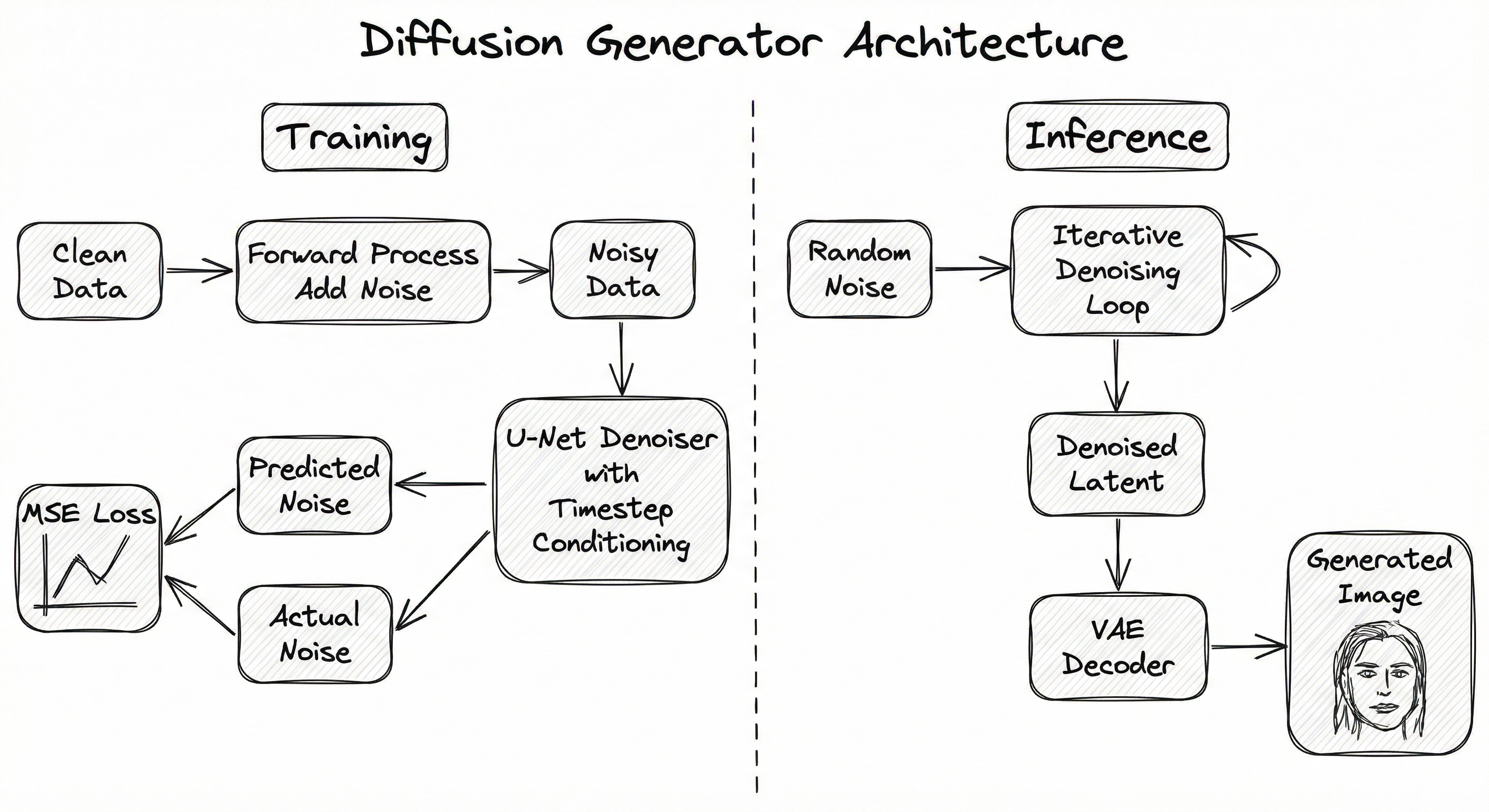
Two sections: Training and Inference. Training: Clean data flows through the forward process to create noisy data, which enters the U-Net denoiser (purple) along with timestep and conditioning inputs. The U-Net predicts noise, which is compared to actual noise in an MSE loss (red). Inference: Random noise enters an iterative denoising loop (purple) with conditioning, producing a denoised latent that passes through a VAE decoder (green) to produce the final generated image.
How to Implement
Implementation Approaches
There are four main paths to deploying diffusion generators in production:
Approach 1: Hugging Face Diffusers -- The most popular library for diffusion models. Provides pre-trained pipelines (Stable Diffusion, SDXL, ControlNet) and training utilities. Best for teams that want to fine-tune existing models or use them out-of-the-box. Minimal setup, strong community support.
Approach 2: Custom DDPM from Scratch -- For research or specialized data modalities (tabular, time series, molecular), implement the forward/reverse process and U-Net in PyTorch. Provides maximum control over architecture and training. Required when off-the-shelf image diffusion models don't apply to your data type.
Approach 3: TabDDPM for Tabular Data -- Purpose-built diffusion model for tabular synthetic data. Handles mixed data types (continuous + categorical) natively. Outperforms CTGAN and TVAE on most benchmarks. Use the tab-ddpm library from Yandex Research.
Approach 4: Commercial APIs -- DALL-E 3 via OpenAI API, Stability AI API, or Midjourney for image generation without managing infrastructure. Best for product teams that need synthetic images without ML engineering overhead.
Cost Considerations
Diffusion model training and inference costs vary dramatically by resolution and model size:
| Configuration | Training Cost | Inference Cost per Image | Hardware |
|---|---|---|---|
| DDPM 64x64 (from scratch) | $50-100 (~INR 4,200-8,400) | ~0.5s on GPU | 1x A100 for 2-3 days |
| Stable Diffusion fine-tune (LoRA) | $5-20 (~INR 420-1,680) | ~2s on GPU | 1x A100 for 2-4 hours |
| Stable Diffusion full fine-tune | $500-2,000 (~INR 42,000-1,68,000) | ~2s on GPU | 4-8x A100 for 3-5 days |
| SDXL inference only | N/A | ~4s on GPU | 1x A100 or 2x T4 |
| TabDDPM (tabular) | $2-10 (~INR 170-840) | ~5s for 10K rows | 1x T4 for 1-6 hours |
| DALL-E 3 API | N/A | $0.04-0.12 per image (~INR 3.4-10) | Cloud API |
Cost Tip: For Indian startups, fine-tuning with LoRA (Low-Rank Adaptation) on a single A100 instance from AWS Mumbai (ap-south-1) at ~$3.67/hr (~INR 308/hr) is the most cost-effective path to a custom diffusion model. A LoRA fine-tune of Stable Diffusion typically costs under ₹2,000 total.
import torch
import torch.nn as nn
import torch.nn.functional as F
from torch.utils.data import DataLoader
import math

# ─── Noise Schedule ──────────────────────────────────────────
class NoiseSchedule:
    """Linear or cosine noise schedule for DDPM."""
    def __init__(self, T=1000, schedule='cosine'):
        self.T = T
        if schedule == 'linear':
            self.betas = torch.linspace(1e-4, 0.02, T)
        elif schedule == 'cosine':
            steps = torch.arange(T + 1, dtype=torch.float64) / T
            alpha_bar = torch.cos((steps + 0.008) / 1.008 * math.pi / 2) ** 2
            alpha_bar = alpha_bar / alpha_bar[0]
            betas = 1 - alpha_bar[1:] / alpha_bar[:-1]
            self.betas = torch.clip(betas, 0.0001, 0.9999).float()

        self.alphas = 1.0 - self.betas
        self.alpha_bar = torch.cumprod(self.alphas, dim=0)
        self.sqrt_alpha_bar = torch.sqrt(self.alpha_bar)
        self.sqrt_one_minus_alpha_bar = torch.sqrt(1.0 - self.alpha_bar)

    def to(self, device):
        self.betas = self.betas.to(device)
        self.alphas = self.alphas.to(device)
        self.alpha_bar = self.alpha_bar.to(device)
        self.sqrt_alpha_bar = self.sqrt_alpha_bar.to(device)
        self.sqrt_one_minus_alpha_bar = self.sqrt_one_minus_alpha_bar.to(device)
        return self

# ─── Simplified U-Net (for illustration) ─────────────────────
class SimpleUNet(nn.Module):
    """Simplified U-Net for noise prediction. Production models use
    attention layers, residual blocks, and cross-attention for conditioning."""
    def __init__(self, in_channels=3, time_emb_dim=256):
        super().__init__()
        self.time_mlp = nn.Sequential(
            nn.Linear(1, time_emb_dim),
            nn.SiLU(),
            nn.Linear(time_emb_dim, time_emb_dim),
        )
        # Encoder
        self.enc1 = self._block(in_channels, 64)
        self.enc2 = self._block(64, 128)
        self.enc3 = self._block(128, 256)
        # Bottleneck
        self.bot = self._block(256, 512)
        # Decoder with skip connections
        self.dec3 = self._block(512 + 256, 256)
        self.dec2 = self._block(256 + 128, 128)
        self.dec1 = self._block(128 + 64, 64)
        self.out = nn.Conv2d(64, in_channels, 1)
        self.pool = nn.MaxPool2d(2)
        self.up = nn.Upsample(scale_factor=2, mode='bilinear', align_corners=True)

    def _block(self, in_ch, out_ch):
        return nn.Sequential(
            nn.Conv2d(in_ch, out_ch, 3, padding=1),
            nn.GroupNorm(8, out_ch),
            nn.SiLU(),
            nn.Conv2d(out_ch, out_ch, 3, padding=1),
            nn.GroupNorm(8, out_ch),
            nn.SiLU(),
        )

    def forward(self, x, t):
        # Time embedding (simplified)
        t_emb = self.time_mlp(t.unsqueeze(-1).float())
        # Encoder
        e1 = self.enc1(x)
        e2 = self.enc2(self.pool(e1))
        e3 = self.enc3(self.pool(e2))
        # Bottleneck
        b = self.bot(self.pool(e3))
        # Decoder
        d3 = self.dec3(torch.cat([self.up(b), e3], dim=1))
        d2 = self.dec2(torch.cat([self.up(d3), e2], dim=1))
        d1 = self.dec1(torch.cat([self.up(d2), e1], dim=1))
        return self.out(d1)

# ─── Training Loop ───────────────────────────────────────────
device = torch.device('cuda' if torch.cuda.is_available() else 'cpu')
model = SimpleUNet().to(device)
schedule = NoiseSchedule(T=1000, schedule='cosine').to(device)
optimizer = torch.optim.AdamW(model.parameters(), lr=2e-4)

for epoch in range(num_epochs):
    for images, _ in dataloader:
        images = images.to(device)  # [B, C, H, W] normalized to [-1, 1]
        batch_size = images.shape[0]

        # 1. Sample random timesteps
        t = torch.randint(0, schedule.T, (batch_size,), device=device)

        # 2. Sample noise
        epsilon = torch.randn_like(images)

        # 3. Create noisy images (forward process, closed form)
        sqrt_ab = schedule.sqrt_alpha_bar[t][:, None, None, None]
        sqrt_omab = schedule.sqrt_one_minus_alpha_bar[t][:, None, None, None]
        x_t = sqrt_ab * images + sqrt_omab * epsilon

        # 4. Predict noise
        epsilon_pred = model(x_t, t)

        # 5. Compute loss (simple MSE)
        loss = F.mse_loss(epsilon_pred, epsilon)

        # 6. Update
        optimizer.zero_grad()
        loss.backward()
        torch.nn.utils.clip_grad_norm_(model.parameters(), 1.0)
        optimizer.step()

print(f"Epoch {epoch}, Loss: {loss.item():.4f}")
This shows the complete DDPM training loop with a cosine noise schedule. Key points:
- The noise schedule precomputes and for efficient noisy sample creation via the reparameterization trick
- The forward process is computed in closed form (no iteration needed for training)
- The U-Net takes noisy input and timestep , predicts noise
- The loss is simply MSE between predicted and actual noise
- Gradient clipping (max norm 1.0) prevents training instabilities
- AdamW optimizer with learning rate 2e-4 is standard for diffusion models
For production, replace SimpleUNet with an attention-augmented U-Net (see Hugging Face Diffusers UNet2DModel).
import torch
import numpy as np

@torch.no_grad()
def ddpm_sample(model, schedule, shape, device):
    """Standard DDPM sampling (1000 steps)."""
    x = torch.randn(shape, device=device)  # Start from pure noise

    for t in reversed(range(schedule.T)):
        t_batch = torch.full((shape[0],), t, device=device, dtype=torch.long)

        # Predict noise
        epsilon_pred = model(x, t_batch)

        # Compute mean of p(x_{t-1} | x_t)
        alpha_t = schedule.alphas[t]
        alpha_bar_t = schedule.alpha_bar[t]
        beta_t = schedule.betas[t]

        mean = (1 / torch.sqrt(alpha_t)) * (
            x - (beta_t / torch.sqrt(1 - alpha_bar_t)) * epsilon_pred
        )

        # Add noise (except at t=0)
        if t > 0:
            noise = torch.randn_like(x)
            sigma = torch.sqrt(beta_t)
            x = mean + sigma * noise
        else:
            x = mean

    return x  # Generated samples in [-1, 1]


@torch.no_grad()
def ddim_sample(model, schedule, shape, device, num_steps=50, eta=0.0):
    """DDIM sampling with fewer steps. eta=0 gives deterministic sampling."""
    # Create sub-sequence of timesteps
    step_size = schedule.T // num_steps
    timesteps = list(range(0, schedule.T, step_size))
    timesteps = list(reversed(timesteps))

    x = torch.randn(shape, device=device)

    for i, t in enumerate(timesteps):
        t_batch = torch.full((shape[0],), t, device=device, dtype=torch.long)

        # Predict noise
        epsilon_pred = model(x, t_batch)

        alpha_bar_t = schedule.alpha_bar[t]

        # Get alpha_bar for previous timestep
        if i + 1 < len(timesteps):
            t_prev = timesteps[i + 1]
            alpha_bar_prev = schedule.alpha_bar[t_prev]
        else:
            alpha_bar_prev = torch.tensor(1.0, device=device)

        # Predicted x_0
        x0_pred = (x - torch.sqrt(1 - alpha_bar_t) * epsilon_pred) / torch.sqrt(alpha_bar_t)
        x0_pred = torch.clamp(x0_pred, -1, 1)  # Clip for stability

        # Direction pointing to x_t
        sigma = eta * torch.sqrt(
            (1 - alpha_bar_prev) / (1 - alpha_bar_t) * (1 - alpha_bar_t / alpha_bar_prev)
        )

        # DDIM update
        dir_xt = torch.sqrt(1 - alpha_bar_prev - sigma**2) * epsilon_pred
        noise = sigma * torch.randn_like(x) if eta > 0 else 0

        x = torch.sqrt(alpha_bar_prev) * x0_pred + dir_xt + noise

    return x

# Generate samples
samples_ddpm = ddpm_sample(model, schedule, (16, 3, 64, 64), device)  # ~60 seconds
samples_ddim = ddim_sample(model, schedule, (16, 3, 64, 64), device, num_steps=50)  # ~3 seconds
Two sampling methods compared:
- DDPM sampling: Full 1000-step stochastic reverse process. Highest quality but slow (~60s per batch on GPU).
- DDIM sampling: Deterministic (
eta=0) or stochastic (eta>0) with arbitrary step count. 50 steps gives near-DDPM quality at 20x speedup. Settingeta=0makes generation deterministic -- same noise input always produces the same output, useful for reproducibility.
The key DDIM insight is that the DDPM reverse process can be viewed as discretizing a continuous ODE, and we can solve it with larger step sizes. The x0_pred clipping to [-1, 1] prevents prediction artifacts from accumulating across steps.
from diffusers import StableDiffusionPipeline, DDPMScheduler
from diffusers.training_utils import compute_snr_weights
from peft import LoraConfig
import torch
from torch.utils.data import Dataset, DataLoader
from torchvision import transforms
from PIL import Image
import os

# Load pre-trained Stable Diffusion
model_id = "stabilityai/stable-diffusion-2-1-base"
pipeline = StableDiffusionPipeline.from_pretrained(
    model_id, torch_dtype=torch.float16
)
pipeline.to("cuda")

# Configure LoRA for efficient fine-tuning
lora_config = LoraConfig(
    r=8,                     # LoRA rank (4-16 typical)
    lora_alpha=32,           # Scaling factor
    target_modules=["to_q", "to_v", "to_k", "to_out.0"],  # Attention layers
    lora_dropout=0.05,
)

# Apply LoRA to U-Net
pipeline.unet.add_adapter(lora_config)

# Custom dataset
class SyntheticDataset(Dataset):
    def __init__(self, image_dir, captions, transform=None):
        self.image_dir = image_dir
        self.captions = captions
        self.transform = transform or transforms.Compose([
            transforms.Resize(512),
            transforms.CenterCrop(512),
            transforms.ToTensor(),
            transforms.Normalize([0.5], [0.5]),
        ])

    def __len__(self):
        return len(self.captions)

    def __getitem__(self, idx):
        image = Image.open(os.path.join(self.image_dir, f"{idx}.png"))
        image = self.transform(image)
        caption = self.captions[idx]
        return image, caption

# Training setup
optimizer = torch.optim.AdamW(
    pipeline.unet.parameters(),
    lr=1e-4,
    weight_decay=1e-2
)
noise_scheduler = DDPMScheduler.from_pretrained(model_id, subfolder="scheduler")

# Fine-tuning loop (simplified)
for epoch in range(num_epochs):
    for images, captions in dataloader:
        images = images.to("cuda", dtype=torch.float16)

        # Encode images to latent space
        latents = pipeline.vae.encode(images).latent_dist.sample()
        latents = latents * pipeline.vae.config.scaling_factor

        # Encode text prompts
        text_inputs = pipeline.tokenizer(
            captions, padding="max_length", max_length=77,
            truncation=True, return_tensors="pt"
        ).to("cuda")
        text_embeddings = pipeline.text_encoder(text_inputs.input_ids)[0]

        # Sample noise and timesteps
        noise = torch.randn_like(latents)
        timesteps = torch.randint(
            0, noise_scheduler.config.num_train_timesteps,
            (latents.shape[0],), device="cuda"
        )

        # Add noise to latents
        noisy_latents = noise_scheduler.add_noise(latents, noise, timesteps)

        # Predict noise
        noise_pred = pipeline.unet(
            noisy_latents, timesteps, encoder_hidden_states=text_embeddings
        ).sample

        # MSE loss
        loss = torch.nn.functional.mse_loss(noise_pred, noise)

        optimizer.zero_grad()
        loss.backward()
        optimizer.step()

# Save LoRA weights (~10-50 MB vs 2GB for full model)
pipeline.unet.save_pretrained("./lora-weights")

# Inference with fine-tuned model
pipeline.unet.load_adapter("./lora-weights")
image = pipeline("A product photo in the style of my brand", num_inference_steps=30).images[0]
LoRA fine-tuning is the most practical approach for customizing Stable Diffusion:
- LoRA rank of 8 adds only ~4M trainable parameters vs 860M in the full U-Net
- Target modules are the attention layers (
to_q,to_v,to_k,to_out) where most task-specific knowledge is captured - Weight savings: LoRA checkpoint is 10-50 MB vs 2+ GB for full model
- Training time: 500-2000 steps on 100-500 images, typically 1-4 hours on a single A100
- Latent encoding: Images are compressed via the VAE before diffusion training, reducing the spatial compute by 64x
This approach is widely used by Indian e-commerce companies (Flipkart, Myntra, Meesho) for generating product images in specific styles.
import numpy as np
import pandas as pd
from tab_ddpm import GaussianMultinomialDiffusion
from tab_ddpm.modules import MLPDiffusion
import torch

# Load and prepare tabular data
df = pd.read_csv('customer_transactions.csv')

# Separate numerical and categorical columns
num_cols = ['age', 'income', 'transaction_amount', 'account_balance']
cat_cols = ['gender', 'city', 'product_category', 'payment_method']

# Preprocess: normalize numerical, encode categorical
from sklearn.preprocessing import StandardScaler, OrdinalEncoder

scaler = StandardScaler()
X_num = scaler.fit_transform(df[num_cols].values).astype(np.float32)

encoder = OrdinalEncoder()
X_cat = encoder.fit_transform(df[cat_cols].values).astype(np.int64)

# Get cardinalities for each categorical column
num_categories = [int(df[col].nunique()) for col in cat_cols]

# Configure TabDDPM
model = MLPDiffusion(
    d_in=len(num_cols),             # Number of numerical features
    num_classes=num_categories,      # Cardinalities of categorical features
    is_y_cond=False,                 # Unconditional generation
    d_layers=[256, 256, 256],        # MLP hidden layers
    dropout=0.0,
    dim_t=128,                       # Timestep embedding dimension
)

diffusion = GaussianMultinomialDiffusion(
    num_classes=np.array(num_categories),
    num_numerical_features=len(num_cols),
    denoise_fn=model,
    gaussian_loss_type='mse',
    num_timesteps=1000,
    scheduler='cosine',
    device=torch.device('cuda'),
)

# Training
X_num_tensor = torch.tensor(X_num, device='cuda')
X_cat_tensor = torch.tensor(X_cat, device='cuda')

optimizer = torch.optim.Adam(diffusion.parameters(), lr=1e-3, weight_decay=1e-5)

for epoch in range(1000):
    # Random batch
    idx = np.random.choice(len(X_num), size=256, replace=False)
    x_num = X_num_tensor[idx]
    x_cat = X_cat_tensor[idx]

    loss = diffusion.mixed_loss(x_num, x_cat)

    optimizer.zero_grad()
    loss.backward()
    optimizer.step()

    if epoch % 100 == 0:
        print(f"Epoch {epoch}, Loss: {loss.item():.4f}")

# Generate synthetic data
with torch.no_grad():
    x_num_syn, x_cat_syn = diffusion.sample(num_samples=10000)

# Inverse transform back to original scale
X_num_syn = scaler.inverse_transform(x_num_syn.cpu().numpy())
X_cat_syn = encoder.inverse_transform(x_cat_syn.cpu().numpy())

# Combine into DataFrame
synthetic_df = pd.DataFrame(
    np.hstack([X_num_syn, X_cat_syn]),
    columns=num_cols + cat_cols
)
print(f"Generated {len(synthetic_df)} synthetic rows")
print(synthetic_df.describe())
TabDDPM extends diffusion models to tabular data by handling mixed types:
- Numerical features: Standard Gaussian diffusion (add/remove Gaussian noise)
- Categorical features: Multinomial diffusion (corrupt by randomly replacing categories, then denoise by predicting the original category)
- Mixed loss: Combines Gaussian MSE loss for numerical columns and cross-entropy loss for categorical columns
- MLP denoiser: Uses an MLP instead of U-Net since tabular data has no spatial structure
TabDDPM outperforms CTGAN on most tabular benchmarks (ICML 2023) and is particularly strong for datasets with complex multivariate dependencies. It also provides better privacy properties than GAN-based methods because the diffusion process naturally adds noise that obscures individual data points.
# Stable Diffusion LoRA Fine-Tuning Config (YAML)
model:
  base_model: stabilityai/stable-diffusion-2-1-base
  resolution: 512
  dtype: float16

lora:
  rank: 8
  alpha: 32
  target_modules:
    - to_q
    - to_v
    - to_k
    - to_out.0
  dropout: 0.05

training:
  num_epochs: 100
  batch_size: 4
  gradient_accumulation_steps: 4  # effective batch size = 16
  learning_rate: 1e-4
  lr_scheduler: cosine
  warmup_steps: 100
  optimizer: adamw
  weight_decay: 0.01
  max_grad_norm: 1.0
  mixed_precision: fp16
  ema_decay: 0.9999

noise_schedule:
  type: cosine
  num_timesteps: 1000
  prediction_type: epsilon  # or v_prediction

guidance:
  classifier_free: true
  uncond_prob: 0.1  # 10% unconditional dropout
  guidance_scale: 7.5  # inference only

data:
  train_dir: ./data/train
  caption_column: text
  image_column: image
  augmentation:
    - random_flip
    - center_crop

inference:
  scheduler: ddim
  num_steps: 30
  guidance_scale: 7.5
  negative_prompt: "blurry, low quality, distorted"
Common Implementation Mistakes
- ●
Using too few diffusion steps at training time: Setting degrades quality significantly because the model doesn't learn the full spectrum of noise levels. Always train with (DDPM standard). You can use fewer steps at inference time with DDIM or DPM-Solver, but training should use the full schedule.
- ●
Forgetting to normalize data to [-1, 1]: The forward process assumes data starts near zero. If images are in [0, 255] range, the noise schedule parameters are meaningless. Always normalize:
x = 2 * (x / 255) - 1. For tabular data, use StandardScaler to center and scale features. - ●
Setting classifier-free guidance scale too high: Guidance scale often produces oversaturated, artifact-ridden images. The optimal range is typically 5-10 for text-to-image. Always sweep on a validation set before deploying. Too-low (< 3) produces diverse but unfaithful outputs; too-high produces faithful but homogeneous outputs.
- ●
Not clipping predicted during DDIM sampling: When using the predicted- formulation, the prediction can drift outside [-1, 1], causing cascading errors in subsequent steps. Always clip:
x0_pred = torch.clamp(x0_pred, -1, 1). This is a subtle bug that manifests as blown-out highlights or color artifacts in generated images. - ●
Mixing up noise prediction (-prediction) and sample prediction (-prediction): Different diffusion model implementations use different parameterizations. Stable Diffusion 1.x uses -prediction. Some newer models use -prediction (velocity parameterization). Using the wrong prediction target with the wrong sampler produces garbage. Always check the model card.
- ●
Ignoring EMA (Exponential Moving Average): Production diffusion models use EMA of model weights for inference (typically decay 0.9999). Training without EMA results in noticeably lower sample quality. The EMA model smooths out noisy gradient updates and produces sharper, more consistent samples.
When Should You Use This?
Use When
You need high-fidelity synthetic data that matches or exceeds GAN quality -- diffusion models consistently achieve state-of-the-art FID scores across image, audio, and tabular modalities
Training stability is important and you cannot afford the trial-and-error of GAN hyperparameter tuning -- diffusion models train with a simple MSE loss with no adversarial dynamics
You need controllable generation via text prompts, class labels, or other conditioning -- classifier-free guidance provides a principled, tunable mechanism for conditional generation
You're working with tabular data and need synthetic datasets that preserve complex multivariate relationships -- TabDDPM outperforms CTGAN/TVAE on most benchmarks
You need full mode coverage -- diffusion models don't suffer from mode collapse, making them suitable for generating diverse synthetic datasets that represent the full data distribution
Your application can tolerate multi-second inference times (e.g., batch data generation, offline augmentation, non-real-time content creation)
You want to fine-tune a pre-trained model for a custom domain -- LoRA and DreamBooth enable efficient adaptation of Stable Diffusion with as few as 5-20 images
Avoid When
You need real-time generation (< 100ms per sample) -- even with DDIM acceleration, diffusion models require 15-50 denoising steps per sample, taking 1-10 seconds on GPU. Use GANs (single forward pass) for real-time applications
Your compute budget is very limited and you cannot afford GPU time for training or inference -- diffusion model training requires at least one modern GPU (T4/A100) for several hours, and inference is 100-1000x slower than GANs per sample
You're working with discrete sequences (text, code) where autoregressive models (GPT, LLaMA) are the natural fit -- while discrete diffusion models exist, they remain inferior to autoregressive approaches for text generation
You need a simple, interpretable generative model -- the iterative denoising process with 1000 timesteps and noise schedules adds complexity that may be unnecessary for simple data distributions. Consider a VAE or statistical copula instead
Your dataset is extremely small (< 100 samples) -- diffusion models, like all deep generative models, need sufficient data to learn the distribution. For tiny datasets, use classical augmentation (flips, rotations) or few-shot techniques
You need exact density estimation for anomaly detection or out-of-distribution detection -- while diffusion models can estimate likelihoods via the ELBO, this is computationally expensive and normalizing flows or VAEs are more natural choices
Key Tradeoffs
Core Tradeoff: Quality vs. Inference Speed
The fundamental tradeoff of diffusion models is their iterative sampling process. More denoising steps produce higher-quality samples but take proportionally longer. Here's how the tradeoff manifests:
| Sampler | Steps | Quality (FID) | Time per Image (A100) | Use Case |
|---|---|---|---|---|
| DDPM | 1000 | Best (~2.0) | ~60s | Research, gold-standard quality |
| DDIM | 50 | Very Good (~3.5) | ~3s | Production batch generation |
| DPM-Solver++ | 20 | Good (~4.5) | ~1.5s | Low-latency production |
| LCM (distilled) | 4 | Acceptable (~8.0) | ~0.3s | Near-real-time applications |
Diffusion vs. GAN vs. VAE
| Dimension | Diffusion Model | GAN | VAE |
|---|---|---|---|
| Sample Quality | Best (FID ~2) | Excellent (FID ~3) | Good (blurry) |
| Training Stability | Excellent (MSE loss) | Poor (mode collapse) | Excellent (ELBO) |
| Mode Coverage | Full | Partial (mode collapse) | Full |
| Inference Speed | Slow (1-60s) | Fast (<50ms) | Fast (<50ms) |
| Controllability | Excellent (CFG) | Limited (cGAN) | Moderate (latent) |
| Density Estimation | Via ELBO (expensive) | No | Yes (direct) |
| Training Cost (64x64) | $50-100 | $10-50 | $5-20 |
Latent vs. Pixel-Space Diffusion
Latent diffusion (Stable Diffusion) operates on compressed representations, reducing compute by ~64x. The tradeoff: a small loss in fine-grained detail due to VAE compression. For most applications, this is negligible and overwhelmingly worth the speed improvement.
| Aspect | Pixel-Space DDPM | Latent Diffusion |
|---|---|---|
| Resolution | Up to 256x256 practical | 512x512 to 2048x2048 |
| VRAM (training) | 24-80 GB | 8-24 GB |
| Training Time | Days-weeks | Hours-days |
| Detail Fidelity | Highest | Very high (slight VAE loss) |
| Consumer GPU Feasible | 64x64 only | Yes (512x512 on RTX 3090) |
Practitioner's Note: For 95% of production use cases in India, latent diffusion with DDIM sampling (30-50 steps) is the right choice. It runs on a single A100 or even an RTX 4090 (₹1.6 lakh), generates 512x512 images in ~2 seconds, and achieves near-DDPM quality. Reserve pixel-space DDPM for research or when you need absolute maximum quality at low resolutions.
Alternatives & Comparisons
GANs generate samples in a single forward pass (~50ms), making them 100-1000x faster than diffusion models at inference. However, GANs suffer from mode collapse, training instability, and require careful hyperparameter tuning. Diffusion models achieve better or equivalent sample quality with far more stable training. Choose GANs when real-time generation is required (interactive applications, video synthesis). Choose diffusion models when sample quality, diversity, and training reliability matter more than inference speed.
VAEs provide explicit density estimation , stable training, and fast single-pass generation. However, VAE samples tend to be blurry due to the Gaussian assumption and pixel-wise reconstruction loss. Diffusion models produce dramatically sharper samples. Choose VAEs when you need density estimation (anomaly detection), fast inference, or are working with very small datasets. Choose diffusion models when sample quality is the priority and you can afford iterative sampling.
CTGAN is a GAN-based approach specifically designed for tabular synthetic data. While CTGAN handles mixed data types well, TabDDPM (diffusion-based) consistently outperforms it on tabular benchmarks (ICML 2023). CTGAN trains faster and generates samples faster, but TabDDPM produces higher-fidelity synthetic data with better privacy properties. Choose CTGAN when inference speed matters for tabular data. Choose TabDDPM/diffusion when tabular data quality is the priority.
Pros, Cons & Tradeoffs
Advantages
State-of-the-art sample quality: Diffusion models achieve the best FID scores across image generation benchmarks, producing samples that are indistinguishable from real data. Stable Diffusion generates photorealistic 512x512 images; TabDDPM produces synthetic tables that preserve complex multivariate correlations.
Extremely stable training: The MSE noise prediction objective is a simple, well-behaved loss function. No adversarial dynamics, no mode collapse, no careful balancing of competing networks. If you can train a standard regression model, you can train a diffusion model.
Full mode coverage and diversity: Unlike GANs, diffusion models don't suffer from mode collapse. The forward process covers the entire data distribution, and the reverse process must learn to reconstruct all modes. This makes them ideal for generating diverse synthetic datasets.
Powerful controllability via classifier-free guidance: Text-to-image, class-conditional, layout-guided, and inpainting are all supported through a single, principled conditioning mechanism. The guidance scale provides a smooth knob for the fidelity-diversity tradeoff.
Rich pre-trained model ecosystem: Stable Diffusion, SDXL, and hundreds of community fine-tunes are freely available. LoRA fine-tuning enables domain adaptation with as few as 5-20 images and ₹2,000 in compute. No other generative model family has this breadth of pre-trained models.
Mathematically principled: Grounded in variational inference, score matching, and stochastic differential equations. The theory provides clear insights into why things work and how to improve them, unlike the empirical nature of GAN training tricks.
Modality-agnostic: The same framework applies to images, audio, video, 3D shapes, molecular structures, tabular data, and time series. Only the denoiser architecture and data preprocessing change.
Disadvantages
Slow inference: Generating a single sample requires 15-1000 denoising steps, each involving a full neural network forward pass. Even with acceleration (DDIM, DPM-Solver), inference is 100-1000x slower than GANs. A 512x512 Stable Diffusion image takes ~2 seconds on an A100 vs ~50ms for a GAN.
High VRAM requirements: The U-Net denoiser for Stable Diffusion requires 4-8 GB VRAM at float16. SDXL needs 8-16 GB. Fine-tuning requires 16-24 GB. This limits deployment to GPU-equipped servers, making edge deployment challenging without distillation.
Computationally expensive training: Training a diffusion model from scratch requires significant GPU hours. A custom 256x256 DDPM takes 2-5 days on an A100 (~$300-750 / INR 25,000-63,000). Pre-trained models and LoRA fine-tuning mitigate this, but cold-start training remains expensive.
Classifier-free guidance doubles inference cost: Each denoising step requires two U-Net forward passes (one conditional, one unconditional). This doubles the already-slow inference time. Techniques like guidance distillation help but add training complexity.
Noise schedule sensitivity: Sample quality is sensitive to the noise schedule. A poorly chosen schedule wastes compute on uninformative timesteps or corrupts data too aggressively. While cosine schedules work well as defaults, optimal schedules are data-dependent and require experimentation.
Evaluation is challenging: FID, IS, and CLIP scores are the standard metrics, but they don't always correlate with human perception. Evaluating tabular diffusion quality requires domain-specific statistical tests. There is no single universally accepted quality metric.
Failure Modes & Debugging
Noise schedule mismatch
Cause
Using a noise schedule designed for one data modality or resolution on a different one. For example, a linear schedule tuned for 256x256 images applied to 64x64 images, or an image noise schedule applied to tabular data. The schedule determines how much signal remains at each timestep -- get it wrong and the model either can't learn (too aggressive) or wastes compute (too conservative).
Symptoms
Generated samples are either completely noisy (schedule too aggressive -- data is destroyed before the model can learn intermediate states) or overly smooth/blurry (schedule too conservative -- the model never learns to generate fine details from high noise levels). Training loss may converge but sample quality remains poor. FID scores plateau at unacceptably high levels.
Mitigation
Start with the cosine schedule as default (it's more robust than linear across resolutions). For custom data modalities, visualize the noised samples at various timesteps: at , you should see a mixture of recognizable structure and significant noise. If the data is fully destroyed by , the schedule is too aggressive. If it's still mostly clean at , it's too conservative. For tabular data, TabDDPM's default cosine schedule with works well without modification.
Guidance scale collapse
Cause
Setting the classifier-free guidance scale too high (> 15-20) during inference. High guidance scales amplify the conditional signal but also amplify prediction errors, causing the denoising process to diverge from the natural data manifold.
Symptoms
Generated images become oversaturated, with blown-out colors, unnatural contrast, and repeated patterns or textures. Fine details are lost, and images look "deep-fried" or oversharpened. At extreme scales (), outputs may contain visible artifacts or become completely incoherent.
Mitigation
Start with (the Stable Diffusion default) and sweep from 3.0 to 12.0 on a validation set. Use dynamic thresholding (Imagen) to clip predictions during sampling, preventing the divergence that high guidance scales cause. For class-conditional generation, lower scales () are typically sufficient. Monitor the distribution of predicted noise values -- they should not systematically exceed the training distribution.
VAE bottleneck in latent diffusion
Cause
The pretrained VAE's compression is too lossy for the target domain. The VAE was trained on natural images but is being used for medical scans, satellite imagery, or other specialized domains where fine details matter. The diffusion model generates perfect latents, but the VAE decoder cannot reconstruct domain-specific details.
Symptoms
Generated images look reasonable at a glance but lack domain-specific fine details. Medical images may lose subtle lesion textures. Satellite images may lack building edge precision. Text in generated images is consistently illegible (a common Stable Diffusion failure). The diffusion model's training loss converges normally, making this failure easy to miss.
Mitigation
Fine-tune the VAE decoder on domain-specific data (Stable Diffusion's VAE is only 83M parameters -- fine-tuning is cheap). Alternatively, use a higher-resolution VAE latent space (less compression). For text rendering, consider pixel-space diffusion or specialized text-aware architectures. Always evaluate end-to-end sample quality (after VAE decoding), not just latent-space metrics.
Memorization and privacy leakage
Cause
Training on a small dataset or training for too many epochs causes the diffusion model to memorize training samples rather than learning the underlying distribution. Generated samples are near-copies of training data, defeating the purpose of synthetic data generation and potentially violating privacy.
Symptoms
Nearest-neighbor analysis shows generated samples with very high similarity (cosine similarity > 0.95) to specific training examples. FID scores may look good (because memorized samples are realistic) but diversity metrics (recall, coverage) are poor. Privacy audits (membership inference attacks) succeed at rates significantly above chance.
Mitigation
Monitor training data memorization using nearest-neighbor distance metrics throughout training. Apply early stopping based on FID or diversity metrics, not just training loss. For privacy-critical applications, use differentially private diffusion (DP-Diffusion) which adds calibrated noise to gradients during training. Limit training epochs: for LoRA fine-tuning on < 500 images, 50-100 epochs is typically sufficient. For TabDDPM, Kotelnikov et al. (2023) show that diffusion models have inherently better privacy properties than GANs, but explicit DP guarantees still require DP-SGD.
Timestep embedding failure
Cause
Incorrect implementation of the timestep embedding causes the U-Net to ignore or misinterpret the noise level. Common causes: timestep not normalized to [0, 1] before sinusoidal encoding, timestep embedding not injected into all residual blocks, or using integer timesteps when the model expects continuous values.
Symptoms
The model predicts the same noise pattern regardless of timestep, or predictions at low noise levels are as noisy as predictions at high noise levels. Training loss may still decrease (the model learns an average denoising function) but sample quality is poor. Visual inspection of intermediate denoising steps shows erratic behavior -- the sample doesn't progressively clean up but jumps between noisy and partially denoised states.
Mitigation
Use the standard sinusoidal timestep embedding from the original Transformer paper: . Verify that the embedding is injected into every residual block of the U-Net (typically via addition after a linear projection). Test by checking that the model's predictions change smoothly as varies from 0 to for a fixed input. When using pre-trained models, always match the timestep normalization convention (integer vs. continuous, 0-indexed vs. 1-indexed).
Distribution shift in tabular diffusion
Cause
For TabDDPM and other tabular diffusion models, incorrect preprocessing (not centering/scaling numerical features, not handling missing values, or using label encoding instead of ordinal encoding for ordered categories) causes the Gaussian forward process to operate on data with unexpected statistics.
Symptoms
Generated numerical features have incorrect ranges (e.g., negative ages, incomes in the billions). Categorical features have unrealistic joint distributions. Statistical tests (Kolmogorov-Smirnov, chi-squared) show significant divergence between real and synthetic marginals. Downstream models trained on synthetic data perform significantly worse than those trained on real data.
Mitigation
Always standardize numerical features (zero mean, unit variance) before diffusion training. Use ordinal encoding for ordered categories and one-hot-like multinomial diffusion for unordered categories. Handle missing values explicitly (either impute before training or use a dedicated missing-value token). After generation, apply inverse transformations and clip to valid ranges. Run column-level and pairwise statistical validation before using synthetic data downstream.
Placement in an ML System
Where Does It Sit in the Pipeline?
Diffusion generators sit at the data preparation stage of ML pipelines, generating synthetic training data, augmenting limited real datasets, or creating test data for downstream models.
Synthetic Data Generation Pipeline: Raw Data -> Data Validation -> Diffusion Generator -> Synthetic Data Validation -> Merge with Real Data -> Feature Engineering -> Model Training
The diffusion generator receives validated real data as its training input and produces synthetic samples that are validated for quality before being mixed with real data for downstream model training.
Key Integration Points:
-
Data validation (upstream): Real data must be clean and properly formatted before training the diffusion model. Garbage in, garbage out applies doubly for generative models.
-
Synthetic data validation (downstream): Generated data must pass quality checks before use. These include statistical tests (KS test, chi-squared), downstream model performance comparison, and privacy audits (nearest-neighbor distance, membership inference).
-
Feature store: The diffusion generator may read feature definitions and constraints from the feature store to ensure synthetic data respects domain constraints (e.g., age > 0, email format, valid pin codes).
Production Pattern: In practice, diffusion generators run as batch jobs (not real-time services). A nightly or weekly cron job generates synthetic data, validates it, and uploads it to the data warehouse. The ML training pipeline then reads from this warehouse. This decouples generation latency from training latency.
Pipeline Stage
Data Generation / Augmentation
Upstream
- Training Dataset
- Feature Store
- Data Validation
Downstream
- Data Validation
- Feature Engineering
- Model Training
- Evaluation Pipeline
Scaling Bottlenecks
The iterative sampling process is the dominant bottleneck. Generating 100K synthetic images at 512x512 with Stable Diffusion (30 DDIM steps) requires 56 GPU-hours on an A100 (2,000 / INR 1,68,000).
Mitigation strategies:
- Batch parallelism: Run multiple samples per GPU (batch size 4-8 depending on VRAM)
- Multi-GPU: Distribute batches across GPUs (embarrassingly parallel)
- Distilled samplers: LCM (Latent Consistency Models) reduce steps from 30 to 4, giving ~7.5x speedup
- Quantization: INT8 U-Net inference reduces VRAM by 50% and increases throughput by ~30%
Large-scale synthetic data generation produces enormous datasets. 1M images at 512x512 PNG requires ~1.5 TB of storage. Use JPEG compression (quality 95) to reduce to ~200 GB with minimal quality loss. For tabular data, storage is rarely a concern.
Full fine-tuning of Stable Diffusion's U-Net (860M parameters) requires 24-40 GB VRAM. LoRA reduces this to 8-16 GB. Training from scratch on custom data requires 40-80 GB VRAM per GPU.
Production Case Studies
Stability AI released Stable Diffusion as an open-source latent diffusion model trained on LAION-5B. The model democratized high-quality image generation by running on consumer GPUs (RTX 3060 with 8GB VRAM). The latent diffusion architecture reduced compute requirements by ~64x compared to pixel-space diffusion, making 512x512 generation feasible on hardware costing ₹30,000-50,000.
Within 6 months of release, Stable Diffusion was downloaded over 10 million times. It spawned an ecosystem of 100,000+ community fine-tunes on Civitai and Hugging Face. The model generates a 512x512 image in ~2 seconds on an RTX 3090, compared to ~60 seconds for pixel-space DDPM at the same resolution.
Google's Imagen demonstrated that scaling the text encoder (T5-XXL, 11B parameters) was more effective than scaling the diffusion model itself for text-to-image quality. Imagen achieved a new state-of-the-art FID of 7.27 on COCO (zero-shot) and introduced dynamic thresholding to prevent color saturation at high classifier-free guidance scales. The cascaded architecture (64x64 base + two super-resolution diffusion models) produces 1024x1024 images.
Imagen achieved a human preference rate of 39.2% over competing models (including DALL-E 2) in side-by-side comparisons. The paper demonstrated that diffusion models + large language model encoders could produce photorealistic images with unprecedented text alignment.
Yandex Research developed TabDDPM, applying the diffusion framework to tabular synthetic data generation. They introduced Gaussian diffusion for numerical features and multinomial diffusion for categorical features, trained jointly with a single MLP denoiser. TabDDPM was evaluated on 15 tabular datasets against CTGAN, TVAE, and other baselines.
TabDDPM outperformed GAN and VAE baselines on 11 of 15 datasets for downstream ML utility (training a classifier on synthetic data and evaluating on real test data). It also showed superior privacy properties, with synthetic samples being less similar to training data than CTGAN-generated samples. Published at ICML 2023.
Flipkart's computer vision team has explored diffusion-based approaches for product image generation and enhancement. Using fine-tuned Stable Diffusion models (via LoRA and ControlNet), the team generates catalog images with consistent backgrounds, lighting, and angles for products uploaded by sellers with poor photography. This improves the visual consistency of the marketplace, which directly impacts click-through rates and conversion.
Synthetic product image pipelines reduced the time for catalog image processing from 2-3 days (manual photography/editing) to minutes. A/B tests showed that AI-enhanced product images improved click-through rates by 8-15% for categories with traditionally poor seller imagery (fashion accessories, home decor).
Tooling & Ecosystem
The de facto standard library for diffusion models. Provides pre-trained pipelines (Stable Diffusion, SDXL, ControlNet, Kandinsky), training scripts, 20+ schedulers (DDPM, DDIM, DPM-Solver, Euler, LCM), and LoRA/DreamBooth fine-tuning utilities. Supports PyTorch and JAX/Flax.
Feature-rich web interface for Stable Diffusion with support for txt2img, img2img, inpainting, outpainting, LoRA loading, ControlNet, and batch generation. Widely used for interactive experimentation and small-scale production. Runs on consumer GPUs.
Node-based visual workflow editor for diffusion model pipelines. Enables complex generation workflows (multi-model, multi-ControlNet, upscaling chains) without code. More flexible than AUTOMATIC1111 for production pipelines. Supports SDXL, SVD, and custom nodes.
Official implementation of TabDDPM for tabular synthetic data generation. Supports mixed numerical and categorical features with Gaussian and multinomial diffusion respectively. Includes training scripts, evaluation metrics, and benchmark comparisons. Published at ICML 2023.
Cloud API for Stable Diffusion and SDXL generation without managing infrastructure. Pricing starts at $0.002-0.006 per image (~INR 0.17-0.50). Supports text-to-image, image-to-image, inpainting, and upscaling. Best for product teams that need synthetic images without GPU management.
OpenAI's diffusion-based image generation API. Tight integration with ChatGPT for prompt refinement. Pricing: $0.04-0.12 per image (~INR 3.4-10) depending on resolution. Best text-to-image alignment among commercial APIs. No self-hosting option.
Research & References
Ho, Jain & Abbeel (2020)NeurIPS 2020
The foundational DDPM paper that demonstrated diffusion models could match GAN quality on image generation. Introduced the simplified noise-prediction training objective and showed state-of-the-art FID scores on CIFAR-10 and LSUN.
Rombach, Blattmann, Lorenz, Esser & Ommer (2022)CVPR 2022
Introduced latent diffusion models (LDMs) that operate in a compressed VAE latent space, reducing compute by ~64x. This architecture became Stable Diffusion, democratizing high-resolution image generation on consumer hardware.
Ho & Salimans (2022)NeurIPS 2022 Workshop
Proposed jointly training conditional and unconditional diffusion models by randomly dropping the conditioning signal, then combining the score estimates at inference. This eliminated the need for a separate classifier while providing controllable conditioning strength via the guidance scale .
Song, Meng & Ermon (2021)ICLR 2021
Introduced DDIM, a non-Markovian reverse process enabling deterministic sampling with 10-50x fewer steps than DDPM. DDIM also enables latent space interpolation and consistent image editing through its deterministic mapping between noise and data.
Song, Sohl-Dickstein, Kingma, Kumar, Ermon & Poole (2021)ICLR 2021 (Oral)
Unified diffusion probabilistic models and score-based generative models through the lens of stochastic differential equations (SDEs). Showed that both frameworks are discretizations of the same continuous-time process, enabling new sampler designs and exact likelihood computation.
Kotelnikov, Baranchuk, Rubachev & Babenko (2023)ICML 2023
Extended diffusion models to tabular data using Gaussian diffusion for numerical features and multinomial diffusion for categorical features. Outperformed CTGAN and TVAE on 11 of 15 benchmarks for downstream ML utility, with superior privacy properties.
Nichol & Dhariwal (2021)ICML 2021
Introduced the cosine noise schedule (more gradual than linear, better image quality), learned variance prediction, and importance sampling for the training objective. These improvements matched or exceeded state-of-the-art log-likelihoods while maintaining high sample quality.
Dhariwal & Nichol (2021)NeurIPS 2021
Demonstrated that diffusion models with classifier guidance achieve a new state-of-the-art FID of 2.97 on ImageNet 256x256, surpassing BigGAN-deep. Introduced architectural improvements (adaptive group normalization, multi-head attention at multiple resolutions) that became standard in subsequent work.
Interview & Evaluation Perspective
Common Interview Questions
- ●
Explain the forward and reverse process in a diffusion model. Why does this decomposition make training easier than GANs?
- ●
What is classifier-free guidance? How does it work, and why is it preferred over classifier guidance?
- ●
Compare diffusion models with GANs and VAEs. When would you choose each?
- ●
What is latent diffusion, and why is it important for high-resolution image generation?
- ●
How would you use diffusion models to generate synthetic tabular data for a privacy-sensitive application?
- ●
Explain the noise schedule in DDPM. What happens if you choose a bad schedule?
- ●
How do you accelerate diffusion model inference? Compare DDIM, DPM-Solver, and distillation approaches.
- ●
Design a synthetic data generation pipeline using diffusion models for an e-commerce platform with 10M product images.
Key Points to Mention
- ●
The forward process is fixed and parameter-free (just adding Gaussian noise); only the reverse process is learned. This decomposition converts the hard problem of generation into many easy denoising subproblems.
- ●
The training objective is a simple MSE loss between predicted and actual noise -- no adversarial dynamics, no mode collapse. This is why diffusion models scale reliably to larger models and datasets.
- ●
Classifier-free guidance trains a single model that works both conditionally and unconditionally by randomly dropping the conditioning signal. At inference, the guidance scale provides a smooth tradeoff between conditioning fidelity and sample diversity.
- ●
Latent diffusion (Stable Diffusion) reduces compute by ~64x by operating in a compressed VAE latent space. This is what made high-resolution generation practical on consumer hardware.
- ●
For tabular data, TabDDPM uses Gaussian diffusion for numerical and multinomial diffusion for categorical features, outperforming CTGAN on most benchmarks (ICML 2023).
- ●
Inference acceleration comes in three flavors: better samplers (DDIM, DPM-Solver for 20-50 steps), distillation (LCM for 1-4 steps), and model compression (quantization, pruning). These are complementary and can be combined.
Pitfalls to Avoid
- ●
Claiming diffusion models are "slow" without qualifying that this applies to inference, not training. Training stability is actually a major advantage over GANs.
- ●
Confusing the noise schedule with the learning rate schedule. The noise schedule controls the forward process corruption; the learning rate schedule controls optimizer step size. They are independent.
- ●
Saying diffusion models "generate from noise" without explaining the iterative denoising mechanism. They don't directly map noise to data in one step like GANs -- they take many small denoising steps.
- ●
Ignoring latent diffusion when discussing practical deployments. Pixel-space DDPM is largely of historical and research interest; production systems use latent diffusion.
- ●
Not mentioning TabDDPM when asked about synthetic tabular data. Many candidates only know about CTGAN and miss the fact that diffusion models now outperform GANs for tabular data.
Senior-Level Expectation
A senior candidate should be able to discuss: (1) the mathematical connection between score matching, SDEs, and the DDPM objective (they're all the same thing viewed differently); (2) the tradeoff space for inference acceleration (sampler choice, distillation, quantization) with concrete latency numbers; (3) practical deployment considerations like LoRA fine-tuning, guidance scale selection, and VRAM budgeting; (4) privacy implications of diffusion-generated synthetic data vs GAN-generated data, including how memorization manifests differently in each; (5) the latent diffusion architecture in detail (VAE encoder/decoder, U-Net with cross-attention, text encoder choice) and why each component exists. For Indian-market-specific discussions, the candidate should know approximate costs (₹2,000 for a LoRA fine-tune, ₹3-10 per DALL-E 3 image) and which Indian companies are using diffusion models in production.
Summary
Diffusion models have fundamentally changed generative AI by offering a compelling combination of sample quality, training stability, and controllability that no previous generative model family could match simultaneously.
The core mechanism is elegant in its simplicity: a forward process gradually adds Gaussian noise to data over timesteps until it becomes pure noise, and a reverse process (parameterized by a U-Net neural network) learns to undo this corruption one step at a time. The training objective is just MSE between predicted and actual noise -- no adversarial dynamics, no complex loss balancing. This simplicity is precisely why diffusion models scale so reliably to larger models and datasets.
In production, latent diffusion (operating in a compressed VAE latent space) has become the standard architecture, reducing compute by ~64x and enabling high-resolution generation on consumer hardware. Classifier-free guidance provides powerful text/class conditioning with a single, tunable guidance scale. Inference acceleration through DDIM, DPM-Solver, and distillation (LCM) has reduced generation time from minutes to sub-second. For tabular data, TabDDPM extends the framework with multinomial diffusion for categorical features, outperforming GAN-based alternatives on most benchmarks.
The primary tradeoff remains inference speed: even with acceleration, diffusion models are 10-100x slower than GANs per sample. For real-time applications, GANs or distilled diffusion models are necessary. For batch generation, data augmentation, and any application where quality trumps latency, diffusion models are now the clear default choice. With pre-trained models freely available and LoRA fine-tuning costing under ₹2,000, the barrier to entry has never been lower.