Data Cleaning in Machine Learning
Here is a hard truth that most ML tutorials skip: data cleaning consumes 60-80% of a data scientist's time, yet it gets roughly 5% of the attention in textbooks. The gap between a Kaggle notebook and a production ML system is almost entirely about data quality -- and data cleaning is where that quality is forged.
Data cleaning is the systematic process of detecting and correcting (or removing) corrupt, inaccurate, incomplete, and inconsistent records from a dataset. In an ML context, this means handling missing values, removing duplicates, correcting erroneous entries, normalizing heterogeneous formats, and filtering outliers -- all while preserving the statistical properties that your downstream model depends on.
Why does this matter so much? Because garbage in, garbage out is not just a cliché -- it is a mathematical certainty. A model trained on dirty data learns the noise, the biases, and the artifacts. No amount of hyperparameter tuning or architecture innovation can compensate for systematically corrupted training data. Andrew Ng's data-centric AI movement has formalized this insight: improving data quality often yields larger gains than improving model architecture.
From Flipkart cleaning product catalogs with millions of SKUs in inconsistent formats, to IRCTC deduplicating passenger records across regional language variations, to Razorpay validating transaction data in real time -- data cleaning is the unglamorous but mission-critical foundation of every production ML system in India and globally.
Concept Snapshot
- What It Is
- The systematic process of detecting and correcting corrupt, incomplete, duplicate, and inconsistent records in a dataset to improve data quality for downstream ML tasks.
- Category
- Data Processing
- Complexity
- Intermediate
- Inputs / Outputs
- Inputs: raw, messy datasets (CSV, Parquet, database tables, API responses) with missing values, duplicates, outliers, and format inconsistencies. Outputs: cleaned, validated, and standardized datasets ready for feature engineering and model training.
- System Placement
- Sits after data ingestion/collection and before feature engineering in a typical ML pipeline. Often iterates with data validation in a feedback loop.
- Also Known As
- data cleansing, data scrubbing, data wrangling, data preprocessing, data rectification, data hygiene
- Typical Users
- Data Scientists, Data Engineers, ML Engineers, Data Analysts, Analytics Engineers
- Prerequisites
- Basic statistics (mean, median, standard deviation, distributions), Pandas or Polars fundamentals, SQL basics, Understanding of data types and schemas
- Key Terms
- missing value imputationMICEKNN imputationoutlier detectionIQR methoddeduplicationdata profilingdata validationnormalizationstandardization
Why This Concept Exists
The Dirty Data Problem
Real-world data is messy. Sensors malfunction and produce null readings. Users leave form fields blank. APIs return inconsistent JSON structures. Database migrations corrupt column types. CSV exports silently truncate Unicode characters. And that is just Monday.
A 2016 IBM study estimated that poor data quality costs the US economy $3.1 trillion annually. In India, where digitization is accelerating faster than data infrastructure maturity, the problem is arguably worse. Consider Aadhaar's biometric database with over 1.4 billion records -- even a 0.1% error rate means 1.4 million corrupted entries that could affect identity verification, benefit disbursement, and financial services.
Why Traditional Software Testing Fails for Data
In traditional software engineering, you write unit tests for functions. The function either passes or fails. But data does not have a specification in the same way code does. A column called age might contain -5, 999, or the string "twenty-three" -- all technically valid from a type-system perspective (if the column is loosely typed), but all semantically wrong.
Data cleaning exists because data is not code -- it cannot be validated by a compiler. It requires domain knowledge, statistical reasoning, and often human judgment to determine what is correct, what is salvageable, and what must be discarded.
The Data-Centric AI Revolution
For decades, ML research focused on model-centric improvements: deeper networks, better optimizers, fancier architectures. Andrew Ng's data-centric AI movement (formalized at the NeurIPS 2021 Data-Centric AI Workshop) flipped this paradigm. The core insight: for many real-world problems, cleaning and curating the training data yields larger accuracy gains than changing the model.
This was not entirely new -- practitioners had known this for years. But giving it a name and a research agenda legitimized the work. Suddenly, investing engineering effort in data cleaning pipelines was not just pragmatic -- it was state-of-the-art.
Key Takeaway: Data cleaning exists because real-world data is inherently noisy, and ML models amplify that noise. Systematic cleaning is not a preliminary chore -- it is a core engineering discipline that directly determines model quality.
Core Intuition & Mental Model
Think of It Like Cooking
Here is the mental model I use: data cleaning is to ML what mise en place is to cooking. A chef does not just throw unwashed vegetables into a pot. They wash, peel, dice, and measure ingredients before the cooking begins. Skip this step, and even the best recipe produces a bad dish.
Similarly, your model is the recipe. Your data is the ingredients. No matter how sophisticated your neural network architecture is, if the training data contains 15% missing values, duplicate records that inflate certain patterns, and outliers that skew the loss function, your model will learn the wrong things.
The Three Pillars
Data cleaning rests on three fundamental operations:
-
Detect: Find what is wrong. This includes profiling the data to understand distributions, identifying missing values, spotting duplicates, and flagging outliers. You cannot fix what you cannot see.
-
Decide: Determine the appropriate action for each issue. Should a missing value be imputed, or should the entire row be dropped? Is an outlier a genuine rare event (keep it) or a measurement error (remove it)? This step requires domain expertise.
-
Transform: Apply the corrections. Impute missing values, merge duplicate records, clip or remove outliers, normalize formats. The key constraint: transformations must be reproducible and auditable -- you need to know exactly what changed and why.
Why "Just Drop the NaNs" is Dangerous
The most common beginner mistake is calling df.dropna() and moving on. This seems harmless, but it introduces selection bias. If missingness is correlated with the target variable (a pattern called Missing Not At Random, or MNAR), dropping those rows systematically removes information about a specific subgroup. Your model then performs poorly on exactly the cases where missing data was most likely to occur -- often the most important cases.
Expert Note: Before choosing an imputation strategy, always ask: why is this data missing? The mechanism of missingness -- MCAR (Missing Completely At Random), MAR (Missing At Random), or MNAR -- determines which cleaning approach is statistically valid.
Technical Foundations
Formalizing Missing Data
Let be a dataset with observations and features, where . Define a binary mask matrix where if is observed and if is missing.
Missing Data Mechanisms (Rubin's Framework)
Donald Rubin's 1976 taxonomy classifies missing data into three categories:
-
MCAR (Missing Completely At Random): . Missingness is independent of both observed and unobserved data. Example: a sensor randomly fails due to power fluctuations.
-
MAR (Missing At Random): . Missingness depends on observed data but not on the missing values themselves. Example: younger users are less likely to fill in their income field, but among users of the same age, missingness is random.
-
MNAR (Missing Not At Random): depends on . The probability of missingness depends on the unobserved values. Example: high-income individuals are less likely to report their income.
Imputation as Estimation
Missing value imputation can be framed as estimating the conditional distribution . Simple methods estimate a point value:
-
Mean imputation: where is the set of observed indices for feature .
-
KNN imputation: where are the nearest neighbors of observation based on observed features.
-
MICE (Multiple Imputation by Chained Equations): Iteratively imputes each feature by modeling it as a function of the other features. For feature at iteration :
Outlier Detection
The Z-score method flags observations where:
where is typically 2.5-3.0. The IQR method is more robust to non-Gaussian distributions:
where .
Deduplication as Set Similarity
Exact deduplication finds rows where for . Fuzzy deduplication uses a similarity function where is a threshold. Common similarity functions include Jaccard similarity for token sets, Levenshtein distance for strings, and cosine similarity for embedding-based deduplication.
Complexity Note: Naive pairwise deduplication is . Blocking and indexing techniques (MinHash, LSH) reduce this to approximately or even for specific similarity functions.
Internal Architecture
A production data cleaning pipeline is not a single script -- it is a multi-stage system with validation gates, monitoring, and rollback capabilities. The architecture below represents a typical enterprise-grade cleaning pipeline used at companies like Amazon and Airbnb.
The pipeline follows a detect-decide-transform pattern: first profile the data to understand its quality characteristics, then apply cleaning rules (both automated and configurable), then validate that cleaning actually improved quality before passing data downstream.
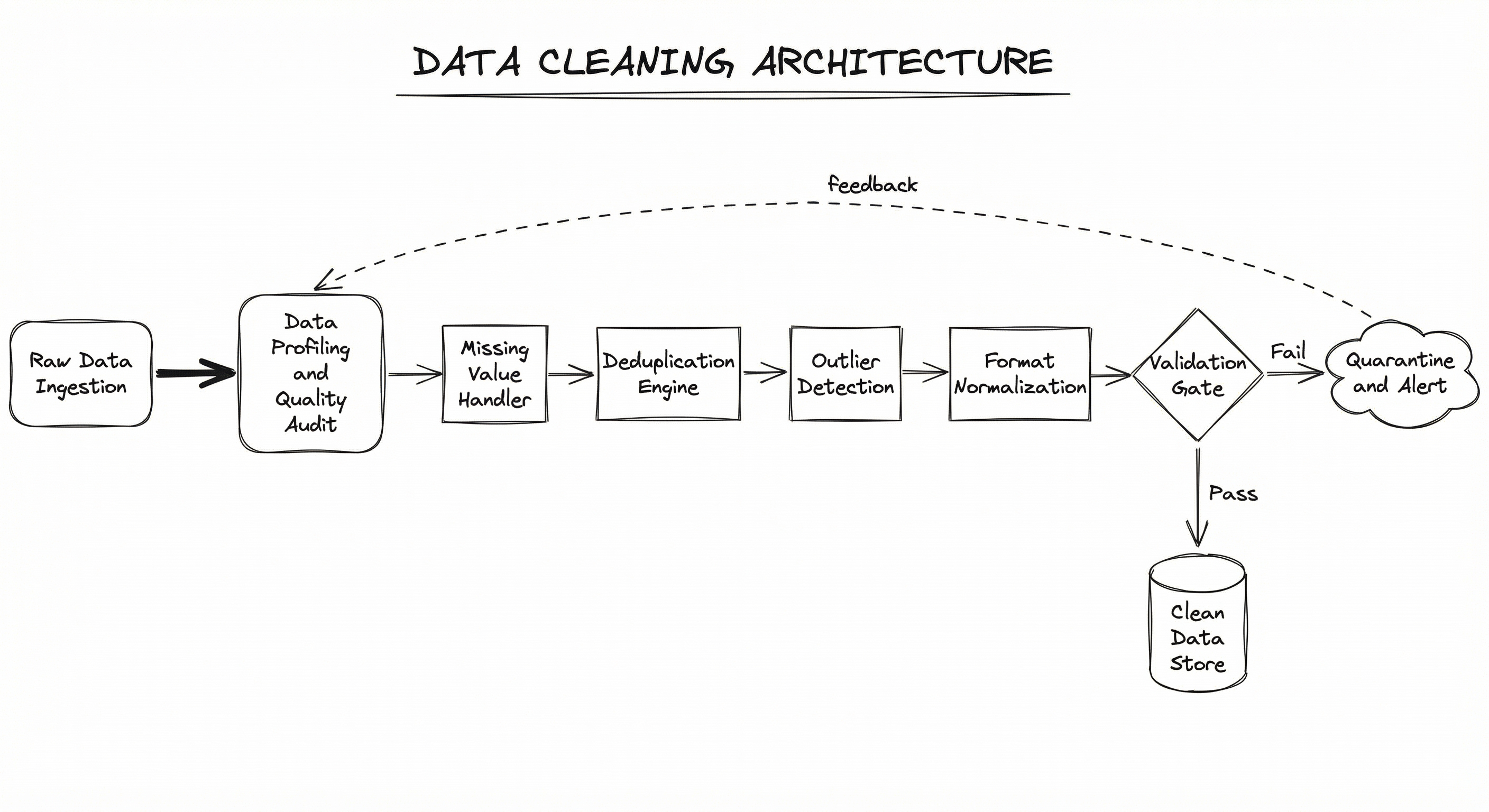
Each stage is independently configurable and observable. The validation gate at the end ensures that only data meeting predefined quality thresholds proceeds to feature engineering. Data that fails validation is quarantined for manual review or re-processing -- never silently dropped.
Key Components
Data Profiler
Generates statistical summaries of the raw dataset: column types, distributions, missing value rates, cardinality, correlation matrices, and data quality scores. Tools like YData Profiling (formerly pandas-profiling) or Great Expectations automate this step. The profiler output drives all downstream cleaning decisions.
Missing Value Handler
Detects and imputes (or drops) missing values according to a configurable strategy per column. Supports multiple methods: mean/median/mode for simple cases, KNN imputation for moderate complexity, MICE (Multiple Imputation by Chained Equations) for statistically rigorous imputation, and model-based imputation (e.g., MissForest using random forests) for complex dependencies.
Deduplication Engine
Identifies and resolves duplicate records. Supports exact matching (hash-based, ), fuzzy matching (edit distance, Jaccard similarity with configurable thresholds), and embedding-based semantic dedup (using vector similarity for near-duplicate text or images). Uses blocking/indexing techniques (MinHash, LSH) to avoid comparisons at scale.
Outlier Detector
Flags anomalous data points using statistical methods (Z-score, IQR), density-based methods (DBSCAN), or tree-based methods (Isolation Forest). Supports configurable actions per column: clip to bounds, replace with median, flag for review, or remove entirely. Domain-specific rules can override statistical detection.
Format Normalizer
Standardizes data formats across the dataset: date parsing to ISO 8601, phone number standardization (E.164), address normalization, Unicode normalization (NFC/NFKD), unit conversion, case folding for text fields, and encoding fixes (UTF-8 enforcement). Critical for Indian datasets where names appear in multiple scripts (Devanagari, Tamil, Telugu, etc.).
Validation Gate
Runs post-cleaning quality checks using tools like Great Expectations or Deequ. Validates that cleaning improved (or at least maintained) data quality metrics. Acts as a circuit breaker: if cleaning degrades quality or introduces unexpected distributions, the pipeline halts and alerts the on-call engineer.
Data Flow
Ingestion: Raw data arrives from upstream sources (databases, APIs, file drops, streaming queues) and is materialized in a staging area (e.g., S3 bucket, staging table).
Profiling: The data profiler scans the staged data and produces a quality report: missing rates per column, duplicate counts, distribution statistics, and schema conformance. This report is stored for auditing and drift detection.
Sequential Cleaning: Data flows through the cleaning stages in order -- missing values first, then deduplication, then outliers, then normalization. This ordering matters: imputing missing values before dedup avoids treating imputed-vs-missing as a difference during matching. Normalizing formats last ensures all upstream transformations work on raw values.
Validation: The cleaned data passes through the validation gate. If all quality assertions pass, data is promoted to the clean data store. If any assertion fails, the batch is quarantined and an alert fires.
Feedback Loop: Quarantined data is reviewed, cleaning rules are updated, and the batch is reprocessed. Over time, the cleaning pipeline learns from its failures and becomes more robust.
A left-to-right flow starting with Raw Data Ingestion, passing through Data Profiling & Quality Audit, Missing Value Handler, Deduplication Engine, Outlier Detection, and Format Normalization, then reaching a Validation Gate that either promotes data to a Clean Data Store or quarantines it with alerts, creating a feedback loop back to profiling.
How to Implement
Two Philosophies of Implementation
There are two broad approaches to implementing data cleaning in ML pipelines:
Approach 1: Scripted pipelines -- Write custom cleaning logic in Pandas, Polars, or PySpark. Maximum flexibility, full control over every transformation, but requires significant engineering effort and testing. This is what most teams start with.
Approach 2: Declarative/framework-based -- Use tools like Great Expectations, Deequ, or Cleanlab that let you declare quality expectations and cleaning rules. Less code, more standardization, but less flexibility for edge cases. This is where mature teams converge.
In practice, most production systems use a hybrid: custom Pandas/Polars scripts for the actual transformations, wrapped in Great Expectations or Deequ for validation and monitoring. Think of it as custom cleaning code with guardrails.
Cost Considerations
For a mid-size Indian startup processing 10M rows daily:
- Pandas on a single EC2 instance (m5.xlarge): ~$50/month (~INR 4,200/month)
- PySpark on EMR (3-node cluster): ~$300/month (~INR 25,200/month)
- Polars on a single instance: Same hardware as Pandas but 5-10x faster, so you can use a smaller instance -- ~$30/month (~INR 2,520/month)
- Managed services (Trifacta/Dataprep): $500-2,000/month (~INR 42,000-1,68,000/month)
The compute cost of cleaning is usually dwarfed by the cost of not cleaning: degraded model performance, customer complaints, and the engineering time spent debugging data issues in production.
import pandas as pd
import numpy as np
from sklearn.impute import KNNImputer
from sklearn.ensemble import IsolationForest

def clean_dataframe(df: pd.DataFrame, config: dict) -> pd.DataFrame:
    """Production-grade data cleaning pipeline.

    Args:
        df: Raw input DataFrame
        config: Cleaning configuration dict
    Returns:
        Cleaned DataFrame with audit log
    """
    audit_log = []
    original_shape = df.shape

    # ---- Step 1: Remove exact duplicates ----
    n_dupes = df.duplicated(subset=config.get('dedup_columns')).sum()
    df = df.drop_duplicates(subset=config.get('dedup_columns'), keep='first')
    audit_log.append(f"Removed {n_dupes} exact duplicates")

    # ---- Step 2: Handle missing values per column ----
    for col, strategy in config.get('missing_strategies', {}).items():
        if col not in df.columns:
            continue
        n_missing = df[col].isna().sum()
        if strategy == 'mean':
            df[col] = df[col].fillna(df[col].mean())
        elif strategy == 'median':
            df[col] = df[col].fillna(df[col].median())
        elif strategy == 'mode':
            df[col] = df[col].fillna(df[col].mode()[0])
        elif strategy == 'drop':
            df = df.dropna(subset=[col])
        elif strategy == 'ffill':
            df[col] = df[col].ffill()
        elif strategy == 'constant':
            fill_val = config.get('fill_values', {}).get(col, 0)
            df[col] = df[col].fillna(fill_val)
        audit_log.append(f"Imputed {n_missing} missing values in '{col}' using {strategy}")

    # ---- Step 3: KNN imputation for remaining numeric NaNs ----
    numeric_cols = df.select_dtypes(include=[np.number]).columns.tolist()
    remaining_nans = df[numeric_cols].isna().sum().sum()
    if remaining_nans > 0:
        imputer = KNNImputer(n_neighbors=5, weights='distance')
        df[numeric_cols] = imputer.fit_transform(df[numeric_cols])
        audit_log.append(f"KNN-imputed {remaining_nans} remaining numeric NaNs")

    # ---- Step 4: Outlier detection with Isolation Forest ----
    outlier_cols = config.get('outlier_columns', numeric_cols)
    if len(outlier_cols) > 0:
        iso = IsolationForest(
            contamination=config.get('contamination', 0.05),
            random_state=42
        )
        outlier_mask = iso.fit_predict(df[outlier_cols]) == -1
        n_outliers = outlier_mask.sum()
        action = config.get('outlier_action', 'flag')
        if action == 'remove':
            df = df[~outlier_mask]
        elif action == 'flag':
            df['is_outlier'] = outlier_mask
        audit_log.append(f"Detected {n_outliers} outliers, action: {action}")

    # ---- Step 5: Text normalization ----
    text_cols = config.get('text_columns', [])
    for col in text_cols:
        if col in df.columns:
            df[col] = (
                df[col]
                .astype(str)
                .str.strip()
                .str.lower()
                .str.replace(r'\s+', ' ', regex=True)
            )

    # ---- Step 6: Type enforcement ----
    for col, dtype in config.get('enforce_types', {}).items():
        if col in df.columns:
            df[col] = pd.to_numeric(df[col], errors='coerce') if dtype == 'numeric' else df[col].astype(dtype)

    print(f"Cleaning complete: {original_shape} -> {df.shape}")
    for entry in audit_log:
        print(f"  - {entry}")

    return df


# --- Usage ---
config = {
    'dedup_columns': ['user_id', 'timestamp'],
    'missing_strategies': {
        'age': 'median',
        'income': 'mean',
        'city': 'mode',
        'notes': 'constant'
    },
    'fill_values': {'notes': 'N/A'},
    'outlier_columns': ['age', 'income', 'transaction_amount'],
    'contamination': 0.03,
    'outlier_action': 'flag',
    'text_columns': ['name', 'address', 'notes'],
    'enforce_types': {'age': 'numeric', 'income': 'numeric'}
}

df_clean = clean_dataframe(df_raw, config)
This pipeline demonstrates a config-driven approach to data cleaning -- each column's cleaning strategy is specified in a dictionary, making the pipeline reusable across datasets. The five-stage flow (dedup -> missing values -> KNN backfill -> outliers -> text normalization) follows the ordering principle described in the architecture section. The audit log tracks every transformation for reproducibility and debugging.
import pandas as pd
import numpy as np
from sklearn.experimental import enable_iterative_imputer  # noqa
from sklearn.impute import IterativeImputer
from sklearn.ensemble import RandomForestRegressor

def mice_impute(df: pd.DataFrame, numeric_cols: list, n_iterations: int = 10) -> pd.DataFrame:
    """Apply MICE imputation using Random Forest as the estimator.

    MICE iteratively models each feature with missing values as a function
    of the other features, cycling through all incomplete features until
    convergence.

    Args:
        df: DataFrame with missing values
        numeric_cols: Columns to impute
        n_iterations: Number of MICE iterations (default 10)
    Returns:
        DataFrame with imputed values
    """
    # Store original missing mask for auditing
    missing_mask = df[numeric_cols].isna()
    missing_rate = missing_mask.mean()
    print("Missing rates before imputation:")
    print(missing_rate[missing_rate > 0].to_string())

    # Configure MICE with MissForest-style estimator
    mice = IterativeImputer(
        estimator=RandomForestRegressor(
            n_estimators=100,
            max_depth=10,
            random_state=42,
            n_jobs=-1
        ),
        max_iter=n_iterations,
        random_state=42,
        verbose=1
    )

    # Fit and transform
    imputed_values = mice.fit_transform(df[numeric_cols])
    df_imputed = df.copy()
    df_imputed[numeric_cols] = imputed_values

    # Audit: compare imputed distributions
    for col in numeric_cols:
        if missing_mask[col].any():
            orig_mean = df[col].mean()
            imputed_mean = df_imputed[col].mean()
            drift = abs(imputed_mean - orig_mean) / (orig_mean + 1e-8)
            print(f"{col}: original mean={orig_mean:.3f}, "
                  f"imputed mean={imputed_mean:.3f}, drift={drift:.2%}")

    return df_imputed


# --- Usage ---
numeric_features = ['age', 'income', 'credit_score', 'tenure_months']
df_clean = mice_impute(df_raw, numeric_features, n_iterations=10)
MICE (Multiple Imputation by Chained Equations) is the gold standard for statistically rigorous missing value imputation. Here we use scikit-learn's IterativeImputer with a Random Forest estimator (this combination is sometimes called MissForest). The key advantage over simple mean/median imputation: MICE preserves inter-feature correlations and produces less biased estimates. The drift check at the end is critical -- if imputation shifts the distribution significantly, it may indicate MNAR data that requires a different approach.
import pandas as pd
import recordlinkage
from recordlinkage.preprocessing import clean as rl_clean

def fuzzy_dedup(df: pd.DataFrame, match_cols: list, threshold: float = 0.85) -> pd.DataFrame:
    """Fuzzy deduplication using record linkage with blocking.

    Uses sorted neighborhood blocking to avoid O(n^2) comparisons,
    then applies string similarity scoring to identify near-duplicates.

    Args:
        df: DataFrame with potential duplicates
        match_cols: Columns to use for matching
        threshold: Similarity threshold (0-1) for considering a match
    Returns:
        Deduplicated DataFrame
    """
    # Preprocess: clean and standardize match columns
    df_clean = df.copy()
    for col in match_cols:
        if df_clean[col].dtype == 'object':
            df_clean[f"{col}_clean"] = rl_clean(df_clean[col])

    clean_cols = [f"{c}_clean" if df_clean[c].dtype == 'object' else c for c in match_cols]

    # Build candidate pairs using sorted neighborhood blocking
    # This reduces O(n^2) to approximately O(n * window_size)
    indexer = recordlinkage.Index()
    indexer.sortedneighbourhood(left_on=clean_cols[0], window=5)
    candidate_pairs = indexer.index(df_clean)
    print(f"Generated {len(candidate_pairs)} candidate pairs from {len(df)} records")

    # Compare candidate pairs
    comparer = recordlinkage.Compare()
    for col in clean_cols:
        if df_clean[col].dtype == 'object' or col.endswith('_clean'):
            comparer.string(col, col, method='jarowinkler', label=col)
        else:
            comparer.numeric(col, col, label=col)

    features = comparer.compute(candidate_pairs, df_clean)

    # Score and threshold
    features['avg_score'] = features.mean(axis=1)
    matches = features[features['avg_score'] >= threshold]
    print(f"Found {len(matches)} duplicate pairs above threshold {threshold}")

    # Resolve: keep first occurrence, mark rest for removal
    to_remove = set()
    for idx_a, idx_b in matches.index:
        if idx_a not in to_remove:
            to_remove.add(idx_b)

    df_deduped = df.drop(index=list(to_remove))
    print(f"Removed {len(to_remove)} fuzzy duplicates: {len(df)} -> {len(df_deduped)}")

    return df_deduped


# --- Usage: Dedup an Indian e-commerce product catalog ---
df_products = pd.DataFrame({
    'product_name': ['Samsung Galaxy S24 Ultra', 'samsung galaxy s24ultra',
                     'iPhone 15 Pro Max', 'Apple iPhone 15 ProMax 256GB'],
    'brand': ['Samsung', 'samsung', 'Apple', 'Apple'],
    'price': [1_29_999, 1_29_999, 1_59_900, 1_59_900]
})

df_clean = fuzzy_dedup(df_products, match_cols=['product_name', 'brand'], threshold=0.80)
This example tackles a problem every Indian e-commerce platform faces: the same product listed with slightly different names, capitalization, and formatting. The record linkage library uses sorted neighborhood blocking to avoid the pairwise comparison problem, then applies Jaro-Winkler string similarity to score candidate pairs. The threshold of 0.80-0.85 works well for product names; lower thresholds catch more duplicates but increase false positives.
import great_expectations as gx

def validate_cleaned_data(df, suite_name="post_cleaning_suite"):
    """Validate cleaned data using Great Expectations.

    Defines expectations for data quality after cleaning
    and returns a validation report.
    """
    context = gx.get_context()

    # Create a data source from our DataFrame
    data_source = context.data_sources.add_pandas(name="cleaned_data")
    data_asset = data_source.add_dataframe_asset(name="df")
    batch_definition = data_asset.add_batch_definition_whole_dataframe("batch")
    batch = batch_definition.get_batch(batch_parameters={"dataframe": df})

    # Create expectation suite
    suite = context.suites.add(
        gx.ExpectationSuite(name=suite_name)
    )

    # ---- Define expectations ----
    # No nulls in critical columns
    suite.add_expectation(
        gx.expectations.ExpectColumnValuesToNotBeNull(column="user_id")
    )
    suite.add_expectation(
        gx.expectations.ExpectColumnValuesToNotBeNull(column="timestamp")
    )

    # Value ranges
    suite.add_expectation(
        gx.expectations.ExpectColumnValuesToBeBetween(
            column="age", min_value=0, max_value=120
        )
    )
    suite.add_expectation(
        gx.expectations.ExpectColumnValuesToBeBetween(
            column="transaction_amount", min_value=0, max_value=10_00_000  # INR 10 lakh
        )
    )

    # Uniqueness
    suite.add_expectation(
        gx.expectations.ExpectColumnValuesToBeUnique(column="user_id")
    )

    # Column completeness threshold
    suite.add_expectation(
        gx.expectations.ExpectColumnValuesToNotBeNull(
            column="email", mostly=0.95  # Allow 5% nulls
        )
    )

    # Run validation
    validation_definition = context.validation_definitions.add(
        gx.ValidationDefinition(
            name="post_clean_validation",
            data=batch_definition,
            suite=suite
        )
    )
    result = validation_definition.run(batch_parameters={"dataframe": df})

    if result.success:
        print("All quality checks PASSED")
    else:
        print("Quality checks FAILED:")
        for r in result.results:
            if not r.success:
                print(f"  FAIL: {r.expectation_config.type} "
                      f"on '{r.expectation_config.kwargs.get('column', 'N/A')}'")

    return result


# --- Usage ---
result = validate_cleaned_data(df_clean)
Great Expectations is the industry standard for data validation in ML pipelines. This example defines a suite of post-cleaning quality checks: no nulls in critical columns, value range constraints (note the INR-denominated transaction amount cap), uniqueness checks for IDs, and a mostly parameter that allows controlled levels of incompleteness. If any expectation fails, the pipeline halts rather than passing dirty data downstream.
# data_cleaning_config.yaml
# Configuration for the data cleaning pipeline

pipeline:
  name: user_transactions_cleaning
  version: "2.1.0"
  schedule: "0 */4 * * *"  # Every 4 hours

profiling:
  tool: ydata-profiling
  output_path: s3://data-quality/profiles/
  alert_on:
    missing_rate_threshold: 0.30
    duplicate_rate_threshold: 0.05

missing_values:
  default_strategy: median
  per_column:
    user_id: drop          # Cannot impute identifiers
    age: knn               # Correlated with other demographics
    income: mice            # Complex dependencies
    city: mode              # Categorical
    email: constant         # Fill with '[email protected]'
    transaction_amount: median
  knn_params:
    n_neighbors: 5
    weights: distance
  mice_params:
    max_iter: 10
    estimator: random_forest

deduplication:
  exact:
    columns: [user_id, timestamp]
    keep: first
  fuzzy:
    enabled: true
    columns: [name, email, phone]
    method: jaro_winkler
    threshold: 0.88
    blocking_key: city     # Only compare within same city

outliers:
  method: isolation_forest
  contamination: 0.03
  columns: [age, income, transaction_amount]
  action: flag             # flag | clip | remove
  clip_bounds:
    age: [0, 120]
    income: [0, 50000000]  # INR 5 crore
    transaction_amount: [0, 1000000]  # INR 10 lakh

normalization:
  text_columns:
    - name: [strip, lower, unicode_nfc]
    - address: [strip, lower, normalize_whitespace]
    - city: [strip, title_case]
  date_columns:
    - timestamp: ISO8601
    - created_at: ISO8601
  phone_columns:
    - phone: E164_IN       # Indian phone format

validation:
  tool: great_expectations
  suite: post_cleaning_v2
  fail_action: quarantine  # quarantine | warn | block
  expectations:
    - column: user_id
      type: not_null
    - column: age
      type: between
      min: 0
      max: 120
    - column: email
      type: not_null
      mostly: 0.95
Common Implementation Mistakes
- ●
Imputing before splitting: Fitting an imputer on the full dataset (including test data) causes data leakage. Always fit imputation statistics on the training set only, then transform both train and test. This is the #1 mistake in Kaggle kernels and it silently inflates your validation metrics.
- ●
Using mean imputation blindly: Mean imputation reduces variance and weakens correlations between features. For any dataset with more than 5% missing values, use KNN or MICE instead. Mean imputation literally shrinks your feature space toward the center -- destroying the very patterns your model needs to learn.
- ●
Dropping columns with any missing values: A column with 30% missing data still contains 70% useful information. Only drop a column if its missing rate exceeds 60-70% AND you cannot determine a reasonable imputation strategy. Even then, consider whether the missingness pattern itself is informative.
- ●
Ignoring the missing data mechanism: Applying MCAR-appropriate methods (like listwise deletion) to MNAR data introduces systematic bias. Always test for missingness patterns using Little's MCAR test or by examining correlations between the missingness indicator and other features.
- ●
Deduplicating without a merge strategy: When two duplicate records have conflicting values (e.g., different phone numbers), simply keeping the first occurrence loses information. Define an explicit merge strategy: take the most recent, the most complete, or the mode across duplicates.
- ●
Not versioning cleaning transformations: If you cannot reproduce exactly what cleaning was applied to a training dataset, you cannot debug model regressions. Log every transformation with timestamps, parameters, and row counts. Treat your cleaning pipeline with the same rigor as your model code.
When Should You Use This?
Use When
Your dataset has more than 1% missing values -- even small amounts of missingness can bias model estimates if not handled properly
You are merging data from multiple sources with different schemas, naming conventions, or quality standards (common in Indian enterprises integrating legacy systems)
Your ML model's performance has plateaued and you suspect data quality issues rather than model capacity limitations
You are building a production pipeline where data arrives continuously and quality can degrade without automated checks
Your dataset contains user-generated content (product reviews, addresses, names) with inconsistent formatting and potential duplicates
Regulatory or compliance requirements demand auditable data transformations (financial services, healthcare, DPDP Act in India)
You are preparing training data for a model that will make high-stakes decisions (credit scoring, medical diagnosis, fraud detection)
Avoid When
Your dataset is already clean and validated from a trusted upstream source with its own quality guarantees -- re-cleaning adds latency without benefit
You are working with small, manually curated datasets (<100 rows) where visual inspection is faster and more reliable than automated pipelines
The data is intentionally sparse (e.g., one-hot encoded features, sparse user-item interaction matrices) -- 'missing' values are semantically zero, not unknown
Your model is inherently robust to noise (e.g., gradient-boosted trees with built-in missing value handling via XGBoost or LightGBM's native NaN support)
Aggressive cleaning would remove the very signals you need -- for example, outlier detection in a fraud model would remove the fraud cases themselves
You are in a rapid prototyping phase where the cost of building a cleaning pipeline exceeds the expected improvement in model quality
Key Tradeoffs
The Central Tension: Cleaning Too Little vs. Too Much
Under-cleaning leaves noise that your model will memorize. Over-cleaning removes genuine signal -- rare but real data points that represent the edge cases your model needs to learn. The optimal cleaning level depends on your task, your model, and your tolerance for different types of errors.
| Cleaning Dimension | Conservative (Less Cleaning) | Aggressive (More Cleaning) |
|---|---|---|
| Missing values | Keep rows, impute with simple stats | Drop rows with >20% missing features |
| Outliers | Flag only, let model decide | Remove all points beyond 2.5 sigma |
| Duplicates | Exact match only | Fuzzy match with 0.75 threshold |
| Text normalization | Case-fold and strip whitespace | Full lemmatization + stopword removal |
| Risk | Model learns noise | Model loses rare but real patterns |
Compute-Quality Tradeoff
Simple methods (mean imputation, exact dedup) are fast -- -- but produce lower-quality results. Advanced methods (MICE, fuzzy dedup with embedding similarity) produce higher-quality results but cost significantly more compute. For a 100M-row dataset:
- Mean imputation: ~30 seconds on a single machine
- KNN imputation (): ~15 minutes (pairwise distance computation)
- MICE (10 iterations): ~2 hours (iterative model fitting)
At Indian cloud pricing (~INR 7/hour for a c5.2xlarge), that is the difference between INR 0.06 and INR 14 per cleaning run. For daily pipelines, this adds up.
Rule of Thumb: Start with simple methods. Monitor model performance. Upgrade cleaning complexity only for columns where the downstream model is most sensitive. Use feature importance scores to prioritize cleaning investment.
Alternatives & Comparisons
Data validation checks whether data conforms to expectations (schema, ranges, constraints) but does not fix issues. Data cleaning detects and repairs problems. In practice, you need both: validation as the quality gate, cleaning as the repair mechanism. Use validation alone when you have control over the upstream source and can reject bad data at ingestion.
Data transformation creates new representations of data (log transforms, polynomial features, embeddings). Data cleaning fixes errors in existing data. The line blurs when normalization is involved: standardizing a column to zero-mean unit-variance is both cleaning (fixing scale inconsistencies) and transformation (creating a model-ready feature). Cleaning always precedes transformation in the pipeline.
Deduplication is a specialized sub-problem within data cleaning focused exclusively on identifying and merging duplicate records. When dedup is your primary concern (e.g., entity resolution across databases, catalog deduplication for e-commerce), a dedicated dedup system with blocking, matching, and merge logic outperforms a general-purpose cleaning pipeline. For everything else, dedup is one stage within the broader cleaning flow.
Normalization standardizes data formats and scales without altering semantics -- unit conversion, date parsing, Unicode normalization, min-max scaling. It is a subset of data cleaning focused purely on consistency. When your data is complete and accurate but just inconsistently formatted (common after merging data from Indian state-level systems with different conventions), normalization alone may suffice.
Pros, Cons & Tradeoffs
Advantages
Directly improves model performance: Studies consistently show that cleaning training data yields 2-10% accuracy gains, often exceeding the gains from model architecture changes. For a credit scoring model at a company like Cred or BharatPe, that improvement translates to crores in reduced defaults.
Reduces training time and cost: Clean data converges faster. Models trained on noisy data require more epochs to learn through the noise, wasting GPU hours. At INR 150-300/hour for cloud GPUs, this matters.
Enables reliable feature engineering: Features computed from dirty data propagate errors downstream. A
customer_lifetime_valuefeature computed from duplicate transaction records will be systematically inflated, biasing every model that uses it.Catches data pipeline bugs early: A cleaning pipeline with validation gates acts as a canary for upstream data issues -- schema changes, API failures, ETL bugs. It is cheaper to catch these at cleaning time than after a model is deployed.
Improves model fairness and reduces bias: Missing data and duplicates are often non-random across demographic groups. Systematic cleaning reduces the risk of models that perform well on the majority but fail on underrepresented groups -- a critical concern under India's emerging AI governance framework.
Makes models interpretable: When stakeholders ask 'why did the model predict X?', clean data makes the explanation coherent. Dirty data produces explanations that reference artifacts rather than real patterns.
Disadvantages
Consumes significant engineering time: Building and maintaining a production cleaning pipeline is not a one-time cost. Data distributions shift, new data sources introduce new quality issues, and cleaning rules need constant updating.
Risk of information loss: Overly aggressive cleaning (dropping rows, clipping outliers, aggressive dedup) can remove genuine rare events that are critical for certain tasks. Fraud detection, rare disease prediction, and anomaly detection are especially vulnerable.
Imputation introduces artificial patterns: Any imputation method makes assumptions about the data-generating process. If those assumptions are wrong (e.g., assuming MAR when data is MNAR), imputed values can introduce systematic biases that are harder to detect than the original missing values.
Computational cost at scale: MICE imputation on a 100M-row dataset with 50 features can take hours on a large cluster. Fuzzy deduplication with embedding similarity is even more expensive. For real-time pipelines, the cleaning latency may exceed the acceptable window.
Domain expertise bottleneck: Many cleaning decisions require domain knowledge -- is 150 a valid age for a tree species dataset? Is a transaction of INR 50 lakh suspicious or normal for a B2B platform? Automating these decisions is hard, and wrong automation is worse than no automation.
Reproducibility challenges: If cleaning logic changes between model training and inference, or between training runs, you get training-serving skew. Versioning cleaning pipelines and ensuring consistent application is non-trivial.
Failure Modes & Debugging
Data leakage through imputation
Cause
Fitting an imputer (e.g., KNNImputer, MICE) on the entire dataset including test/validation data before splitting. The imputed values in the test set now contain information from the test set's own statistics.
Symptoms
Validation metrics are significantly higher than production performance. The model appears to generalize well during development but degrades once deployed. A/B test results consistently underperform offline evaluations.
Mitigation
Always split data before any imputation. Fit imputers on the training set only, then transform() (not fit_transform()) on validation and test sets. Use scikit-learn Pipeline to encapsulate the imputer and model together, ensuring correct sequencing during cross-validation.
Survivor bias from aggressive row dropping
Cause
Dropping all rows with any missing values (df.dropna()) when missingness is correlated with the target variable (MNAR). The remaining 'clean' data is no longer representative of the true population.
Symptoms
Model performs well on the cleaned training data but poorly on production data where missing values are common. Performance degrades specifically for the subpopulation most likely to have missing data (e.g., low-income users who skip optional fields, rural users with spotty connectivity).
Mitigation
Always analyze the missingness mechanism before choosing a strategy. Use Little's MCAR test or compare distributions of observed vs. missing subgroups. For MNAR data, consider pattern-mixture models or selection models rather than simple imputation. At minimum, create a binary is_missing indicator feature that lets the model learn from the missingness pattern.
False-positive deduplication
Cause
Fuzzy matching threshold set too low, causing genuinely distinct records to be merged. Common with common Indian names (e.g., 'Rahul Sharma' in Delhi vs. 'Rahul Sharma' in Mumbai being merged as duplicates).
Symptoms
Record count drops more than expected after dedup. Users complain that their accounts or orders have been merged with someone else's. Model predictions for affected users become incoherent because features from multiple real entities are combined.
Mitigation
Always combine name similarity with additional discriminating features (phone, email, address, PIN code). Set conservative thresholds (0.90+) and manually review matches in the 0.80-0.90 band. Implement a human-in-the-loop review for ambiguous matches, especially for high-stakes domains like financial services.
Distribution shift from over-cleaning
Cause
Outlier removal eliminates genuine extreme values, or aggressive normalization destroys distributional properties. The cleaned data no longer represents the real-world distribution the model will encounter.
Symptoms
Model underperforms on tail events (high-value transactions, extreme weather conditions, surge pricing scenarios). The gap between training and production distributions widens over time as more edge cases are encountered.
Mitigation
Before removing outliers, check if they correspond to real phenomena. Use domain experts to validate outlier boundaries. Consider winsorization (clipping to percentile bounds like 1st-99th) instead of removal -- this preserves the extreme-value signal while limiting its magnitude. Always compare training data distributions with a held-out production sample.
Silent schema drift in continuous pipelines
Cause
Upstream data source changes a column type (e.g., price from integer to string with currency symbol), adds new columns, or changes encoding. The cleaning pipeline does not detect the change and either fails silently or produces corrupted output.
Symptoms
Sudden spike in cleaning pipeline failures, or worse, no failures but a spike in downstream model errors. New categories appear in categorical columns that the imputer does not know how to handle. Numeric columns suddenly contain NaN where they previously did not.
Mitigation
Implement schema validation at the ingestion stage using tools like Great Expectations or Deequ. Define expectations for column types, value ranges, and allowed categories. Alert immediately when schema drift is detected. Version your data schemas alongside your code.
Imputation-induced multicollinearity
Cause
Using a single imputation method (e.g., regression imputation) that creates deterministic relationships between features. The imputed values artificially inflate correlations, leading to multicollinearity in downstream linear models.
Symptoms
Linear regression coefficients become unstable (high variance, sign flips). Feature importance scores are unreliable. Model confidence intervals are artificially narrow.
Mitigation
Use multiple imputation (creating several imputed datasets and pooling results) to properly account for imputation uncertainty. Alternatively, use tree-based models (XGBoost, LightGBM) that are robust to multicollinearity. Monitor the correlation matrix before and after imputation and flag any correlation that increases by more than 0.15.
Placement in an ML System
Where Does Data Cleaning Sit?
Data cleaning is the first major transformation step after raw data enters the ML pipeline. It sits between data ingestion (which handles transport and storage) and feature engineering (which creates model-ready representations).
In practice, the boundary between cleaning and ingestion is fuzzy. Many ingestion systems perform basic quality checks (schema validation, type casting) as data arrives. But the heavy lifting -- imputation, dedup, outlier handling -- happens in a dedicated cleaning stage.
Data cleaning also has a feedback relationship with data validation. Validation detects problems; cleaning fixes them. In mature systems like those at Amazon (using Deequ) or Airbnb (using their Midas framework), cleaning and validation form a tight loop: validate -> clean -> re-validate -> either promote to the clean store or quarantine for review.
Critical Insight: Data cleaning is not a one-time operation. In production ML systems, it runs continuously -- every new batch of data passes through the cleaning pipeline. The cleaning rules themselves evolve as data distributions shift and new edge cases emerge. Treat your cleaning pipeline as a living system, not a static script.
Pipeline Stage
Data Processing / Preprocessing
Upstream
- data-ingestion
- data-validation
Downstream
- feature-extraction
- data-transformation
- normalization
- model-training
Scaling Bottlenecks
The primary bottlenecks are memory (loading entire datasets for global imputation), compute (iterative methods like MICE scale poorly beyond 10M rows), and I/O (reading and writing large datasets during multi-stage cleaning).
Specific numbers:
- KNN imputation on rows with features: for naive implementation. With approximate nearest neighbors, .
- Fuzzy deduplication on records: for brute-force, with MinHash/LSH blocking.
- MICE with iterations on features: where is the cost of fitting one imputation model.
For datasets exceeding 100M rows, consider:
- Chunked processing with Polars or Dask (avoid loading full dataset into memory)
- Approximate methods: random sampling for imputer fitting, MinHash for dedup
- Distributed execution: PySpark with Deequ for cleaning at warehouse scale
- Incremental cleaning: only clean new/changed records, not the full dataset
Production Case Studies
Airbnb built Midas, an internal data quality framework that establishes a 'gold standard' for certified data models. Midas serves as a shared foundation across business reporting, product analytics, experimentation, and ML/AI. The system enforces data quality contracts: producers certify that their data meets defined quality thresholds before consumers (including ML pipelines) can use it.
Midas became the single source of truth for data quality at Airbnb, reducing data-related incidents and enabling teams to spend more time on modeling rather than debugging data issues. Certified datasets serve all analytics and ML workloads company-wide.
Amazon developed Deequ, an open-source library built on Apache Spark for defining 'unit tests for data.' Deequ computes data quality metrics (completeness, uniqueness, distribution statistics) and verifies constraints on large datasets. It is used internally at Amazon for verifying the quality of many large production datasets and powers Amazon SageMaker Model Monitor for continuous data quality monitoring.
Deequ processes millions of data quality checks across Amazon's production datasets daily. The library automatically detects anomalies in data distributions and alerts teams before degraded data reaches ML models, preventing model performance regressions at scale.
Flipkart's product catalog contains millions of SKUs from thousands of sellers, resulting in massive data quality challenges: duplicate listings (the same phone listed with different names), inconsistent specifications (RAM listed as '8GB', '8 GB', '8gb'), and missing attributes. Their engineering team built automated cleaning pipelines that combine fuzzy matching for deduplication, NLP-based attribute extraction, and image similarity for visual dedup to maintain catalog quality.
Reduced duplicate product listings by approximately 30% in high-volume categories, improving catalog quality, reducing customer confusion, and decreasing return rates on misidentified products.
DoorDash uses LLMs combined with OCR and multimodal models to automatically transcribe and standardize restaurant menu photos at scale, implementing ML guardrails and data cleaning pipelines to canonicalize capitalization, synonyms, and tokenization.
Automated menu transcription replaced costly manual data entry, with multimodal LLMs proving excellent at understanding menu layouts and visual cues that traditional OCR systems struggled with.
Netflix's data engineering team built a scalable data lifecycle management system to handle the 'data deluge' -- petabytes of viewing data, A/B test logs, and content metadata. Their Media Infrastructure team uses a Garbage Collector (GC) architecture that monitors and cleans up file objects using Kafka queues and horizontally scalable GC workers. Data validation and cleaning are embedded throughout their pipeline to ensure ML models for recommendation, content optimization, and search receive high-quality inputs.
The system manages Netflix's multi-petabyte data lake, ensuring data freshness and quality for ML models serving 200M+ subscribers globally while reducing storage costs through automated lifecycle management.
Tooling & Ecosystem
The foundational Python library for data manipulation and cleaning. Provides dropna(), fillna(), duplicated(), drop_duplicates(), string methods, and type conversion. Best for datasets that fit in memory (<10GB). Pandas 2.x introduced Apache Arrow backends for improved performance.
A blazingly fast DataFrame library written in Rust with Python bindings. Offers 5-10x performance over Pandas for typical data cleaning operations through multi-threaded execution and query optimization. Handles datasets larger than RAM via streaming. Increasingly the default choice for performance-sensitive cleaning pipelines.
The industry-standard open-source framework for data validation and quality testing. Lets you define declarative 'expectations' (e.g., 'this column should have no nulls', 'values should be between 0 and 100') and automatically validates data against them. Integrates with Airflow, Spark, and most data orchestrators.
Amazon's open-source library for data quality validation at scale, built on Apache Spark. Defines 'unit tests for data' -- computes metrics like completeness, uniqueness, and distribution statistics. Powers Amazon SageMaker Model Monitor. PyDeequ provides Python bindings.
Automatically detects label errors in ML datasets using confident learning algorithms. Identifies mislabeled data points that traditional cleaning methods miss. Found label errors in MNIST, ImageNet, and Amazon Reviews. Essential for data-centric AI workflows where label quality matters as much as feature quality.
Generates comprehensive data quality reports with one line of code: missing value analysis, duplicate detection, distribution plots, correlation matrices, and data type warnings. Supports both Pandas and Spark DataFrames. The starting point for any data cleaning effort -- profile before you clean.
Provides SimpleImputer (mean, median, mode, constant), KNNImputer (KNN-based), and IterativeImputer (MICE-style) with scikit-learn Pipeline integration. The IterativeImputer is experimental but widely used for production MICE workflows. Ensures imputation is properly chained with model training to prevent data leakage.
A Python library for record linkage and fuzzy deduplication. Provides blocking, comparison (string similarity, numeric, geographic), classification, and evaluation tools. Supports sorted neighborhood and Q-gram indexing to avoid comparisons. Used for entity resolution across datasets.
Research & References
Northcutt, Jiang & Chuang (2021)Journal of Artificial Intelligence Research (JAIR)
Introduced the confident learning framework for identifying label errors in datasets by estimating the joint distribution between noisy and true labels. Found pervasive label errors in major benchmarks including MNIST and ImageNet. Powers the open-source Cleanlab library.
Rekatsinas, Chu, Ilyas & Re (2017)Proceedings of the VLDB Endowment
Proposed a probabilistic framework for data cleaning that unifies integrity constraints, external knowledge, and statistical properties. Achieved ~90% precision and ~76% recall on diverse datasets, yielding 2x F1 improvement over prior methods.
Zha, Bhat, Lai, Yang, Jiang, Zhong & Hu (2023)arXiv preprint
Comprehensive survey of the data-centric AI paradigm covering data collection, labeling, preparation (cleaning), and quality evaluation. Provides a taxonomy of data cleaning approaches and their relationship to downstream model performance.
Li, Song, Hou, Yu & Chen (2024)Data Science and Engineering (Springer)
Reviews three essential tasks for cleaning relational data -- error detection, data repairing, and data imputation -- using both traditional and AI-based techniques. Covers the evolution from rule-based to ML-driven cleaning approaches.
Azur, Stuart, Frangakis & Leaf (2011)International Journal of Methods in Psychiatric Research
Foundational tutorial on MICE methodology. Explains the chained equations approach for handling missing data with varying types (continuous, binary, categorical) and provides practical guidelines for implementation and convergence diagnostics.
Schelter, Lange, Schmidt, Celikel, Biessmann & Grafberger (2018)Proceedings of the VLDB Endowment
Describes Amazon's Deequ system for defining 'unit tests for data' at scale. Introduces the concept of constraint suggestion and verification for large datasets, and reports on deployment experience at Amazon where Deequ validates billions of records daily.
Interview & Evaluation Perspective
Common Interview Questions
- ●
You have a dataset with 25% missing values in a critical feature. Walk me through your approach to handling this.
- ●
How would you design a data cleaning pipeline for an e-commerce platform processing 50M product listings with duplicates across multiple sellers?
- ●
Explain the difference between MCAR, MAR, and MNAR. Why does it matter for your imputation strategy?
- ●
Your model's accuracy dropped 3% after a data pipeline change. How would you debug this?
- ●
When should you impute missing values vs. drop rows vs. create a missing indicator feature?
- ●
How do you prevent data leakage when imputing missing values in a cross-validation setup?
- ●
Design a deduplication system for an Aadhaar-like identity database with 1 billion records.
Key Points to Mention
- ●
Always analyze the missing data mechanism (MCAR/MAR/MNAR) before choosing an imputation strategy. This is the foundational decision that everything else follows from.
- ●
MICE and MissForest are the gold standards for multivariate imputation because they preserve inter-feature correlations, unlike mean/median imputation which shrinks variance.
- ●
Data leakage through imputation is one of the most common and hardest-to-detect bugs in ML pipelines. Always fit imputers on training data only.
- ●
For deduplication at scale, blocking (reducing the comparison space from to ) is not optional -- it is essential. Discuss MinHash, LSH, or sorted neighborhood indexing.
- ●
Data cleaning should be config-driven and auditable: every transformation should be logged with parameters, timestamps, and row counts. This is not just good practice -- it is often a regulatory requirement.
- ●
The data-centric AI insight: for many real-world problems, improving data quality yields larger gains than improving model architecture. Quantify this with examples from your experience.
Pitfalls to Avoid
- ●
Saying 'I would just drop the NaN rows' without considering the missingness mechanism or the impact on the remaining data distribution.
- ●
Ignoring the computational cost of advanced imputation methods at scale. MICE on 100M rows is not the same as MICE on a Kaggle dataset -- always discuss scalability.
- ●
Treating data cleaning as a one-time preprocessing step rather than a continuous pipeline operation with monitoring, alerting, and feedback loops.
- ●
Forgetting that outlier removal in a fraud detection or anomaly detection context would remove the very signal you are trying to model.
Senior-Level Expectation
A senior candidate should discuss the end-to-end lifecycle: data profiling to understand quality characteristics, selecting imputation strategies based on missingness mechanisms (with statistical tests like Little's MCAR test), implementing cleaning as a reproducible pipeline (not a notebook), validating cleaning quality with tools like Great Expectations, monitoring for data drift post-deployment, and handling the feedback loop when production data reveals new cleaning needs. They should be able to reason about the cost-quality tradeoff -- when is mean imputation 'good enough' vs. when do you need MICE -- and back this reasoning with computational cost estimates. They should also discuss how cleaning decisions affect model fairness: if missingness is correlated with protected attributes (common in Indian datasets where rural populations have more missing data), naive cleaning can amplify existing biases.
Summary
What We Covered
Data cleaning is the systematic process of detecting and correcting corrupt, incomplete, duplicate, and inconsistent records in datasets destined for ML model training and inference. It is not a preliminary chore -- it is a core engineering discipline that directly determines model quality, fairness, and reliability.
The key concepts and decisions:
-
Missing value handling requires understanding the missingness mechanism (MCAR, MAR, MNAR) before choosing a strategy. Simple methods (mean, median) work for low missing rates with independent features. MICE and KNN imputation preserve inter-feature correlations and produce statistically valid estimates for moderate-to-high missing rates. Always fit imputers on training data only to prevent data leakage.
-
Deduplication spans from exact matching (, hash-based) to fuzzy matching (edit distance, Jaccard similarity) to embedding-based semantic dedup. At scale, blocking techniques (MinHash, LSH, sorted neighborhood) are essential to avoid comparisons. False positives in dedup can be as damaging as missed duplicates -- always define a merge strategy for conflicting values.
-
Outlier detection methods range from statistical (Z-score, IQR) to model-based (Isolation Forest, DBSCAN). The critical decision is whether an outlier is a data error (remove it) or a genuine rare event (keep it). Winsorization offers a middle ground. In production, combine automated detection with domain-specific rules.
-
Production pipelines should be config-driven, auditable, and validated. Tools like Great Expectations and Deequ provide the validation gates. Pandas and Polars handle the transformations. The pipeline should run continuously with monitoring and alerting -- not as a one-time notebook.
Data cleaning is where the data-centric AI philosophy meets engineering reality. The teams that invest in robust, automated, well-monitored cleaning pipelines consistently outperform teams that treat cleaning as an afterthought -- regardless of how sophisticated their models are. As Andrew Ng observed, for most real-world ML problems, better data beats a better model.