Time-Series DB in Machine Learning
Every ML system in production generates a relentless stream of timestamped data: training loss curves, inference latencies, prediction confidence scores, feature drift statistics, GPU utilization, and throughput counters. Storing and querying this data efficiently is not optional -- it is the foundation of observability for machine learning.
A time-series database (TSDB) is a storage engine purpose-built for ingesting, compressing, and querying data points that are naturally ordered by time. Unlike general-purpose relational databases, TSDBs exploit the temporal structure of the data to achieve compression ratios of 10-70x and query speeds that make real-time dashboards and alerting practical.
Why does this matter for ML specifically? Because model degradation is a time-dependent phenomenon. A recommendation model that was accurate last Tuesday may be drifting today. Detecting that drift requires comparing metrics across time windows -- exactly the operation TSDBs are optimized for. From Zerodha monitoring trade execution latency with Prometheus and VictoriaMetrics, to Netflix ingesting billions of metrics per minute into Atlas, time-series databases are the silent backbone of every serious ML monitoring stack.
In this guide, we will cover the internal architecture of TSDBs, the key algorithms (delta-of-delta compression, LSM trees, continuous aggregates), practical implementation with InfluxDB, TimescaleDB, and Prometheus, and the decision framework for choosing the right TSDB for your ML workload.
Concept Snapshot
- What It Is
- A database engine optimized for ingesting, storing, compressing, and querying timestamped data points at high throughput with time-range-oriented retrieval patterns.
- Category
- Storage
- Complexity
- Intermediate
- Inputs / Outputs
- Inputs: timestamped metric data points (timestamp, metric name, value, tags/labels). Outputs: time-range query results, aggregated rollups, alerting triggers, continuous aggregate views.
- System Placement
- Sits downstream of metrics collectors, model serving endpoints, and training jobs; upstream of dashboards (Grafana), alerting systems, and drift detection pipelines.
- Also Known As
- TSDB, time-series store, metrics database, temporal database, telemetry store
- Typical Users
- ML Engineers, MLOps Engineers, SRE / Platform Engineers, Data Engineers, Infrastructure Engineers
- Prerequisites
- Basic database concepts (indexing, queries), Understanding of metrics and monitoring, Familiarity with time-series data (timestamps, intervals), Basic knowledge of compression algorithms
- Key Terms
- retention policydownsamplingcontinuous aggregatescardinalitywrite-ahead logdelta-of-delta compressionPromQLFluxhypertablecompaction
Why This Concept Exists
The Problem: ML Systems Generate Enormous Volumes of Timestamped Data
Consider a moderately complex ML system serving 1,000 requests per second. For each request, you want to track: inference latency (p50, p95, p99), prediction confidence, input feature distributions (say, 50 features), model version, GPU memory usage, and batch queue depth. That is roughly 60 distinct metrics per request, producing 60,000 data points per second -- or 5.2 billion data points per day.
A traditional relational database like PostgreSQL can handle maybe 10,000-50,000 inserts per second on a well-tuned instance. You would need a cluster of 10+ PostgreSQL nodes just to keep up with the write load, and queries over time ranges would be painfully slow because B-tree indices are not optimized for temporal range scans.
Why General-Purpose Databases Fall Short
The mismatch is fundamental. Relational databases are designed for random-access read/write patterns with ACID guarantees. Time-series workloads are almost the opposite:
- Writes are append-only: new data always arrives at the current timestamp. You almost never update historical data points.
- Reads are sequential and range-based: "give me all latency values between 2:00 PM and 2:15 PM" is the dominant query pattern.
- Data has natural temporal locality: recent data is queried far more often than old data.
- Individual data points have low value; aggregates have high value: nobody cares about a single latency measurement, but the P99 over the last hour is critical.
These characteristics enable specialized optimizations -- columnar storage, delta-of-delta timestamp compression, automatic downsampling -- that general databases cannot exploit.
The Evolution: From RRDtool to Modern TSDBs
The lineage goes back to RRDtool (1999), which introduced round-robin databases with fixed retention. Then came Graphite (2006), which popularized the whisper file format and hierarchical metric naming. The modern era began with OpenTSDB (2010, built on HBase), followed by InfluxDB (2013), Prometheus (2012, open-sourced 2015), and TimescaleDB (2017).
Each generation improved on compression, query expressiveness, and operational simplicity. Today's TSDBs like QuestDB can ingest 4-11 million rows per second on a single node, while VictoriaMetrics achieves 10x lower memory usage than InfluxDB for the same dataset.
Key Takeaway: Time-series databases exist because the append-heavy, range-scan-dominant, high-cardinality nature of ML metrics data is fundamentally mismatched with the random-access, B-tree-indexed architecture of general-purpose databases. TSDBs exploit temporal structure to deliver 10-100x better write throughput, compression, and query performance for this specific workload.
Core Intuition & Mental Model
The Library Analogy
Imagine a library where new books arrive every second and are always shelved at the end of the shelf -- you never insert a book in the middle. Readers almost always ask for "all books that arrived in the last hour" or "the average page count of books from last Tuesday." Would you organize this library with a traditional card catalog (B-tree index)? Of course not. You would organize it chronologically -- books grouped by arrival time, recent shelves near the front, older shelves archived to the basement.
That is exactly what a TSDB does. Data is partitioned by time intervals (called chunks, blocks, or shards), recent data lives in hot, in-memory storage, and older data is compressed and moved to cheaper, slower tiers. This time-partitioned architecture makes writes trivially fast (always append to the current chunk) and time-range queries efficient (only scan the relevant chunks).
The Core Guarantee
A well-configured TSDB can sustain millions of writes per second while simultaneously serving sub-second time-range queries over months of historical data. The trick is that writes and reads operate on different temporal segments, so they rarely contend with each other.
What a TSDB Does NOT Do
A TSDB is not a general-purpose analytics engine. It excels at time-range queries, aggregations (sum, mean, percentile over time), and downsampled rollups. It is poor at ad-hoc joins, complex transactions, or queries that don't involve a time predicate. If you need to correlate ML metrics with user behavior data in a star schema, you want a data warehouse -- not a TSDB.
The boundary of responsibility is clear: the TSDB owns temporal aggregation and retention; the data warehouse owns cross-domain analytics.
Mental Model: Think of a TSDB as a conveyor belt with a built-in trash compactor. Data flows in continuously at one end, gets compressed as it ages, and falls off the other end when it exceeds the retention window. The belt is optimized for one direction: forward in time.
Technical Foundations
Mathematical Formulation
A time series is a sequence of observations where is a monotonically increasing timestamp and (or for multivariate series) is the observed value. In practice, each series is also identified by a set of labels (key-value pairs) forming its identity:
For example: {__name__="inference_latency", model="bert-v2", region="ap-south-1"}.
Cardinality
The cardinality of a TSDB is the total number of unique time series -- i.e., the number of distinct label combinations. This is the single most important scaling dimension:
A system with 100 model versions, 10 regions, and 50 metric names has a cardinality of unique series. High cardinality (>1M series) is the primary performance bottleneck in most TSDBs.
Compression: Delta-of-Delta Encoding
For timestamps arriving at regular intervals (e.g., every 15 seconds), consecutive deltas are nearly constant. The delta-of-delta encoding stores only the second derivative:
For perfectly regular intervals, , which compresses to a single bit. Facebook's Gorilla paper showed that 96% of timestamps compress to 1 bit using this scheme.
Value Compression: XOR Encoding
For floating-point values that change slowly (common in metrics), consecutive XOR produces long runs of zeros:
When , (1 bit). The Gorilla paper found 51% of values compress to 1 bit, yielding an overall 12x compression ratio on production data.
Downsampling and Retention
Downsampling reduces temporal resolution of older data. Given a raw series at interval , a downsampled series at interval stores aggregates:
where . This reduces storage by a factor of while preserving aggregate statistical properties.
Key Equation for Capacity Planning: Storage per day where is cardinality, is scrape interval in seconds, and is bytes per compressed sample (typically 1-2 bytes with Gorilla compression).
Internal Architecture
A production time-series database consists of five core subsystems: an ingestion layer that accepts high-throughput metric writes, a write-ahead log (WAL) for durability, an in-memory buffer for recent data, a compaction engine that organizes and compresses data into immutable blocks, and a query engine that executes time-range queries across both hot and cold storage tiers.
The key architectural insight shared by most modern TSDBs is time-based partitioning: data is organized into blocks covering fixed time ranges (e.g., 2 hours in Prometheus, configurable in InfluxDB). This partitioning enables efficient time-range queries (only scan relevant blocks), simple retention (drop entire blocks older than the policy), and parallelized compaction.
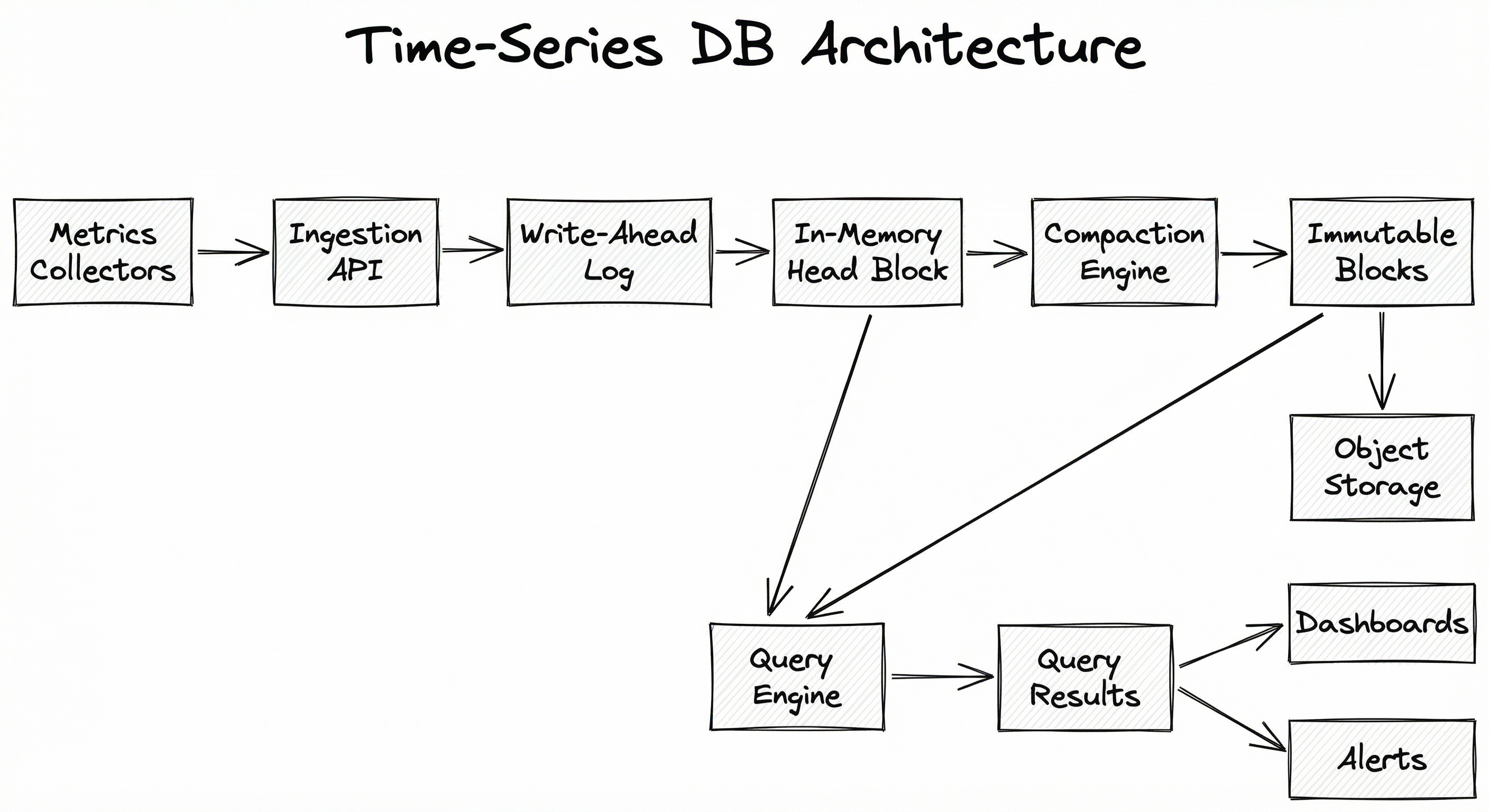
The write path is optimized for throughput: data flows through the WAL into an in-memory buffer, which periodically flushes to compressed on-disk blocks. The read path queries both the in-memory buffer (for recent data) and on-disk blocks (for historical data), merging results transparently. This dual-path architecture allows writes and reads to proceed largely without contention.
Key Components
Ingestion Layer
Accepts metric data via push (InfluxDB line protocol, OpenTelemetry, remote write) or pull (Prometheus scraping) protocols. Validates data format, assigns internal series IDs based on label sets, and routes samples to the WAL. Must handle burst traffic -- during model training, metric emission rates can spike 10-100x.
Write-Ahead Log (WAL)
Durably records every incoming sample before it is applied to the in-memory buffer. In the event of a crash, the WAL is replayed to recover un-flushed data. Prometheus uses a segmented WAL with configurable segment size; InfluxDB 3 uses Apache Parquet files as the WAL equivalent.
In-Memory Buffer (Head Block)
Stores the most recent time window of data (typically 1-4 hours) in memory for fast writes and queries. Prometheus calls this the head block; InfluxDB calls it the cache. Data here is uncompressed or lightly compressed for write speed. This is the primary source for real-time dashboards and alerts.
Compaction Engine
Periodically merges and compresses in-memory data into immutable, time-partitioned blocks on disk. Applies delta-of-delta timestamp compression and XOR value compression (Gorilla encoding). Also merges small blocks into larger ones to reduce file count and improve query efficiency. Compaction runs in the background to avoid blocking writes.
Storage Backend
Persists compressed blocks to local disk, network-attached storage, or object storage (S3, GCS, Azure Blob). Supports tiered storage: hot data on SSD, warm data on HDD, cold data on object storage. Retention policies automatically delete blocks older than the configured window.
Query Engine
Executes time-range queries using domain-specific languages (PromQL, SQL with time extensions, Flux, InfluxQL). Supports aggregation functions (rate, increase, histogram_quantile, moving_average), downsampled views, and label-based filtering. Queries span both the in-memory head block and on-disk blocks transparently.
Index (Inverted Index / Tag Index)
Maps label key-value pairs to series IDs for fast label-based lookups. Prometheus uses an in-memory inverted index; TimescaleDB leverages PostgreSQL B-tree indices on hypertable dimensions. High-cardinality label values (e.g., user_id) can bloat this index and degrade performance.
Data Flow
Write Path: Metric samples arrive via the ingestion API (push or pull) -> written to the WAL for durability -> applied to the in-memory head block -> periodically flushed and compressed into immutable on-disk blocks by the compaction engine -> oldest blocks pruned by retention policy.
Read Path: A time-range query enters the query engine -> the engine identifies which blocks (in-memory and on-disk) overlap the requested time range -> each block is scanned in parallel -> results are merged, aggregated, and returned to the caller (Grafana dashboard, alerting rule, or drift detection pipeline).
Downsampling Path: Continuous aggregate queries (TimescaleDB) or recording rules (Prometheus) periodically compute coarser-grained rollups from raw data -> rollups are stored as new time series -> raw data beyond the retention window is dropped, but rollups persist for long-term trend analysis.
The separation of hot (in-memory) and cold (on-disk) tiers ensures that real-time alerting queries hit fast in-memory data, while historical trend analysis queries efficiently scan compressed blocks without impacting write throughput.
A directed flow diagram showing: Metrics Collectors feed into an Ingestion API, which writes to a Write-Ahead Log, then to an In-Memory Buffer (Head Block). The Compaction Engine reads from the Head Block and produces Immutable Compressed Blocks stored on Disk or Object Storage. A Query Engine reads from both the Head Block and the Compressed Blocks to produce Query Results for dashboards, alerts, and drift detection.
How to Implement
Three Implementation Approaches
Implementation patterns for ML metrics storage fall into three categories:
Option A: Prometheus + VictoriaMetrics/Thanos -- Pull-based metrics collection with Prometheus, long-term storage via VictoriaMetrics or Thanos/Grafana Mimir. This is the most common stack for Kubernetes-native ML platforms. Zerodha runs this exact stack, storing 56 billion data points in their VictoriaMetrics cluster.
Option B: InfluxDB / QuestDB -- Push-based ingestion with a dedicated TSDB. Best for custom ML metrics pipelines where you control the emission format. InfluxDB 3 (written in Rust with Apache Arrow) can ingest millions of writes per second with sub-10ms lookups.
Option C: TimescaleDB (PostgreSQL extension) -- SQL-native time-series with continuous aggregates. Ideal when your team already uses PostgreSQL and wants to avoid introducing a new database technology. Full SQL support means you can join metrics with metadata tables.
The right choice depends on your existing infrastructure, team expertise, and scale. For a startup in Bengaluru building their first ML monitoring pipeline, Prometheus + Grafana is the fastest path to value (free, well-documented, massive ecosystem). For a large-scale platform processing 100K+ metrics per second, VictoriaMetrics or QuestDB provides the throughput headroom.
Cost Note: A VictoriaMetrics single-node instance handling 500K samples/sec runs comfortably on a 16-core, 64 GB VM -- roughly 0.002 per MB of writes. TimescaleDB Cloud starts at $29/month (~INR 2,400/month) for the smallest instance. Self-hosted Prometheus is free but requires operational investment for long-term storage.
from influxdb_client_3 import InfluxDBClient3
import pandas as pd
import time

# Initialize client
client = InfluxDBClient3(
    host="https://us-east-1-1.aws.cloud2.influxdata.com",
    token="YOUR_API_TOKEN",
    org="ml-team",
    database="ml_metrics"
)

# Write training metrics using line protocol
def log_training_step(epoch, step, loss, accuracy, lr, model_name):
    """Log a single training step's metrics to InfluxDB."""
    record = (
        f"training_metrics,model={model_name},stage=train "
        f"loss={loss},accuracy={accuracy},learning_rate={lr},"
        f"epoch={epoch}i,step={step}i {int(time.time_ns())}"
    )
    client.write(record=record)

# Simulate logging during training
for epoch in range(10):
    for step in range(100):
        log_training_step(
            epoch=epoch, step=step,
            loss=2.5 / (epoch + 1) + 0.01 * step,
            accuracy=0.5 + 0.05 * epoch,
            lr=0.001 * (0.95 ** epoch),
            model_name="bert-classifier-v3"
        )

# Query: average loss per epoch for the last 24 hours
query = """
SELECT
    epoch,
    AVG(loss) AS avg_loss,
    AVG(accuracy) AS avg_accuracy,
    MIN(learning_rate) AS lr
FROM training_metrics
WHERE time > now() - INTERVAL '24 hours'
    AND model = 'bert-classifier-v3'
GROUP BY epoch
ORDER BY epoch
"""
df = client.query(query=query, language="sql", mode="pandas")
print(df)
This example demonstrates writing ML training metrics to InfluxDB 3 using the line protocol format and querying them with SQL. The line protocol format is measurement,tag1=val1 field1=val1,field2=val2 timestamp -- tags are indexed (for filtering by model name, stage), fields store the actual metric values. InfluxDB 3 uses Apache Arrow and DataFusion under the hood, so SQL queries execute efficiently over columnar data.
-- Create a hypertable for inference metrics
CREATE TABLE inference_metrics (
    time        TIMESTAMPTZ NOT NULL,
    model_name  TEXT NOT NULL,
    endpoint    TEXT NOT NULL,
    latency_ms  DOUBLE PRECISION,
    confidence  DOUBLE PRECISION,
    prediction  TEXT,
    is_drift    BOOLEAN DEFAULT FALSE
);

SELECT create_hypertable('inference_metrics', by_range('time'));

-- Create an index on model_name for fast filtered queries
CREATE INDEX idx_model_time ON inference_metrics (model_name, time DESC);

-- Continuous aggregate: 5-minute rollups per model
CREATE MATERIALIZED VIEW inference_5min
WITH (timescaledb.continuous) AS
SELECT
    time_bucket('5 minutes', time) AS bucket,
    model_name,
    COUNT(*) AS request_count,
    AVG(latency_ms) AS avg_latency,
    percentile_cont(0.99) WITHIN GROUP (ORDER BY latency_ms) AS p99_latency,
    AVG(confidence) AS avg_confidence,
    STDDEV(confidence) AS stddev_confidence,
    SUM(CASE WHEN is_drift THEN 1 ELSE 0 END)::FLOAT / COUNT(*) AS drift_rate
WITH NO DATA;

-- Add a refresh policy: refresh every 5 minutes, covering the last 30 minutes
SELECT add_continuous_aggregate_policy('inference_5min',
    start_offset => INTERVAL '30 minutes',
    end_offset => INTERVAL '5 minutes',
    schedule_interval => INTERVAL '5 minutes'
);

-- Retention policy: keep raw data for 7 days, aggregates for 1 year
SELECT add_retention_policy('inference_metrics', INTERVAL '7 days');
SELECT add_retention_policy('inference_5min', INTERVAL '365 days');

-- Query: detect latency spikes in the last hour
SELECT
    bucket,
    model_name,
    avg_latency,
    p99_latency,
    drift_rate
FROM inference_5min
WHERE bucket > NOW() - INTERVAL '1 hour'
    AND p99_latency > 200
ORDER BY p99_latency DESC;
TimescaleDB extends PostgreSQL with hypertables (automatically partitioned tables) and continuous aggregates (incrementally maintained materialized views). This example creates a hypertable for inference metrics, a continuous aggregate that computes 5-minute rollups including P99 latency and drift rate, and retention policies that keep raw data for 7 days but aggregates for a year. This pattern -- high-resolution recent data with progressively coarser historical data -- is the standard approach for ML monitoring at scale.
from prometheus_client import (
    start_http_server, Histogram, Counter, Gauge, Summary
)
import time
import random

# Define ML-specific metrics
INFERENCE_LATENCY = Histogram(
    'ml_inference_latency_seconds',
    'Time spent processing inference request',
    ['model_name', 'model_version'],
    buckets=[0.01, 0.025, 0.05, 0.1, 0.25, 0.5, 1.0, 2.5]
)

PREDICTION_CONFIDENCE = Summary(
    'ml_prediction_confidence',
    'Confidence score of model predictions',
    ['model_name']
)

PREDICTION_COUNT = Counter(
    'ml_predictions_total',
    'Total number of predictions made',
    ['model_name', 'predicted_class']
)

MODEL_DRIFT_SCORE = Gauge(
    'ml_model_drift_score',
    'Current drift score (PSI or KL divergence)',
    ['model_name', 'feature_name']
)

GPU_MEMORY_USAGE = Gauge(
    'ml_gpu_memory_bytes',
    'GPU memory usage in bytes',
    ['gpu_id', 'model_name']
)

def simulate_inference():
    """Simulate an ML inference with metric instrumentation."""
    model = "fraud-detector-v2"
    version = "2.1.0"

    # Time the inference
    with INFERENCE_LATENCY.labels(
        model_name=model, model_version=version
    ).time():
        # Simulate model inference
        time.sleep(random.uniform(0.01, 0.15))
        confidence = random.gauss(0.85, 0.1)
        predicted_class = "fraud" if confidence > 0.7 else "legitimate"

    # Record prediction metrics
    PREDICTION_CONFIDENCE.labels(model_name=model).observe(confidence)
    PREDICTION_COUNT.labels(
        model_name=model, predicted_class=predicted_class
    ).inc()

    # Update drift score (computed externally, e.g., by Evidently)
    MODEL_DRIFT_SCORE.labels(
        model_name=model, feature_name="transaction_amount"
    ).set(random.uniform(0.01, 0.3))

    # GPU memory (from nvidia-smi or pynvml)
    GPU_MEMORY_USAGE.labels(
        gpu_id="0", model_name=model
    ).set(random.randint(2_000_000_000, 8_000_000_000))

if __name__ == '__main__':
    # Start Prometheus metrics server on port 8000
    start_http_server(8000)
    print("Metrics server started on :8000/metrics")
    while True:
        simulate_inference()
        time.sleep(0.1)  # ~10 inferences/sec
This example creates a Prometheus exporter for ML inference metrics. Prometheus pulls (scrapes) these metrics at a configured interval (typically 15-30 seconds). The key metric types are: Histogram for latency distributions (enables P50/P99 calculations via histogram_quantile), Counter for monotonically increasing totals, Gauge for point-in-time values like drift scores, and Summary for client-side quantile calculation. This exporter would be scraped by Prometheus and visualized in Grafana.
import requests
import json
from datetime import datetime, timedelta

VICTORIA_METRICS_URL = "http://victoriametrics:8428"

def import_metrics_bulk(metrics: list[dict]):
    """Bulk import metrics to VictoriaMetrics via JSON import API."""
    payload = ""
    for m in metrics:
        payload += json.dumps({
            "metric": {
                "__name__": m["name"],
                "model": m.get("model", "unknown"),
                "environment": m.get("env", "production")
            },
            "values": m["values"],
            "timestamps": m["timestamps"]
        }) + "\n"

    resp = requests.post(
        f"{VICTORIA_METRICS_URL}/api/v1/import",
        data=payload,
        headers={"Content-Type": "application/json"}
    )
    resp.raise_for_status()
    print(f"Imported {len(metrics)} series successfully")

def query_model_latency_trend(model_name: str, hours: int = 24):
    """Query P99 inference latency trend using PromQL."""
    query = (
        f'histogram_quantile(0.99, '
        f'rate(ml_inference_latency_seconds_bucket{{model_name="{model_name}"}}[5m]))'
    )
    end = datetime.utcnow()
    start = end - timedelta(hours=hours)

    resp = requests.get(
        f"{VICTORIA_METRICS_URL}/api/v1/query_range",
        params={
            "query": query,
            "start": start.isoformat() + "Z",
            "end": end.isoformat() + "Z",
            "step": "5m"
        }
    )
    data = resp.json()
    for result in data.get("data", {}).get("result", []):
        print(f"Labels: {result['metric']}")
        for ts, val in result["values"]:
            print(f"  {datetime.fromtimestamp(ts)}: {float(val)*1000:.1f}ms")

def detect_latency_anomaly(model_name: str, threshold_multiplier: float = 2.0):
    """Detect if current P99 latency exceeds 2x the 7-day average."""
    current_query = (
        f'histogram_quantile(0.99, '
        f'rate(ml_inference_latency_seconds_bucket{{model_name="{model_name}"}}[5m]))'
    )
    baseline_query = (
        f'avg_over_time('
        f'histogram_quantile(0.99, '
        f'rate(ml_inference_latency_seconds_bucket{{model_name="{model_name}"}}[5m]))[7d:1h])'
    )

    current = requests.get(
        f"{VICTORIA_METRICS_URL}/api/v1/query",
        params={"query": current_query}
    ).json()
    baseline = requests.get(
        f"{VICTORIA_METRICS_URL}/api/v1/query",
        params={"query": baseline_query}
    ).json()

    current_val = float(current["data"]["result"][0]["value"][1])
    baseline_val = float(baseline["data"]["result"][0]["value"][1])

    if current_val > baseline_val * threshold_multiplier:
        print(f"ANOMALY: P99 latency {current_val*1000:.1f}ms "
              f"exceeds {threshold_multiplier}x baseline {baseline_val*1000:.1f}ms")
        return True
    return False

# Usage
query_model_latency_trend("fraud-detector-v2", hours=6)
detect_latency_anomaly("fraud-detector-v2")
VictoriaMetrics is a drop-in replacement for Prometheus with superior compression (up to 70x vs TimescaleDB) and lower memory usage (10x less than InfluxDB). This example demonstrates bulk metric import and PromQL-based queries for ML monitoring, including a latency anomaly detection function that compares current P99 to a 7-day rolling baseline. VictoriaMetrics supports the full Prometheus remote write and query APIs, so it integrates seamlessly with existing Prometheus exporters and Grafana dashboards.
# Prometheus configuration for ML metrics scraping
global:
  scrape_interval: 15s
  evaluation_interval: 15s
  external_labels:
    cluster: ml-prod-ap-south-1
    environment: production

# Remote write to VictoriaMetrics for long-term storage
remote_write:
  - url: http://victoriametrics:8428/api/v1/write
    queue_config:
      max_samples_per_send: 10000
      batch_send_deadline: 5s
      max_shards: 30

scrape_configs:
  - job_name: ml-inference-service
    scrape_interval: 15s
    metrics_path: /metrics
    kubernetes_sd_configs:
      - role: pod
    relabel_configs:
      - source_labels: [__meta_kubernetes_pod_label_app]
        regex: ml-inference-.*
        action: keep
      - source_labels: [__meta_kubernetes_pod_label_model]
        target_label: model_name

  - job_name: ml-training-jobs
    scrape_interval: 30s
    kubernetes_sd_configs:
      - role: pod
    relabel_configs:
      - source_labels: [__meta_kubernetes_pod_label_app]
        regex: training-.*
        action: keep

# Recording rules for pre-computed ML aggregates
rule_files:
  - /etc/prometheus/ml_recording_rules.yml

# Alerting rules for model health
alerting:
  alertmanagers:
    - static_configs:
        - targets: ['alertmanager:9093']
Common Implementation Mistakes
- ●
High-cardinality label explosion: Using unbounded labels like
user_id,request_id, ortrace_idas metric labels creates millions of unique time series, causing the inverted index to balloon and queries to slow to a crawl. Labels should have bounded, low cardinality (tens to thousands of unique values, not millions). Use a separate tracing system for high-cardinality identifiers. - ●
Missing retention policies: Without explicit retention, TSDB storage grows unboundedly. A system ingesting 100K samples/sec generates ~8.6 billion samples/day. Even with 2-byte compression, that is ~17 GB/day of compressed data. After a year without retention, you are looking at 6+ TB and degrading query performance.
- ●
Scrape interval too aggressive: Setting Prometheus scrape interval to 1 second when 15-30 seconds would suffice multiplies storage by 15-30x and increases CPU load on both the exporter and Prometheus. For ML metrics, 15-second granularity is sufficient for most monitoring use cases; sub-second metrics belong in a different collection path.
- ●
Not using continuous aggregates or recording rules: Querying raw, high-resolution data for dashboard panels that display hourly or daily trends is extremely wasteful. Pre-compute these aggregates using Prometheus recording rules or TimescaleDB continuous aggregates to keep dashboard queries fast.
- ●
Ignoring timezone and clock skew: In distributed ML systems, metric timestamps from different nodes may be skewed by seconds or even minutes. This causes misleading spikes and gaps in dashboards. Use NTP synchronization across all nodes and configure the TSDB to handle out-of-order writes (Prometheus v2.39+ supports this natively).
When Should You Use This?
Use When
Your ML system generates continuous streams of timestamped metrics (training loss, inference latency, prediction confidence, feature distributions) that need to be stored and queried over time ranges
You need real-time dashboards and alerting on model health metrics -- P99 latency, throughput, error rates, drift scores -- with sub-second query response times
You require automatic data lifecycle management: high-resolution recent data with progressive downsampling and eventual deletion of old raw data
Your monitoring workload is write-heavy (append-only) with time-range-based read patterns -- the classic TSDB sweet spot
You need to store and query metrics at high cardinality (thousands of unique model/endpoint/region combinations) with efficient label-based filtering
You want to detect anomalies, trends, and drift by comparing current metric values against historical baselines using built-in temporal functions
You are building a Kubernetes-native ML platform and need Prometheus-compatible metrics collection with long-term storage
Avoid When
Your data does not have a natural time dimension or your queries are not primarily time-range-based -- use a relational or document database instead
You need complex joins between metrics and non-temporal data (user profiles, experiment metadata) -- use a data warehouse like BigQuery or Snowflake, or TimescaleDB if you need both SQL joins and time-series features
Your use case requires strong ACID transactions with rollback capability -- most TSDBs are append-only and do not support UPDATE or DELETE on individual records
You are storing ML artifacts (model weights, training datasets, evaluation reports) rather than numeric metrics -- use an object store or artifact registry
Your metric cardinality is extremely low (<100 unique series) and data volume is small -- a simple CSV file, SQLite, or even a Python dictionary may be simpler and sufficient
You need full-text search over log messages alongside metrics -- consider a unified observability platform like Elasticsearch/OpenSearch or Grafana Loki for logs combined with a TSDB for metrics
Key Tradeoffs
The Fundamental Tradeoff: Write Throughput vs. Query Flexibility
TSDBs optimized for maximum write throughput (Prometheus, VictoriaMetrics) typically use domain-specific query languages (PromQL, MetricsQL) with limited expressiveness -- no joins, no subqueries, no window functions beyond what is built in. TSDBs that offer SQL (TimescaleDB, QuestDB) provide richer query capabilities but may sacrifice some write performance.
For ML monitoring, this tradeoff matters because drift detection queries can be surprisingly complex: comparing current feature distributions against a baseline window, computing KL divergence or PSI across multiple features, and correlating metric changes with model deployment events. If your drift detection runs as offline batch jobs, PromQL is fine. If you need ad-hoc, SQL-based analysis, TimescaleDB or QuestDB is a better fit.
The Second Axis: Operational Simplicity vs. Scale
| Dimension | Prometheus (Single Node) | VictoriaMetrics | TimescaleDB | InfluxDB 3 | QuestDB |
|---|---|---|---|---|---|
| Max Ingestion | ~500K samples/s | ~2M samples/s | ~500K rows/s | ~3M rows/s | ~11M rows/s |
| Compression | ~1.3 bytes/sample | ~0.4 bytes/sample | ~8 bytes/sample | ~2 bytes/sample | ~4 bytes/sample |
| Query Language | PromQL | PromQL/MetricsQL | SQL | SQL/InfluxQL | SQL |
| Operational Complexity | Low (single binary) | Low-Medium | Low (PostgreSQL) | Medium | Low (single binary) |
| Long-Term Storage | Limited (local disk) | Object storage | PostgreSQL storage | Object storage | Local disk |
| Cost (self-hosted, ~1M series) | Free + ~$200/mo VM | Free + ~$400/mo VM | Free + ~$300/mo VM | Free/Cloud ~$500/mo | Free + ~$250/mo VM |
Cost Considerations for Indian Teams
Self-hosted Prometheus + VictoriaMetrics on a 16-core, 64 GB EC2 instance in Mumbai (ap-south-1) costs approximately 29/month (~INR 2,400/month) for development. InfluxDB Cloud Serverless charges per-usage, which can be cost-effective for bursty workloads but unpredictable for steady, high-throughput ML metrics.
Rule of Thumb: Start with Prometheus + Grafana for metrics collection and visualization. When you outgrow single-node Prometheus (typically at >1M active time series or >2 weeks retention), add VictoriaMetrics as long-term storage. Only adopt TimescaleDB or QuestDB if you need SQL-based analytics on your metrics data.
Alternatives & Comparisons
A data lake stores raw, immutable data at very low cost but lacks the real-time query performance and built-in temporal functions of a TSDB. Use a data lake for long-term archival of ML metrics (months to years) and batch analytics; use a TSDB for real-time monitoring and alerting (hours to weeks). Many production systems use both: TSDB for hot data, data lake for cold data.
Streaming platforms transport and process metrics in real-time but do not store them durably for historical queries. A TSDB is the persistent storage layer that receives data from streaming pipelines. Use Kafka/Flink for real-time feature computation and event routing; use a TSDB for durable storage and time-range queries. They are complementary, not competing.
Metrics collectors gather and route metric data but do not store it. The TSDB is the storage backend that collectors write to. OpenTelemetry Collector can fan-out metrics to multiple TSDBs simultaneously. They are always used together: the collector is the plumbing, the TSDB is the tank.
Drift detection computes statistical tests on feature and prediction distributions but needs a storage backend for the metric time series it produces (PSI scores, KL divergence values over time). The TSDB stores the drift scores; the drift detection service computes them. They form a tight feedback loop: drift service writes scores to the TSDB, dashboards and alerts read from the TSDB.
Pros, Cons & Tradeoffs
Advantages
Extreme write throughput: Modern TSDBs handle 1-11 million writes per second on a single node, enabling real-time ingestion of ML metrics at scale without batching delays or back-pressure concerns.
Exceptional compression: Gorilla-style delta-of-delta and XOR encoding achieves 10-70x compression ratios on typical metrics data, reducing storage costs dramatically. VictoriaMetrics stores up to 70x more data points than TimescaleDB in the same storage space.
Built-in temporal operations: Functions like
rate(),increase(),histogram_quantile(),avg_over_time(), and moving window aggregations are first-class operations, not bolted-on extensions. This makes drift detection and anomaly queries concise and fast.Automatic data lifecycle management: Retention policies and continuous aggregates/recording rules handle the transition from high-resolution recent data to low-resolution historical data automatically. You set the policy once and the TSDB manages it forever.
Native Grafana integration: All major TSDBs integrate with Grafana out of the box, providing rich visualization, alerting, and dashboarding without custom UI work. This accelerates time-to-insight for ML monitoring.
Ecosystem maturity: Prometheus has 1,000+ exporters, OpenTelemetry supports all major TSDBs, and every cloud provider offers managed TSDB services. You are never building from scratch.
Disadvantages
High-cardinality limitations: Most TSDBs degrade significantly when cardinality exceeds 1-10 million unique series. This is a real constraint for ML systems that want to track per-user or per-request metrics. Workaround: use exemplars or sampling instead of per-request labels.
Limited query expressiveness: PromQL and InfluxQL lack joins, subqueries, and complex aggregations that SQL provides. Drift detection queries that require comparing distributions across windows can be awkward. TimescaleDB and QuestDB address this with full SQL, but sacrifice some write performance.
Append-only semantics: You cannot easily update or delete individual data points. If you log incorrect metric values (e.g., due to a bug in your exporter), you cannot surgically fix them. You typically have to drop and re-ingest the affected time range.
Operational complexity at scale: Running a highly available, multi-node TSDB cluster (VictoriaMetrics cluster, Milvus, Thanos) requires expertise in replication, sharding, compaction tuning, and capacity planning. This is non-trivial for a small team.
Not a general-purpose database: TSDBs cannot replace your relational database for experiment tracking, model registry, or user management. They solve one problem extremely well but you still need other storage systems alongside them.
Failure Modes & Debugging
Cardinality explosion
Cause
Adding a high-cardinality label (e.g., user_id, request_id, session_id) to metrics creates millions of unique time series. This is the single most common TSDB failure in ML systems, often caused by well-intentioned engineers who want per-request tracking.
Symptoms
Memory usage spikes dramatically, the inverted index grows unboundedly, query latency degrades from milliseconds to seconds or minutes, and eventually the TSDB OOMs or becomes unresponsive. In Prometheus, you will see prometheus_tsdb_head_series increasing without bound.
Mitigation
Enforce label cardinality limits at the collection layer. Use relabeling rules in Prometheus to drop high-cardinality labels before ingestion. For per-request tracing, use a separate tracing system (Jaeger, Tempo) rather than metrics labels. Set alerts on prometheus_tsdb_head_series to catch explosions early.
Retention policy misconfiguration
Cause
Raw data retention set too long (or not set at all), or continuous aggregates not configured, leading to unbounded storage growth and progressively slower queries as the database scans increasingly large time ranges.
Symptoms
Disk usage grows linearly without plateau, queries over long time ranges time out, compaction falls behind, and eventually the disk fills up causing write failures. In a cloud environment, you see unexpectedly large storage bills.
Mitigation
Always configure explicit retention policies from day one. Implement a tiered strategy: raw data for 7-30 days, 5-minute aggregates for 90 days, hourly aggregates for 1-2 years. Use continuous aggregates (TimescaleDB) or recording rules (Prometheus) to pre-compute long-term rollups before raw data is dropped.
Write amplification during compaction
Cause
The compaction engine rewrites and merges blocks in the background. Under heavy write load, compaction can fall behind, leading to an excessive number of small blocks that degrade query performance and increase I/O.
Symptoms
Increasing number of on-disk blocks, rising query latency over time, high disk I/O utilization even during low-traffic periods, and eventually write failures if compaction cannot keep up. Prometheus logs will show compact warnings.
Mitigation
Provision sufficient I/O bandwidth (use SSDs, not HDDs). Tune compaction parameters: increase compaction concurrency, adjust block time ranges. For Prometheus, ensure the --storage.tsdb.max-block-duration is appropriate for your data volume. Monitor compaction lag as a key operational metric.
Clock skew causing data gaps and duplicates
Cause
In distributed ML systems, metric timestamps from different nodes are not synchronized. Nodes with fast clocks produce timestamps in the "future" (relative to the TSDB), while slow clocks produce timestamps that appear as "late" or "out-of-order" writes.
Symptoms
Dashboards show intermittent gaps or spikes in metrics. Rate calculations produce negative values (impossible for counters). Alerting rules fire spuriously. Data appears duplicated when queried at high resolution.
Mitigation
Deploy NTP synchronization across all nodes (chrony is the modern standard). Enable out-of-order ingestion in Prometheus (available since v2.39 with --storage.tsdb.allow-overlapping-compaction). For InfluxDB and VictoriaMetrics, out-of-order writes are handled natively.
Query of death (resource-exhausting query)
Cause
A user or automated dashboard runs a query that scans too many time series over too large a time range without sufficient aggregation. For example, rate(http_requests_total[30d]) on 100K series would attempt to load and process billions of samples.
Symptoms
The TSDB process consumes all available memory and CPU, other queries time out, dashboards go blank for all users, and in severe cases the TSDB crashes. This is often caused by Grafana dashboards with overly broad default time ranges.
Mitigation
Set query limits: --query.max-samples in Prometheus, maxPointsPerTimeseries in VictoriaMetrics. Use recording rules to pre-compute expensive aggregations. Configure Grafana dashboard default time ranges to reasonable windows (1h or 6h, not 30d). Implement query cost estimation and rejection for queries exceeding resource budgets.
Metric staleness after model redeployment
Cause
When an ML model is redeployed, old metric series (with the previous version label) stop receiving updates but remain in the TSDB head block. The TSDB marks them as "stale" after a timeout, but during the staleness window, dashboards may show misleading data.
Symptoms
After redeployment, dashboards show a brief period where both old and new model versions appear active. Aggregation queries double-count during the overlap. Alert rules may fire or fail to fire during the transition.
Mitigation
Use Prometheus staleness handling (default 5-minute staleness timeout). Ensure your metric labels include model_version so old and new series are distinct. Configure dashboards to filter by the active model version. Consider using the up metric or a custom deployment timestamp metric to gate visibility.
Placement in an ML System
Where Does It Sit in the Pipeline?
In an ML monitoring pipeline, the time-series database sits directly downstream of metrics collectors (Prometheus exporters, OpenTelemetry collectors, StatsD agents) and directly upstream of visualization (Grafana dashboards), alerting (Alertmanager, PagerDuty), and analytical systems (drift detection, anomaly detection).
The TSDB is the central nervous system of ML observability. It stores the vital signs of every model in production: latency distributions, throughput rates, error counts, prediction confidence trends, feature drift scores, and resource utilization. Without it, you are flying blind.
For training pipelines, the TSDB stores epoch-level metrics (loss, accuracy, learning rate) that enable training curve visualization and early stopping decisions. MLflow and Weights & Biases use TSDBs internally for this purpose.
For inference pipelines, the TSDB stores per-endpoint, per-model metrics that feed into SLO (service level objective) tracking and automated rollback decisions. If P99 latency exceeds 200ms or drift score exceeds a threshold, the alerting system (reading from the TSDB) triggers a notification or automated action.
Key Insight: The time-series database determines how quickly you can detect and respond to production ML issues. A well-configured TSDB with appropriate retention policies, continuous aggregates, and alerting rules is the difference between catching model degradation in minutes versus discovering it days later through user complaints.
Pipeline Stage
Monitoring / Observability
Upstream
- metrics-collector
- streaming-data-source
- model-serving
Downstream
- drift-detection
- alerting-system
- dashboard-visualization
Scaling Bottlenecks
The primary bottleneck is cardinality -- the number of unique time series. Each unique combination of metric name and label values creates a distinct series that requires memory for the in-memory index and head block. At 10 million active series, most single-node TSDBs start to struggle.
The second bottleneck is ingestion rate. Prometheus on a single node tops out at roughly 500K-1M samples/sec. VictoriaMetrics pushes to 2M+. QuestDB leads with 4-11M rows/sec. Beyond these limits, you need sharding across multiple nodes.
Some concrete numbers for ML workloads: a platform serving 50 ML models, each emitting 20 metrics with 5 label dimensions, scraped every 15 seconds, generates approximately unique series and samples/minute -- well within single-node capacity. Scale to 5,000 models with high-cardinality labels and you are at 5M+ series, requiring a distributed setup (VictoriaMetrics cluster, Thanos, or Grafana Mimir).
Production Case Studies
Uber built M3, an open-source metrics platform centered on M3DB, a custom distributed TSDB. M3 stores 6.6 billion time series, aggregates 500 million metrics per second, and persists 20 million metrics per second globally. M3DB uses an optimized version of Gorilla's TSZ compression (called M3TSZ) and columnar storage for memory locality. The platform replaced Uber's legacy Graphite-based system, which could not handle the scale of their ML and microservices monitoring.
M3DB achieved an 11x compression ratio over the original Gorilla encoding, reduced infrastructure costs significantly by bringing replication factor back to 3, and the query engine benchmarks at 2,500 queries per second. Uber uses M3 to monitor ML model performance across their pricing, ETA prediction, and fraud detection systems.
Netflix built Atlas, an in-memory dimensional time-series database that serves as their primary telemetry platform. Atlas ingests multiple billions of time series per day, supports arbitrary key-value label dimensions, and retains the last two weeks of data in memory for real-time querying. Netflix uses Atlas to monitor their recommendation ML models, content delivery algorithms, and streaming quality metrics. The system handles 20x more queries than when originally launched, with platform teams programmatically generating alerts on behalf of their users.
Atlas processes over 1 billion metrics per minute and enables real-time operational insight across all of Netflix's services. The dimensional data model allows engineers to slice metrics by any combination of labels without pre-defining aggregation hierarchies.
Zerodha, India's largest retail stock investment platform handling 8 million trades per day, uses Prometheus for metrics collection and VictoriaMetrics for long-term storage. Their monitoring stack tracks trade execution latency, order placement metrics, and system health across a hybrid infrastructure of VMs, containers, and Kubernetes clusters. Zerodha stores approximately 56 billion time-series data points in their VictoriaMetrics cluster, ingesting tens of thousands of metrics every second.
Prometheus + VictoriaMetrics provided centralized, uniform monitoring across Zerodha's complex financial infrastructure. The large ecosystem of existing Prometheus exporters enabled wide coverage quickly, critical for a regulated financial system where monitoring gaps can have legal and financial consequences.
Razorpay, processing millions of payment transactions monthly across hundreds of microservices and thousands of containers, implemented a unified observability platform with time-series metrics, traces, and logs. Their infrastructure spans several thousand nodes, and they use priority-based data tiering -- frequently searched metrics are indexed in hot storage for real-time queries, while less critical data moves to cost-effective cold storage.
The unified observability approach allowed Razorpay to correlate payment success rates with infrastructure metrics in real time, reducing mean time to detection (MTTD) for payment failures. This is critical for maintaining the trust of their merchant base across India.
Tooling & Ecosystem
The de facto standard for metrics collection in cloud-native environments. Pull-based model with powerful PromQL query language. Built-in alerting rules and Grafana integration. Ideal for Kubernetes-native ML platforms. Limitation: single-node only, limited long-term storage (typically 15-30 days).
High-performance, cost-effective monitoring solution compatible with Prometheus. Up to 10x lower memory than InfluxDB and 70x better compression than TimescaleDB. Supports both single-node and cluster modes. Drop-in replacement for Prometheus long-term storage via remote write. Used by Zerodha for storing 56 billion data points.
Purpose-built TSDB with push-based ingestion. InfluxDB 3 (rewritten in Rust with Apache Arrow, DataFusion, and Parquet) delivers millions of writes per second and sub-10ms lookups. Supports SQL, InfluxQL, and the line protocol for ingestion. Available as open-source (Core) and managed cloud service.
PostgreSQL extension for time-series data. Provides hypertables (auto-partitioned tables), continuous aggregates (incrementally maintained views), and retention policies -- all accessible via standard SQL. Best for teams already on PostgreSQL who need time-series capabilities without a new database. Supports complex analytical queries 3.4-71x faster than InfluxDB.
High-performance TSDB written in Java and C++. Benchmarks show 4-11 million rows/sec ingestion and 12-36x faster than InfluxDB 3 for ingestion, with 43-418x faster complex analytical queries. SQL-native with a web console. Excellent for high-throughput ML metrics pipelines.
The standard visualization and dashboarding platform for time-series data. Connects to all major TSDBs (Prometheus, InfluxDB, TimescaleDB, QuestDB, VictoriaMetrics) as data sources. Provides alerting, annotations, and templated dashboards. Essential companion to any TSDB in an ML monitoring stack.
Open-source, horizontally scalable long-term storage for Prometheus. Handles up to 1 billion active time series. Uses object storage (S3, GCS, Azure Blob) as the backend. Alternative to VictoriaMetrics and Thanos for scaling Prometheus beyond a single node.
Vendor-neutral telemetry pipeline that collects, processes, and exports metrics (and traces and logs) to multiple backends simultaneously. Acts as the glue between metric emitters and TSDBs. Supports Prometheus, OTLP, StatsD, and many other protocols.
Research & References
Pelkonen, Franklin, Teller, Cavallaro, Huang, Meza, Veeraraghavan (2015)VLDB 2015
Introduced delta-of-delta timestamp compression and XOR floating-point compression at Facebook, achieving 12x compression and 73x query latency reduction compared to HBase. The compression algorithms from this paper are now used in Prometheus, VictoriaMetrics, M3DB, and most modern TSDBs.
Netflix Technology Blog (2016)Netflix TechBlog
Describes Netflix's approach to scaling their time-series telemetry infrastructure, covering the challenges of dimensional data models, high cardinality, and the evolution from simple counters to rich, multi-dimensional metrics.
Liu, Chen, Wang, et al. (2024)arXiv preprint
Comprehensive decade-spanning review of time-series anomaly detection methods, covering statistical approaches, deep learning models, and hybrid techniques. Directly relevant to ML monitoring systems that store anomaly detection results in TSDBs.
Schmidl, Wenig, Papenbrock (2022)ACM Computing Surveys, 2024
Systematic survey of deep learning approaches for time-series anomaly detection, including autoencoders, GANs, and transformer-based methods. Provides benchmarks and evaluation metrics relevant to ML model monitoring pipelines.
Uber Engineering (2021)Uber Engineering Blog
Describes the engineering challenges and solutions for querying billions of high-cardinality time-series data points in Uber's M3 platform, including index optimization and query parallelization techniques.
Harel, Mannor, El-Yaniv, Crammer (2021)arXiv preprint
Proposes methods for real-time concept drift detection in streaming time-series data, directly applicable to ML model monitoring where feature distributions shift over time and need to be detected from TSDB-stored metrics.
Interview & Evaluation Perspective
Common Interview Questions
- ●
How would you design a monitoring system for 500 ML models in production, each emitting 30 metrics every 15 seconds?
- ●
What is the difference between Prometheus (pull-based) and InfluxDB (push-based) architectures? When would you choose each?
- ●
Explain cardinality in the context of time-series databases. Why is it the primary scaling concern?
- ●
How would you implement a data retention strategy that keeps high-resolution data for 7 days and hourly aggregates for 1 year?
- ●
Design a system that detects model drift using time-series metrics. What metrics would you store and how would you query them?
- ●
How does delta-of-delta compression work for timestamps? Why does it achieve such high compression ratios?
Key Points to Mention
- ●
Cardinality (number of unique time series) is the primary scaling dimension, not data volume. A system with 10M unique series is harder to handle than one with 1M series ingesting 10x more samples per series.
- ●
Gorilla compression (delta-of-delta for timestamps, XOR for values) achieves 10-12x compression on typical metrics data, with 96% of timestamps compressing to a single bit.
- ●
Prometheus uses a pull model (scrapes targets) which has advantages for service discovery and avoiding push storms, while InfluxDB/VictoriaMetrics support push which is better for short-lived training jobs.
- ●
Continuous aggregates (TimescaleDB) and recording rules (Prometheus) are essential for pre-computing expensive queries and enabling fast dashboards. Without them, every dashboard panel re-scans raw data.
- ●
Retention policies must be configured from day one -- not retrofitted. A tiered strategy (raw -> 5min -> hourly -> daily) is standard practice.
- ●
For ML-specific monitoring, the key metrics to store are: inference latency distribution (histogram), prediction confidence distribution, feature drift scores (PSI, KL divergence), throughput, error rates, and resource utilization (GPU memory, CPU).
Pitfalls to Avoid
- ●
Conflating time-series databases with general-purpose analytics databases -- TSDBs excel at temporal queries but are poor at joins, transactions, and non-temporal lookups.
- ●
Proposing per-request labels (user_id, request_id) in Prometheus metrics -- this causes cardinality explosion and is the most common mistake in TSDB design interviews.
- ●
Ignoring the cost of long-term retention: storing 1M series at 15-second intervals for 1 year produces ~2 trillion samples. Even at 1 byte/sample compressed, that is 2 TB of storage.
- ●
Assuming Prometheus can serve as long-term storage -- single-node Prometheus is designed for 15-30 days of local retention. For longer retention, you need VictoriaMetrics, Thanos, or Grafana Mimir.
Senior-Level Expectation
A senior candidate should discuss the full observability architecture: metric emission strategy (what to measure, at what granularity), collection pipeline (Prometheus vs. OpenTelemetry, push vs. pull), storage tier design (hot/warm/cold with concrete retention windows), query optimization (recording rules, continuous aggregates, query cost limits), alerting philosophy (symptom-based vs. cause-based alerts), and capacity planning (cardinality estimation, storage projections, cost modeling in INR/USD). They should be able to estimate that monitoring 500 models with 30 metrics each, 5 label dimensions, scraped every 15 seconds produces approximately 75,000 unique series and 300,000 samples/minute -- comfortably within single-node Prometheus capacity. They should also articulate why ML monitoring requires different metrics than traditional application monitoring (distribution-based metrics like histograms over point metrics like gauges, feature drift tracking, model version correlation).
Summary
Let's recap what we have covered:
-
A time-series database is a storage engine purpose-built for high-throughput ingestion, aggressive compression, and fast time-range queries over timestamped metric data. For ML systems, it is the backbone of monitoring and observability -- storing everything from inference latency distributions to feature drift scores to GPU utilization.
-
The core algorithms are delta-of-delta timestamp compression and XOR value encoding (from Facebook's Gorilla paper), achieving 10-12x compression with 96% of timestamps compressing to a single bit. This enables storing billions of data points on modest hardware.
-
Cardinality (the number of unique time series) is the primary scaling dimension, not data volume. High-cardinality labels like
user_idorrequest_idcause index explosion and are the most common TSDB failure mode. Always use bounded, low-cardinality labels for metrics. -
The production stack for most ML teams is Prometheus for metrics collection + VictoriaMetrics or Grafana Mimir for long-term storage + Grafana for visualization and alerting. Teams needing SQL analytics on metrics should consider TimescaleDB or QuestDB.
-
Retention policies and continuous aggregates are non-negotiable. The standard pattern is: raw data for 7-30 days, 5-minute aggregates for 90 days, hourly aggregates for 1+ year. Without this tiered strategy, storage grows unboundedly and queries degrade.
-
Real-world deployments validate the approach: Uber's M3 stores 6.6 billion series, Netflix's Atlas ingests 1 billion metrics per minute, and Zerodha monitors 8 million daily trades with 56 billion data points in VictoriaMetrics.
The time-series database is the central nervous system of ML observability. It stores the vital signs of every model in production and determines how quickly you can detect and respond to degradation. Get this layer right, and everything downstream -- dashboards, alerts, drift detection, automated rollbacks -- becomes dramatically easier.