Batch Data Source in Machine Learning
A batch data source is the foundational entry point for historical data flowing into an ML pipeline. It reads data from databases, data lakes, flat files, or warehouses in discrete, scheduled chunks -- not continuously, but at defined intervals or on-demand triggers.
In every production ML system, there's a moment where raw historical data needs to cross the boundary from "stored somewhere" to "available for training or feature engineering." That boundary crossing is what a batch data source handles. It's the extract in ETL, the first node in your Spark DAG, the pd.read_parquet() call that kicks off your notebook.
Why does this deserve its own block in a system design? Because getting data into a pipeline reliably, efficiently, and reproducibly is harder than it looks. You're dealing with terabyte-scale reads, evolving schemas, network partitions to remote databases, format mismatches, and the ever-present need to know exactly which version of the data produced a given model. Flipkart processes 10+ TB of raw text data daily; Zerodha runs batch PnL calculations over 100 million transactional records. At these scales, a naive SELECT * is not a strategy -- it's a disaster.
Batch data sources are the quiet workhorses of ML infrastructure. They lack the glamour of model architectures or the urgency of real-time serving, but without a robust batch ingestion layer, nothing downstream works. Garbage in, garbage out -- and the "in" starts right here.
Concept Snapshot
- What It Is
- A system component that reads historical data from databases, data lakes, or file systems in discrete scheduled or triggered batches to feed ML training, feature engineering, or evaluation pipelines.
- Category
- Data Ingestion
- Complexity
- Intermediate
- Inputs / Outputs
- Inputs: connection strings, file paths, SQL queries, partition filters, schema definitions. Outputs: structured DataFrames, datasets, or record batches ready for downstream processing.
- System Placement
- Sits at the very beginning of an ML pipeline, upstream of data validation, cleaning, transformation, and feature engineering stages.
- Also Known As
- batch data reader, offline data source, historical data loader, batch ingestion layer, data extractor, ETL source connector
- Typical Users
- Data Engineers, ML Engineers, Data Scientists, MLOps Engineers, Analytics Engineers
- Prerequisites
- SQL and database fundamentals, File formats (Parquet, CSV, JSON, Avro, ORC), Distributed computing basics (Spark, MapReduce), Data lake concepts (S3, ADLS, GCS), Basic ETL/ELT patterns
- Key Terms
- batch ingestionincremental loadingfull extractionpartitioned readsschema evolutiondata versioningcolumnar formatpredicate pushdowndata lakeidempotent loads
Why This Concept Exists
The Problem: ML Models Need Historical Data, at Scale, Reproducibly
Every supervised ML model starts with a training dataset. Every feature store needs to be backfilled. Every evaluation suite needs golden test sets. All of these require reading large volumes of historical data from wherever it lives -- relational databases, object storage, data warehouses, HDFS clusters, or plain files on disk.
The naive approach -- "just query the database" -- breaks down almost immediately in production. Databases have connection limits, query timeouts, and aren't designed for the kind of full-table-scan workloads that ML training demands. Running a SELECT * FROM transactions WHERE date > '2024-01-01' on a production MySQL instance serving Razorpay's payment dashboard would bring the system to its knees.
Two Forces That Made Batch Sources a First-Class Concern
Force 1: Data volumes exploded. A decade ago, training datasets fit in memory. Today, recommendation models at companies like Netflix and Flipkart train on terabytes of interaction logs. You can't pd.read_csv() a 2 TB file -- you need distributed readers, columnar formats, and intelligent partitioning.
Force 2: Reproducibility became non-negotiable. Regulatory requirements (GDPR, RBI data localization for Indian fintech), model auditing, and debugging all demand that you know exactly which data produced a given model. If you can't reproduce a training run from six months ago, your ML pipeline is a black box. Data versioning tools like DVC and lakeFS emerged specifically to address this gap.
The Evolution: From Ad-Hoc Scripts to Managed Pipelines
In the early days of ML, batch data loading was a cron job running a Python script. It worked until it didn't -- which was usually at 3 AM on a Sunday when the schema changed, the database migrated, or the CSV had a rogue newline character.
Modern batch data sources are engineered components with:
- Schema validation on read to catch upstream changes
- Incremental loading to avoid re-reading unchanged data
- Partitioned reads to parallelize extraction across workers
- Data versioning to tag exactly which snapshot fed a training run
- Retry logic and idempotency to handle transient failures
Uber's Michelangelo platform, for instance, built an entire workflow engine called Piper specifically to manage batch feature engineering pipelines at scale. Netflix's data infrastructure team relies on Apache Spark reading from their S3-based Iceberg data lake to prepare training data for recommendation models. These aren't afterthoughts -- they're core infrastructure.
Key Takeaway: Batch data sources exist because ML pipelines need large-scale, reproducible, schema-aware access to historical data -- and ad-hoc database queries don't cut it at production scale.
Core Intuition & Mental Model
The Mental Model: A Library Checkout System
Think of a batch data source like a library checkout counter. The library (your data lake or database) holds millions of books (records). You don't read them all in the library -- you check out the ones you need, take them to your desk (the compute environment), and work with them there.
A good checkout system lets you:
- Request books by category, date, or shelf number (partitioned reads, predicate pushdown)
- Get a receipt showing exactly which editions you borrowed (data versioning)
- Return books and check out updated editions later (incremental loading)
- Verify that the books haven't been tampered with (schema validation)
A bad checkout system makes you carry the entire library every time you need one book. That's what a SELECT * with no filters looks like at scale.
The Core Guarantee
A well-designed batch data source guarantees three things:
- Completeness: All records matching your extraction criteria are returned, with no silent data loss.
- Consistency: The data snapshot represents a coherent point-in-time view, not a mix of states from different moments.
- Reproducibility: Given the same parameters (date range, version tag, partition filter), the source returns the same data every time.
These three properties sound simple, but achieving all three simultaneously at terabyte scale is what separates production-grade batch ingestion from notebook-level data loading.
What a Batch Data Source Does NOT Do
It does not transform, clean, or validate data -- those are downstream responsibilities. It does not handle real-time streaming events -- that's the streaming data source's job. And it does not store data -- it reads from existing stores. The boundary is clear: a batch data source owns the extraction, not the storage or the transformation.
Technical Foundations
Formal Model of Batch Data Extraction
A batch data source can be formalized as a function that maps an extraction specification to a dataset:
where:
- is the source identifier (database connection, S3 path, table name)
- is the temporal specification (time range or snapshot timestamp)
- is the partition predicate (filter conditions pushed to the source)
- is the version tag (data version identifier for reproducibility)
- is the resulting dataset of records, each with features: (for numeric data) or more generally a set of typed tuples
Data Volume and Transfer Cost
The raw transfer volume for an uncompressed extraction is:
where is the byte width of column . Columnar formats reduce this via compression. For Parquet with Snappy compression, empirical compression ratios typically range from 2x to 10x depending on data cardinality:
where is the compression ratio.
Incremental Loading Formalization
Incremental loading extracts only the delta since the last extraction. If is the dataset at time and at time , the incremental extract is:
In practice, this is implemented via:
- Timestamp-based:
- Log-based (CDC): Reading the database's write-ahead log for changes since offset
- Snapshot differencing: Comparing two versioned snapshots (e.g., Iceberg table snapshots)
The efficiency gain is dramatic. For a table with daily growth rate :
If (1% daily growth), incremental loading reads 100x less data than a full extraction.
Partitioned Read Parallelism
For a dataset partitioned into partitions, with parallel readers:
where is the average time to read one partition and accounts for coordination. Linear speedup holds until or network bandwidth saturates.
Internal Architecture
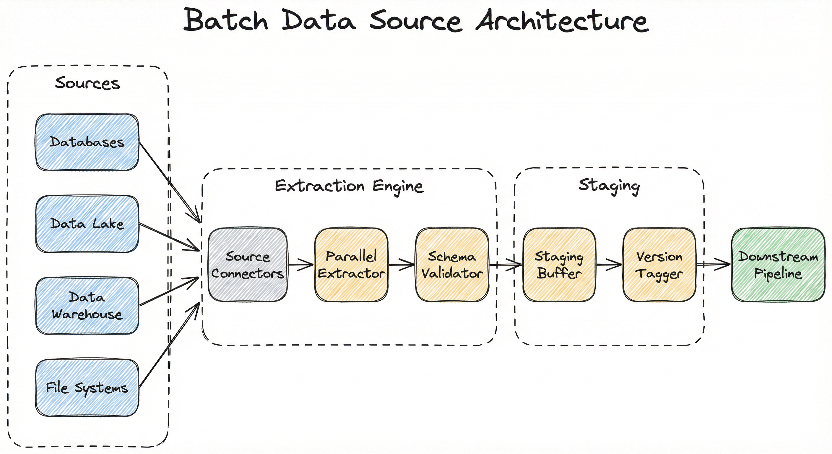
A production batch data source system is built around four key subsystems: source connectors that interface with diverse data stores, an extraction engine that handles parallel reads and predicate pushdown, a staging layer that buffers extracted data before handoff, and a versioning and metadata layer that tracks lineage and enables reproducibility.
The architecture must handle heterogeneous sources -- a single ML pipeline might pull user profiles from PostgreSQL, clickstream logs from S3 Parquet files, and product catalogs from a data warehouse -- all within one extraction job.
The extraction engine is where most of the engineering complexity lives. It must handle connection pooling for databases, parallel file listing for object storage, partition pruning for data lake tables, and format-specific deserialization for different file types. At scale, this is typically implemented on Apache Spark, Dask, or Ray, with the source connectors acting as thin adapters over the distributed read framework.
Key Components
Source Connectors
Adapters that interface with specific data stores -- JDBC/ODBC for relational databases, S3/GCS/ADLS clients for object storage, HDFS readers for Hadoop clusters, and file parsers for local or network-attached storage. Each connector handles authentication, connection pooling, and source-specific query optimization (e.g., predicate pushdown to the database engine).
Parallel Extraction Engine
Distributes the read workload across multiple workers. For database sources, this means splitting the query by key ranges or partitions. For file-based sources, it means listing and assigning files or file chunks to workers in parallel. Spark's DataFrameReader, Dask's read_parquet(), and Ray Data's read_datasource() all implement this pattern.
Schema Validator
Validates that the extracted data conforms to the expected schema -- column names, data types, nullability constraints. Catches upstream schema changes (column renames, type changes, dropped columns) before they propagate to training pipelines and cause silent model degradation.
Staging Buffer
Temporarily holds extracted data in a landing zone (often an S3 bucket or local disk) before it moves into the pipeline. This decouples extraction from downstream processing, enabling retries without re-reading the source and providing a checkpoint for recovery.
Version Tagger / Metadata Layer
Tags each extraction batch with metadata: timestamp, source query/path, schema version, row counts, checksums. Integrates with data versioning tools (DVC, lakeFS, Delta Lake time travel) to enable exact reproduction of any historical extraction.
Incremental State Tracker
Maintains the high-water mark (last extracted timestamp, offset, or snapshot ID) for incremental loading. Persisted in a metadata store so subsequent runs know where to resume. Must be updated atomically with the extraction to prevent data loss or duplication.
Data Flow
Full Extraction Path: The extraction engine connects to the source via the appropriate connector -> issues a full read (optionally with partition filters) -> data streams through the schema validator -> lands in the staging buffer -> gets tagged with version metadata -> is handed off to the downstream pipeline.
Incremental Extraction Path: The state tracker retrieves the last high-water mark -> the extraction engine reads only records newer than the mark -> schema validation and staging proceed as above -> the state tracker updates the high-water mark atomically upon successful completion.
Multi-Source Extraction: When a pipeline needs data from multiple sources, the extraction engine runs connectors in parallel (or sequentially with dependency ordering). Each source's output lands in the staging buffer independently. A join or merge step downstream combines them. This pattern is common in feature engineering pipelines -- for example, joining user profile data from PostgreSQL with clickstream events from S3.
A directed flow showing four source types (Databases, Data Lake, Data Warehouse, File Systems) feeding into Source Connectors, which pass data through a Parallel Extractor and Schema Validator in the Extraction Engine, then to a Staging Buffer and Version Tagger in the Staging layer, finally outputting to the Downstream Pipeline.
How to Implement
Two Implementation Paradigms
Batch data source implementations fall into two categories based on scale:
Paradigm 1: Single-machine loading using Pandas, Polars, or DuckDB. Suitable for datasets that fit in memory (up to ~50-100 GB on modern machines with memory-mapped files). This is where most data scientists start, and it's perfectly adequate for many use cases. A startup in Bengaluru training a fraud detection model on 10M transaction records (about 5 GB) doesn't need Spark.
Paradigm 2: Distributed loading using Apache Spark, Dask, Ray Data, or cloud-native services (AWS Glue, Azure Data Factory, GCP Dataflow). Required when data exceeds single-machine capacity or when you need parallelized extraction from partitioned sources. Flipkart processing 10+ TB daily or Netflix reading from their petabyte-scale Iceberg data lake -- these require distributed extraction.
The choice is driven by data volume, latency requirements, and team expertise. A common anti-pattern is reaching for Spark when Pandas would suffice -- the overhead of cluster management, serialization, and job scheduling adds weeks of engineering effort for no benefit at small scale.
Cost Comparison: A single
r6i.4xlargeinstance on AWS (128 GB RAM) costs about 3.03/hour (~INR 254/hour) plus EMR overhead of $0.27/hour. For datasets under 50 GB, the single-machine approach saves ~65% on compute costs.
File Format Selection
The choice of file format dramatically impacts read performance:
| Format | Type | Compression | Predicate Pushdown | Column Pruning | Best For |
|---|---|---|---|---|---|
| Parquet | Columnar | Snappy, Zstd, Gzip | Yes | Yes | Analytical/ML workloads |
| ORC | Columnar | Zlib, Snappy | Yes | Yes | Hive-heavy ecosystems |
| Avro | Row-based | Deflate, Snappy | No | No | Schema evolution, streaming |
| CSV | Row-based | None (external) | No | No | Human-readable, small data |
| JSON/JSONL | Row-based | None (external) | No | No | Semi-structured, APIs |
| TFRecord | Row-based | Gzip | No | No | TensorFlow training |
For ML workloads, Parquet is the default choice. Its columnar layout means that if your model only uses 20 out of 200 columns, you read 10x less data. Combined with predicate pushdown, a well-partitioned Parquet dataset can reduce I/O by 50-100x compared to reading raw CSV.
import pandas as pd
import pyarrow.parquet as pq

# Read only specific columns and partitions from a partitioned Parquet dataset
# Dataset partitioned by date: s3://data-lake/events/date=2025-01-01/
dataset = pq.ParquetDataset(
    "s3://data-lake/events/",
    filters=[("date", ">=", "2025-01-01"), ("date", "<", "2025-02-01")],
    use_legacy_dataset=False,
)

# Read only the columns needed for feature engineering
df = dataset.read(
    columns=["user_id", "event_type", "timestamp", "amount", "category"],
).to_pandas()

print(f"Loaded {len(df):,} rows, {df.memory_usage(deep=True).sum() / 1e6:.1f} MB")

# Validate schema expectations
expected_columns = {"user_id", "event_type", "timestamp", "amount", "category"}
assert set(df.columns) == expected_columns, f"Schema mismatch: {set(df.columns) - expected_columns}"
assert df["amount"].dtype == "float64", "Amount column type changed!"

# Tag this extraction for reproducibility
extraction_metadata = {
    "source": "s3://data-lake/events/",
    "date_range": "2025-01-01 to 2025-01-31",
    "row_count": len(df),
    "columns": list(df.columns),
    "checksum": pd.util.hash_pandas_object(df).sum(),
}
This example demonstrates the single-machine approach using PyArrow's ParquetDataset for partition-pruned reads from S3. The key patterns are: (1) partition filtering to avoid reading months of data when you need one month, (2) column projection to read only the features you need, (3) schema validation to catch upstream changes, and (4) extraction metadata for reproducibility. For a 100 GB dataset with 200 columns where you need 5 columns and 1 month of 12, this reads ~4 GB instead of 100 GB.
from pyspark.sql import SparkSession
from pyspark.sql import functions as F
from datetime import datetime
import json

spark = SparkSession.builder \
    .appName("batch-data-source") \
    .config("spark.sql.sources.partitionOverwriteMode", "dynamic") \
    .config("spark.sql.parquet.mergeSchema", "true") \
    .getOrCreate()

# --- Incremental Loading with High-Water Mark ---
def get_high_water_mark(state_path: str) -> str:
    """Retrieve the last successful extraction timestamp."""
    try:
        state = spark.read.json(state_path).first()
        return state["high_water_mark"]
    except Exception:
        return "1970-01-01T00:00:00"  # First run: extract everything

def update_high_water_mark(state_path: str, new_mark: str):
    """Atomically update the high-water mark after successful extraction."""
    state_df = spark.createDataFrame(
        [{"high_water_mark": new_mark, "updated_at": datetime.utcnow().isoformat()}]
    )
    state_df.coalesce(1).write.mode("overwrite").json(state_path)

# Read the high-water mark
state_path = "s3://ml-pipeline/state/events_hwm/"
hwm = get_high_water_mark(state_path)

# Incremental extraction: read only new records
df = spark.read.parquet("s3://data-lake/events/") \
    .filter(F.col("updated_at") > hwm) \
    .select("user_id", "event_type", "timestamp", "amount", "category")

# Schema validation
expected_schema = ["user_id", "event_type", "timestamp", "amount", "category"]
assert df.columns == expected_schema, f"Schema drift detected: {df.columns}"

# Cache and compute metrics
df.cache()
row_count = df.count()
max_ts = df.agg(F.max("updated_at")).first()[0]

print(f"Extracted {row_count:,} incremental rows since {hwm}")

# Write to staging area in optimized format
df.write \
    .mode("append") \
    .partitionBy("event_type") \
    .parquet("s3://ml-pipeline/staging/events/")

# Update high-water mark only after successful write
if row_count > 0:
    update_high_water_mark(state_path, max_ts)
This PySpark example demonstrates incremental loading -- the most important optimization for batch data sources at scale. Instead of re-reading the entire dataset on every pipeline run, it tracks a high-water mark (the timestamp of the last extracted record) and reads only the delta. For a table growing at 1% per day, this reduces daily extraction volume by 99%. The pattern also includes schema validation, staging writes with partitioning, and atomic high-water mark updates. Note the mergeSchema config -- essential for handling schema evolution in Parquet datasets.
import pandas as pd
from sqlalchemy import create_engine, text
from contextlib import contextmanager
from typing import Iterator

# Connection pooling for production database reads
engine = create_engine(
    "postgresql://reader:[email protected]:5432/analytics",
    pool_size=5,
    max_overflow=10,
    pool_timeout=30,
    pool_recycle=3600,  # Recycle connections every hour
)

@contextmanager
def read_connection():
    """Context manager for safe connection handling."""
    conn = engine.connect()
    try:
        yield conn
    finally:
        conn.close()

def extract_in_chunks(
    query: str,
    chunk_size: int = 50_000,
    params: dict = None,
) -> Iterator[pd.DataFrame]:
    """Extract data in memory-efficient chunks.

    Critical: Always read from a READ REPLICA, never from
    the primary database serving production traffic.
    """
    with read_connection() as conn:
        for chunk in pd.read_sql(
            text(query),
            conn,
            chunksize=chunk_size,
            params=params,
        ):
            # Validate each chunk's schema
            yield chunk

# Usage: extract user features for ML training
query = """
    SELECT user_id, signup_date, total_orders, avg_order_value,
           last_active_at, city, is_premium
    FROM user_features
    WHERE last_active_at >= :start_date
      AND last_active_at < :end_date
    ORDER BY user_id
"""

chunks = []
for chunk in extract_in_chunks(
    query,
    chunk_size=100_000,
    params={"start_date": "2025-01-01", "end_date": "2025-02-01"},
):
    chunks.append(chunk)
    print(f"  Extracted chunk: {len(chunk):,} rows")

df = pd.concat(chunks, ignore_index=True)
print(f"Total extracted: {len(df):,} rows")

# Save to Parquet for downstream pipeline
df.to_parquet("staging/user_features_202501.parquet", index=False)
This example shows the critical pattern of reading from a database for ML training -- something almost every team does but often gets wrong. Key practices: (1) Always use a read replica, never the primary database. A full table scan on a production database serving Razorpay's payment API would be catastrophic. (2) Chunked reads to handle datasets larger than memory. (3) Connection pooling to reuse connections efficiently. (4) Parameterized queries to prevent SQL injection and enable incremental extraction. (5) Convert to Parquet immediately -- you never want downstream pipeline stages re-querying the database.
# dvc.yaml - Pipeline definition with versioned data
# stages:
#   extract:
#     cmd: python extract_training_data.py
#     deps:
#       - extract_training_data.py
#     params:
#       - extract.start_date
#       - extract.end_date
#       - extract.source_table
#     outs:
#       - data/training/raw/

# extract_training_data.py
import yaml
import pandas as pd
from pathlib import Path

# Load parameters from params.yaml (tracked by DVC)
with open("params.yaml") as f:
    params = yaml.safe_load(f)["extract"]

print(f"Extracting from {params['source_table']}")
print(f"Date range: {params['start_date']} to {params['end_date']}")

# Extract data (using any connector -- DB, S3, etc.)
df = pd.read_parquet(
    f"s3://data-lake/{params['source_table']}/",
    filters=[
        ("date", ">=", params["start_date"]),
        ("date", "<", params["end_date"]),
    ],
)

# Save locally -- DVC will track and version this output
output_path = Path("data/training/raw/")
output_path.mkdir(parents=True, exist_ok=True)
df.to_parquet(output_path / "training_data.parquet", index=False)

# Print metrics for DVC tracking
print(f"Rows extracted: {len(df):,}")
print(f"Columns: {list(df.columns)}")
print(f"Size: {(output_path / 'training_data.parquet').stat().st_size / 1e6:.1f} MB")

# --- CLI Usage ---
# dvc init
# dvc run -n extract -d extract_training_data.py \
#         -p extract.start_date,extract.end_date,extract.source_table \
#         -o data/training/raw/ \
#         python extract_training_data.py
#
# dvc push  # Push data to remote storage (S3, GCS, Azure)
# git add dvc.yaml dvc.lock params.yaml
# git commit -m "Extract training data for Jan 2025"
#
# To reproduce later:
# git checkout <commit-hash>
# dvc pull
# dvc repro
This example demonstrates data versioning with DVC -- essential for ML reproducibility. DVC tracks large data files alongside your Git history without storing them in Git. The key insight is that dvc.lock records the exact MD5 hash of your extracted data, so months later you can git checkout + dvc pull to recover the exact training dataset that produced a given model. The params.yaml file parameterizes the extraction so you can easily change date ranges or source tables. This pattern is used extensively in Indian ML teams at companies like Ola, PhonePe, and Jio where regulatory compliance requires data lineage tracking.
from pyspark.sql import SparkSession
from delta.tables import DeltaTable

spark = SparkSession.builder \
    .appName("delta-batch-read") \
    .config("spark.jars.packages", "io.delta:delta-spark_2.12:3.1.0") \
    .config("spark.sql.extensions", "io.delta.sql.DeltaSparkSessionExtension") \
    .config("spark.sql.catalog.spark_catalog", "org.apache.spark.sql.delta.catalog.DeltaCatalog") \
    .getOrCreate()

# Read the latest version of a Delta table
df_latest = spark.read.format("delta").load("s3://data-lake/transactions/")

# Time travel: read the table as it existed at a specific version
df_v42 = spark.read.format("delta") \
    .option("versionAsOf", 42) \
    .load("s3://data-lake/transactions/")

# Time travel: read the table as of a specific timestamp
df_jan = spark.read.format("delta") \
    .option("timestampAsOf", "2025-01-15T00:00:00Z") \
    .load("s3://data-lake/transactions/")

# Schema evolution: the table may have added columns over time
# Delta Lake handles this transparently -- new columns appear as NULL
# for older records
print(f"Current schema: {df_latest.schema.fieldNames()}")
print(f"V42 schema:     {df_v42.schema.fieldNames()}")

# Read incremental changes between versions (Change Data Feed)
changes = spark.read.format("delta") \
    .option("readChangeFeed", "true") \
    .option("startingVersion", 40) \
    .option("endingVersion", 42) \
    .load("s3://data-lake/transactions/")

# Filter to only new inserts (skip updates and deletes)
new_records = changes.filter(changes["_change_type"] == "insert")
print(f"New records between v40 and v42: {new_records.count():,}")
Delta Lake adds ACID transactions, schema evolution, and time travel to Parquet-based data lakes. This is critical for ML batch sources because: (1) Time travel lets you reproduce training data from any historical point without maintaining separate snapshots. (2) Schema evolution handles upstream changes gracefully -- if the data team adds a new column, your pipeline doesn't break. (3) Change Data Feed enables efficient incremental extraction by reading only the changes between versions rather than re-scanning the entire table. This pattern is widely used on Databricks, where many Indian enterprises (HDFC Bank, Reliance, Tata Group) run their ML data infrastructure.
# batch_source_config.yaml
source:
  type: parquet
  path: s3://data-lake/events/
  format_options:
    merge_schema: true
    predicate_pushdown: true

extraction:
  mode: incremental  # or 'full'
  incremental_key: updated_at
  state_store: s3://ml-pipeline/state/events/
  partition_filter:
    date: ">=2025-01-01"
    region: ["IN", "US", "EU"]

schema:
  validation: strict  # strict | warn | skip
  expected_columns:
    - name: user_id
      type: string
      nullable: false
    - name: amount
      type: float64
      nullable: true
    - name: event_type
      type: string
      nullable: false

output:
  format: parquet
  compression: snappy
  staging_path: s3://ml-pipeline/staging/events/
  partition_by: [event_type, date]

versioning:
  enabled: true
  tool: dvc  # or 'lakefs', 'delta'
  tag_template: "events-{date}-{run_id}"

retry:
  max_attempts: 3
  backoff_seconds: [10, 60, 300]
  idempotent: true
Common Implementation Mistakes
- ●
Reading from the primary database: Running full-table-scan extraction queries against a production database instead of a read replica. This can spike database CPU to 100%, increase latency for production queries, and potentially cause an outage. Always set up a dedicated read replica for ML batch extractions.
- ●
Ignoring schema evolution: Hard-coding column names and types without validation. When the upstream data team renames a column or changes a type (e.g.,
amountfromINTtoDECIMAL), the pipeline silently produces wrong features. Always validate schema on read. - ●
Full extraction when incremental suffices: Re-reading the entire dataset on every pipeline run instead of tracking a high-water mark and extracting only new records. For a 1 TB table growing at 1% daily, this wastes 99% of I/O and compute every single day.
- ●
Not versioning training data: Training a model on Monday, finding a bug on Friday, and having no way to reproduce Monday's exact training set. Data versioning (DVC, lakeFS, Delta time travel) is not optional for production ML -- it's a hard requirement.
- ●
Using CSV for large datasets: CSV is human-readable but catastrophically inefficient for ML workloads -- no column pruning, no compression, no schema enforcement, and ambiguous type inference. Switch to Parquet or ORC for anything beyond exploratory analysis.
- ●
Ignoring data skew in parallel reads: Partitioning a database extraction by a skewed column (e.g.,
citywhere Mumbai has 40% of records) leads to some workers finishing in seconds while one worker takes 10x longer. Use uniform partitioning strategies (hash-based or range-based on a monotonic key). - ●
Missing idempotency: If a batch extraction fails halfway and restarts, does it produce duplicates? Without idempotent writes (upserts or deduplication), you'll silently double-count records in your training data.
When Should You Use This?
Use When
You need to train or retrain an ML model on historical data that doesn't need to be real-time (data can be hours or days old)
The training dataset exceeds what can be loaded from an API or stream in a reasonable time -- batch extraction from a data lake or warehouse is the efficient path
Regulatory or compliance requirements demand that you can reproduce the exact dataset used for any historical model training run (common in Indian fintech under RBI guidelines)
Your data source supports efficient bulk reads (partitioned Parquet on S3, database read replicas, data warehouse exports) but not efficient streaming
Feature engineering requires joining multiple large tables or aggregating over long time windows (e.g., computing 90-day rolling averages from transaction logs)
You're backfilling a feature store with historical values -- this is inherently a batch operation regardless of whether the feature store itself serves in real-time
Data arrives in natural batches (daily files from a partner, weekly data dumps, monthly regulatory reports from SEBI or RBI)
Avoid When
Your ML system requires features computed from events that occurred less than 5 minutes ago -- use a streaming data source instead
The source data is inherently event-driven (user clicks, sensor readings, stock ticks) and you need continuous processing -- batch adds unnecessary latency
Your dataset is small enough to load from a REST API or in-memory cache in seconds -- the overhead of a batch infrastructure is unjustified
The data source provides a change data capture (CDC) stream natively and your pipeline can consume it -- streaming CDC is more efficient than periodic batch polling
You need to react to individual records as they arrive (fraud detection, real-time recommendations) rather than processing them in aggregate
The data is already available in a feature store or pre-materialized view and doesn't need re-extraction
Key Tradeoffs
Latency vs. Cost: The Fundamental Tradeoff
Batch processing trades latency for cost efficiency. A batch job running once daily on a 50-node Spark cluster for 2 hours costs a fraction of what a 24/7 streaming pipeline (Kafka + Flink) would cost for the same data volume. For an Indian startup processing 100 GB/day:
| Approach | Monthly Compute Cost | Data Freshness |
|---|---|---|
| Daily batch (Spark on EMR) | ~$180 (~INR 15,000) | 24 hours |
| Hourly micro-batch | ~$450 (~INR 37,800) | 1 hour |
| Real-time streaming (Kafka + Flink) | ~$1,200 (~INR 1,00,800) | < 1 minute |
For most ML training workloads, 24-hour-old data is perfectly acceptable. Recommendation models, churn predictors, and demand forecasters don't need minute-level freshness for their training data. Save the real-time budget for serving-time features.
Simplicity vs. Completeness
Full extraction is simpler to implement (no state management) but wasteful at scale. Incremental loading is efficient but adds complexity: you need high-water mark tracking, idempotent writes, and handling of late-arriving data. The right choice depends on your data volume and pipeline maturity:
- < 10 GB: Full extraction every run. Don't overthink it.
- 10 GB - 1 TB: Incremental loading with timestamp-based high-water marks.
- > 1 TB: Incremental loading with partition-based extraction or CDC. Consider Delta Lake / Iceberg for built-in change tracking.
Format Flexibility vs. Performance
Supporting every input format (CSV, JSON, Parquet, Avro, ORC, Excel) makes your batch source maximally flexible but slows development and increases maintenance. In practice, standardize on Parquet for analytical/ML workloads and support CSV/JSON only as ingest formats that get immediately converted. The 5-10x compression and column pruning benefits of Parquet compound at scale.
Alternatives & Comparisons
A streaming data source processes records continuously as they arrive (via Kafka, Kinesis, or Pub/Sub), while a batch data source reads records in discrete chunks on a schedule. Choose streaming when you need sub-minute data freshness for serving-time features; choose batch when training on historical data where hours-old freshness is acceptable and cost efficiency matters. Many production ML systems use both -- streaming for online features and batch for offline training.
File upload is a user-driven, typically small-scale data ingestion method (uploading a CSV via a web UI). Batch data source is a programmatic, large-scale extraction from enterprise data stores. Use file upload for one-off datasets or user-contributed data; use batch data source for automated, recurring extraction from databases and data lakes.
A data lake is a storage system; a batch data source is a reading pattern. The data lake is where data lives; the batch data source is how you pull data out of it. They are complementary: in most architectures, the batch data source reads from a data lake. Think of the data lake as the library and the batch data source as the checkout counter.
Pros, Cons & Tradeoffs
Advantages
Cost-efficient at scale: Batch processing amortizes infrastructure costs over large data volumes. Processing 1 TB in a single 2-hour Spark job is 5-10x cheaper than maintaining a 24/7 streaming pipeline for the same throughput.
Simpler error handling and recovery: If a batch job fails, you restart it. The data hasn't gone anywhere. Streaming failures require dealing with offsets, replayability, and ordering guarantees -- significantly more complex.
Natural fit for ML training: Model training is inherently a batch operation -- you need a complete dataset, not a stream. Batch extraction aligns perfectly with the training lifecycle.
Enables data versioning and reproducibility: Discrete batch extractions can be tagged, versioned, and stored as immutable snapshots. This is much harder with continuous streams where the "dataset" is always changing.
Supports complex join and aggregation patterns: Batch processing frameworks (Spark, Dask) excel at multi-table joins, window functions, and aggregations that are awkward or impossible in streaming contexts.
Predictable resource usage: Batch jobs have defined start and end times, making capacity planning straightforward. You know exactly how many compute hours you'll consume per day.
Leverage existing data warehouse investments: Most enterprises already have data warehouses (Snowflake, BigQuery, Redshift) optimized for batch reads. Your batch source can tap into these without additional infrastructure.
Disadvantages
Data freshness is inherently limited: Even with hourly batch runs, your training data is at least an hour old. For domains where data distribution shifts rapidly (stock markets, trending topics), this can degrade model quality.
Large batch jobs can be brittle: A 4-hour Spark job that fails at hour 3 due to a bad record or OOM error wastes significant compute. Checkpointing helps but adds complexity.
Scaling is step-function, not linear: You either run a bigger cluster or you don't. Unlike streaming which can auto-scale with load, batch jobs require upfront capacity planning.
Operational toil for scheduling and monitoring: Someone needs to manage the cron jobs, Airflow DAGs, or orchestrator configs. Failures at 3 AM need alerting and on-call response.
Cold start problem for new pipelines: The first full extraction of a multi-terabyte dataset can take hours or days. Subsequent incremental loads are fast, but the initial backfill is painful.
Schema drift is harder to detect: In streaming, a bad record surfaces immediately. In batch, a schema change might not be noticed until the next daily run processes the affected partition, leading to delayed detection.
Failure Modes & Debugging
Schema Drift Breaking Downstream Pipelines
Cause
Upstream data team renames a column (user_id to customer_id), changes a type (amount from INT to STRING), or drops a column without notifying the ML team. This happens more often than you'd think -- especially in large organizations where data producers and ML consumers are in different teams.
Symptoms
Pipeline crashes with a KeyError or TypeError. In worse cases (type widening like INT to FLOAT), the pipeline succeeds but produces numerically wrong features. Models trained on these features degrade silently.
Mitigation
Implement schema contracts between producers and consumers. Validate schema on every read against an expected specification (see the config example above). Use tools like Great Expectations or Pandera for programmatic schema validation. Subscribe to schema registry change notifications if available. For data lakes, use Delta Lake or Iceberg which enforce schema on write.
Incremental Loading Data Loss
Cause
The high-water mark is updated before the extraction completes successfully, or the high-water mark column has records with NULL timestamps that are never picked up. Alternatively, late-arriving records with timestamps before the current high-water mark are missed.
Symptoms
Row counts gradually decrease compared to full extractions. A reconciliation check shows missing records. Models retrained on incomplete data show unexpected performance degradation, especially for underrepresented cohorts.
Mitigation
Update the high-water mark only after the extraction is fully committed to the staging layer (never before). Handle NULLs in the incremental key explicitly. For late-arriving data, use a lookback window (e.g., re-extract the last 3 days on each run to catch late arrivals). Implement daily reconciliation: compare incremental row counts against a full-count query on the source.
Source Database Overload
Cause
The batch extraction job runs a heavy query (full table scan, expensive joins) against the production database rather than a read replica, or runs during peak hours when the replica is already under load.
Symptoms
Database CPU spikes, query latency for production traffic increases, connection pool exhaustion. In severe cases, the database becomes unresponsive and causes user-facing outages. This is especially dangerous for Indian payment systems (Razorpay, PhonePe) where transaction latency SLAs are strict.
Mitigation
Always extract from a dedicated read replica, not the primary. Schedule batch jobs during off-peak hours. Implement rate limiting or query throttling. For large tables, use chunked reads with LIMIT/OFFSET or partition-based extraction rather than a single monolithic query. Monitor replica lag and pause extraction if lag exceeds thresholds.
Data Skew Causing Worker Straggler
Cause
Parallel extraction is partitioned by a skewed column (e.g., city where Mumbai has 40% of records, or event_type where one type dominates). One worker processes disproportionately more data than others.
Symptoms
Overall job runtime is bottlenecked by one or two slow tasks while other workers sit idle. Spark UI shows massive skew in task durations. Resource utilization is poor -- you're paying for a 50-node cluster but only 2 nodes are doing real work.
Mitigation
Partition by a high-cardinality, uniformly distributed key (e.g., hash(user_id) % num_partitions). If using database extraction, split by primary key ranges rather than categorical columns. In Spark, use repartition() after the initial read to rebalance, or enable adaptive query execution (AQE) which handles skew automatically in Spark 3.x.
Silent Encoding or Type Corruption
Cause
CSV files with inconsistent encoding (UTF-8 vs. Latin-1), or Parquet files written with incompatible type promotions. Common when data comes from multiple sources or legacy systems -- for instance, partner data feeds in Indian retail often use non-standard encodings for addresses containing Hindi/Devanagari characters.
Symptoms
Special characters appear as garbled text or question marks. Numeric columns contain unexpected NaN values from failed type coercion. String columns have invisible control characters that break downstream string operations.
Mitigation
Always specify encoding explicitly when reading CSV (encoding='utf-8'). Use Parquet or Avro for internal data transfer (they embed encoding information). Run a data profiling step after extraction to detect unexpected NULL rates, character distributions, or type anomalies. Tools like ydata-profiling (formerly pandas-profiling) can automate this.
Version Mismatch Between Training and Serving Data
Cause
The batch source for training reads from one version of a table (e.g., with old feature definitions), while the serving-time feature computation uses a different schema or transformation logic. This is the classic training-serving skew introduced at the data source level.
Symptoms
Model performance in production is significantly different from offline evaluation metrics. Feature distributions at serving time don't match training distributions. This is one of the most common and hardest-to-debug issues in production ML.
Mitigation
Use a feature store (Feast, Tecton, Databricks Feature Store) that unifies offline batch extraction and online serving with the same feature definitions. Tag training datasets with the exact feature computation version. Run distribution comparison checks between training features and serving features regularly.
Placement in an ML System
Where Does It Sit in the ML Pipeline?
The batch data source is the first node in any offline ML pipeline. It sits before everything: data validation, cleaning, transformation, feature engineering, training, and evaluation. Nothing happens until the data is extracted.
In a typical ML training pipeline, the batch source reads historical data from a data lake (S3, ADLS, GCS) or database, passes it through validation and cleaning stages, then into feature engineering and finally model training. The entire pipeline runs on a schedule (daily, weekly) or is triggered by events (new data arrival, model retraining request).
In a feature store backfill scenario, the batch source reads historical data, computes features using the same transformation logic as the online serving path, and writes the results to the offline feature store. This enables training on features that are consistent with what the model will see at serving time.
For evaluation and monitoring, batch sources read production logs and ground-truth labels to compute model performance metrics offline. This is how Netflix evaluates recommendation quality -- by reading batch interaction logs and computing engagement metrics against model predictions.
Key Insight: The batch data source determines the data quality ceiling for your entire ML pipeline. Schema errors, missing records, or stale data introduced at this stage propagate through every downstream component. Invest in validation and monitoring here -- it pays compound dividends.
Pipeline Stage
Data Ingestion
Upstream
- data-lake
- file-upload
Downstream
- data-validation
- data-cleaning
- data-transformation
- streaming-data-source
Scaling Bottlenecks
The primary bottleneck is I/O throughput -- reading large volumes of data from remote storage or databases. For S3-based data lakes, single-stream read throughput is approximately 100 MB/s per connection. Reading 1 TB sequentially takes ~2.8 hours. With 50 parallel streams, it drops to ~3.5 minutes -- but you need 50 workers to achieve this.
For database sources, the bottleneck is often the database itself. Even a read replica has finite CPU, I/O, and connection capacity. A 100M-row table scan on PostgreSQL might take 30 minutes on a well-tuned replica. At 1B rows, you're looking at hours unless you partition the extraction.
Network bandwidth becomes the constraint at extreme scale. Transferring 10 TB across regions (e.g., from a Mumbai data center to a Spark cluster in AWS ap-south-1) at 1 Gbps takes ~22 hours. Data locality -- running compute where the data lives -- is the only real solution.
For Spark-based extraction, the driver node can become a bottleneck if it collects too much metadata or handles excessive shuffle coordination. Keep the driver lightweight; push all data processing to executors.
Production Case Studies
Uber's Michelangelo platform uses batch data pipelines extensively for offline feature engineering and model training. Their workflow engine Piper orchestrates batch extraction from HDFS and Hive data warehouses, computing features like "average trip time in the last 30 days" and "driver rating percentile" through Spark jobs. The batch pipeline handles hundreds of ML models across pricing, ETA prediction, fraud detection, and driver matching.
Michelangelo's batch pipeline reduced the time from model ideation to production deployment from months to weeks. The platform supports thousands of batch feature computation jobs daily, processing petabytes of data for offline model training across Uber's global operations.
Netflix's ML infrastructure reads batch training data from their S3-based Apache Iceberg data lake using Spark. Their recommendation models, content valuation models, and A/B testing analysis all rely on batch extraction of user interaction logs (views, searches, ratings) and content metadata. The batch pipeline processes several terabytes of interaction data daily, with Spark handling distributed reads and feature computation.
The batch data infrastructure supports diverse ML systems across the company -- from deep learning recommendation models to statistical A/B testing frameworks -- all reading from the same versioned data lake with reproducible extraction patterns.
Zerodha, India's largest retail stockbroker, processes batch profit-and-loss (PnL) calculations for over 3 million customers daily. Their batch pipeline ingests 100+ million transactional records from their trading systems, processes them through containerized AWS Batch jobs with Redis-backed intermediate storage, and produces per-customer PnL reports. The data grows 4x during processing due to derived calculations.
By migrating from sequential processing to parallelized AWS Batch, Zerodha reduced PnL processing time from 7 hours to 20-30 minutes -- a 14-21x speedup -- while maintaining accuracy across 100M+ records and serving results to customers before market open.
Flipkart's data platform processes 10+ TB of raw data daily (50+ TB during Big Billion Days sales), ingesting batch data from multiple sources including transaction logs, product catalogs, and user interaction streams. Their ML models for search ranking, recommendation, and pricing rely on batch feature extraction from their data lake. The platform migrated to Google Cloud, processing 10 PB of batch data and 2 PB of near-real-time data daily.
The batch data infrastructure supports 130+ billion messages per day ingestion and powers ML models serving 400+ million registered users, with the platform processing 60 TB of compressed data daily during regular operations.
LinkedIn's Venice platform serves as a derived data store that ingests batch-processed outputs from Spark and Hadoop jobs. For ML features, batch pipelines compute features like "profile view counts in the last 7 days" and "connection graph metrics" that are then loaded into Venice for online serving via their feature store Feathr. The batch extraction handles petabytes of member interaction data across 900+ million profiles.
Venice powers 1800+ derived datasets used by 300+ distinct applications, including LinkedIn's core recommendation and search ML models, all fed by batch data pipelines running on Spark.
Tooling & Ecosystem
The de facto standard for distributed batch data processing. Spark's DataFrameReader supports Parquet, ORC, CSV, JSON, JDBC, Delta Lake, Iceberg, and Hudi sources. Handles terabyte-scale extraction with partition pruning, predicate pushdown, and columnar read optimization. Used by Netflix, Uber, Flipkart, and virtually every large-scale ML platform.
Column-oriented file format optimized for analytical and ML workloads. Provides 2-10x compression over CSV, supports predicate pushdown and column pruning, and is the default storage format for Spark, Pandas, and most data lake architectures. Essential for efficient batch data reads.
Open-source tool for versioning datasets and ML pipelines. Tracks large files via content-addressable storage while keeping version metadata in Git. Enables exact reproduction of any historical training dataset. Supports S3, GCS, Azure, and SSH remotes.
Git-like version control for data lakes. Provides branching, committing, and merging for datasets stored on S3, GCS, or Azure Blob Storage. Enables atomic versioning of entire data lake partitions, making it ideal for reproducible batch extraction in ML pipelines.
Open-source lakehouse storage layer that adds ACID transactions, schema enforcement, time travel, and change data feed to Parquet-based data lakes. Enables versioned, schema-evolving batch reads. The backbone of Databricks' lakehouse platform used by HDFC Bank, Reliance, and many Indian enterprises.
Open table format for large analytical datasets. Supports schema evolution, hidden partitioning, time travel, and snapshot isolation. Used by Netflix for their production data lake. Enables efficient incremental batch reads via snapshot-based change tracking.
The standard single-machine data manipulation library for Python. pd.read_parquet(), pd.read_sql(), and pd.read_csv() are the most common batch data loading functions in ML notebooks and small-scale pipelines. Suitable for datasets up to ~10-50 GB.
High-performance DataFrame library written in Rust with Python bindings. 5-10x faster than Pandas for many operations due to lazy evaluation, query optimization, and multi-threaded execution. Excellent for batch loading datasets in the 1-100 GB range on a single machine.
In-process analytical database that can directly query Parquet, CSV, and JSON files (including on S3) without loading them into memory. Perfect for batch data exploration and extraction when you need SQL semantics over file-based data lakes.
Workflow orchestrator for scheduling and monitoring batch data pipelines. While not a data source itself, Airflow orchestrates the extraction -- triggering Spark jobs, managing dependencies, and handling retries. Used by nearly every production ML team for batch pipeline scheduling.
Data validation framework that integrates with batch extraction pipelines. Defines "expectations" (schema, value ranges, uniqueness) that are validated on every batch read. Essential for catching data quality issues before they reach the ML model.
Research & References
Murray, Ananthanarayanan, Hung, et al. (2021)VLDB 2021
Describes Google's tf.data framework for building efficient input pipelines for ML training. Covers software pipelining, parallel I/O, caching, and transformation fusion -- foundational techniques for batch data loading in TensorFlow-based systems.
Armbrust, Ghodsi, Xin, Zaharia, et al. (2021)CIDR 2021
Introduced the lakehouse paradigm combining data lake flexibility with data warehouse reliability. Proposes Delta Lake as the storage layer that unifies batch ETL, streaming, and ML workloads on a single data platform.
Koutsoukos, Chrysogelos, Sanca, Ailamaki, et al. (2024)arXiv preprint
Proposes a columnar storage system optimized for ML preprocessing pipelines. Demonstrates that modern batch ML pipelines require extensive preprocessing across multiple models, and that columnar storage with late materialization dramatically reduces I/O for feature extraction.
Jain, Padhye, et al. (2023)CIDR 2023
Comprehensive comparison of Delta Lake, Apache Iceberg, and Apache Hudi -- the three dominant lakehouse formats. Analyzes their approaches to schema evolution, time travel, and incremental reads that are critical for ML batch data sources.
Zhao, Jain, Ramanathan, et al. (2023)arXiv preprint
Applies reinforcement learning to automatically optimize data pipeline configurations (prefetch sizes, parallelism, caching) for training deep recommendation models. Demonstrates that data pipeline tuning can yield 2-3x training throughput improvements.
Databricks Engineering (2019)Databricks Blog (Technical Reference)
Describes the Bronze-Silver-Gold data quality pattern for ML pipelines using Delta Lake. Bronze tables hold raw batch-ingested data, Silver tables contain cleaned and validated data, and Gold tables are ML-ready feature datasets.
Interview & Evaluation Perspective
Common Interview Questions
- ●
How would you design a batch data ingestion pipeline for training a recommendation model on 500 million user interaction logs?
- ●
What is the difference between full extraction and incremental loading? When would you choose each?
- ●
How do you handle schema evolution when the upstream data source adds or removes columns?
- ●
Explain how you would ensure reproducibility of training data across model retraining cycles.
- ●
Why is reading from a production database directly for ML training a bad idea? What's the alternative?
- ●
How would you partition a large batch extraction to parallelize reads efficiently?
- ●
What file format would you choose for storing ML training data and why?
Key Points to Mention
- ●
Always extract from read replicas, never from production databases. This is non-negotiable for systems serving live traffic -- especially payment systems (Razorpay, PhonePe) or trading platforms (Zerodha) where latency spikes have direct business impact.
- ●
Incremental loading with high-water mark tracking reduces extraction volume by 90-99% for append-heavy tables. The high-water mark must be updated after successful write to the staging layer, never before.
- ●
Parquet is the default format for ML batch data. Column pruning + predicate pushdown + compression yield 10-100x I/O reduction compared to CSV. Mention specific numbers: 2-10x compression, 5-50x speedup from column pruning.
- ●
Data versioning (DVC, lakeFS, Delta time travel) is mandatory for production ML. You must be able to answer: 'What exact data produced model v47?' Regulatory requirements in Indian fintech (RBI guidelines) make this a compliance issue, not just a nice-to-have.
- ●
Schema validation on every read catches upstream drift before it reaches model training. A column rename or type change should trigger a pipeline failure, not silent feature corruption.
- ●
Mention the Bronze-Silver-Gold pattern: raw ingested data (Bronze) -> cleaned and validated (Silver) -> ML-ready features (Gold). This is the standard architecture for lakehouse-based ML pipelines.
Pitfalls to Avoid
- ●
Saying 'just use Spark for everything' without discussing scale thresholds. For datasets under 50 GB, Pandas/Polars/DuckDB on a single machine is simpler, faster to develop, and cheaper to run. Always justify the tool choice with data volume.
- ●
Ignoring the operational aspects: who schedules the batch job? What happens when it fails at 3 AM? How do you alert? Airflow DAGs, retry policies, and SLA monitoring are part of the design, not afterthoughts.
- ●
Treating batch data loading as a solved problem that doesn't need monitoring. Schema drift, data volume anomalies, and extraction latency all need dashboards and alerts.
- ●
Not discussing idempotency. If the extraction job fails halfway and is restarted, will it produce duplicates? Production systems must handle retries gracefully.
- ●
Forgetting about data skew when discussing parallel extraction. Interviewers want to hear that you've dealt with real-world partitioning challenges, not just textbook parallelism.
Senior-Level Expectation
A senior or staff engineer should discuss the full design: source selection and connection management (replicas, connection pooling, query optimization), extraction strategy (full vs. incremental with quantitative justification), format selection (Parquet with specific compression and encoding choices), schema management (contracts, validation, evolution handling), data versioning (DVC/lakeFS/Delta with lifecycle policies), orchestration (Airflow DAGs with retry and alerting), monitoring (data freshness SLAs, volume anomaly detection, schema drift alerts), and cost optimization (right-sizing compute, spot instances for batch jobs, storage tiering). The ability to design a batch extraction pipeline that is both cost-efficient for an Indian startup (~INR 15,000/month) and robust enough for Flipkart-scale volumes (10+ TB/day) is what distinguishes senior candidates.
Summary
A batch data source is the entry point for historical data into ML pipelines -- reading from databases, data lakes, and file systems in discrete, scheduled chunks. It's the unglamorous but critical first node that determines the data quality ceiling for everything downstream.
The key engineering decisions are: extraction strategy (full vs. incremental, with incremental loading reducing I/O by 90-99% for growing tables), file format (Parquet for columnar efficiency with 10-100x I/O reduction over CSV), schema management (validation on every read with evolution support via Delta Lake/Iceberg), and data versioning (DVC, lakeFS, or lakehouse time travel for reproducibility). At scale, distributed frameworks like Apache Spark handle parallelized extraction from partitioned data lakes, while single-machine tools (Pandas, Polars, DuckDB) serve workloads under ~50 GB efficiently and cheaply.
Production batch data sources at companies like Uber (Michelangelo), Netflix (Iceberg on S3), Flipkart (10+ TB daily), and Zerodha (100M+ transactional records) demonstrate that this component requires serious engineering: connection management, incremental state tracking, schema contracts, idempotent writes, and monitoring for data freshness and volume anomalies. The cost scales from ~INR 3,000/month for a startup processing 50 GB/day to ~INR 4-5 lakh/month for terabyte-scale daily extraction. In every case, the principle is the same: extract reliably, version everything, validate always, and never touch the production database.