Hyperparameter Tuning in Machine Learning
Hyperparameter tuning is the process of systematically searching for the optimal configuration of values that govern a machine learning model's learning process -- values that are set before training begins and cannot be learned from the data itself.
Every ML model has two kinds of knobs: parameters (learned during training, like neural network weights) and hyperparameters (set by the engineer, like learning rate, batch size, number of layers, regularization strength). The distinction matters because hyperparameters define the space in which the model searches for good parameters. Get the hyperparameters wrong, and even a perfect architecture will converge to a mediocre solution.
Why has this become such a critical component of ML systems? Because the performance gap between default hyperparameters and well-tuned ones is often 5-30% in accuracy or loss -- sometimes the difference between a model that ships and one that doesn't. From a startup in Bengaluru fine-tuning a language model on a single A100 to Google training PaLM across thousands of TPUs, hyperparameter tuning is the universal bottleneck that every ML practitioner must confront.
This guide covers everything from classical grid search to modern approaches like Bayesian optimization, Hyperband, and BOHB, along with practical tooling comparisons (Optuna, Ray Tune, W&B Sweeps, SigOpt) and cost analysis relevant to Indian ML teams operating under tight GPU budgets.
Concept Snapshot
- What It Is
- A systematic search over the space of model configuration values (hyperparameters) to find the combination that optimizes a given performance metric on held-out validation data.
- Category
- Model Training
- Complexity
- Intermediate
- Inputs / Outputs
- Inputs: training data, validation data, a model architecture, and a defined search space. Outputs: the best hyperparameter configuration and associated tuning metrics/history.
- System Placement
- Sits between data preparation (train/test split) and the final training loop in a model training pipeline. Often wraps the training loop as an inner function.
- Also Known As
- hyperparameter optimization, HPO, hyperparameter search, model tuning, hyperparameter selection, AutoML tuning
- Typical Users
- ML Engineers, Data Scientists, Research Scientists, MLOps Engineers, Applied Scientists
- Prerequisites
- Model training fundamentals, Train/test/validation splits, Cross-validation, Overfitting and regularization, Basic probability (for Bayesian methods)
- Key Terms
- search spaceobjective functionacquisition functionsurrogate modelearly stoppingsuccessive halvingTPEGaussian processexpected improvementtrialfidelity
Why This Concept Exists
The Curse of Manual Tuning
In the early days of machine learning, hyperparameter selection was a manual, intuition-driven process. Practitioners would train a model, inspect the results, tweak a learning rate or regularization parameter, and retrain. This worked tolerably when models had 2-3 hyperparameters and training took minutes. But modern deep learning models routinely have 10-50+ hyperparameters spanning continuous, discrete, and conditional dimensions -- learning rate, weight decay, dropout rate, number of layers, hidden dimensions, warmup steps, scheduler type, optimizer choice, and dozens more.
Manual tuning at this scale is not just tedious; it's statistically inadequate. Humans are terrible at exploring high-dimensional spaces. We suffer from anchoring bias (sticking near our initial guess), confirmation bias (over-interpreting small improvements), and sequential thinking (testing one parameter at a time when interactions matter).
The Grid Search Era and Its Limitations
The first systematic approach was grid search: define a set of candidate values for each hyperparameter and evaluate every combination. Grid search is exhaustive and reproducible, but it scales catastrophically. With hyperparameters and values each, the search space contains configurations. Even modest settings -- 5 hyperparameters with 10 values each -- require 100,000 evaluations. If each evaluation takes 30 minutes of GPU time, that's 5.7 years of compute.
Bergstra and Bengio's landmark 2012 paper demonstrated that random search finds better configurations than grid search in the same compute budget, precisely because it samples more unique values along each dimension. This was a turning point -- it showed that smarter search strategies could dramatically reduce the cost of hyperparameter tuning.
The Modern Era: From Brute Force to Intelligence
The real breakthrough came with Bayesian optimization (Snoek et al., 2012), which treats hyperparameter tuning as a sequential decision-making problem. Instead of blindly sampling configurations, Bayesian methods build a probabilistic surrogate model of the objective function and use an acquisition function to intelligently decide where to sample next -- balancing exploration (trying uncertain regions) with exploitation (refining promising regions).
More recently, multi-fidelity methods like Hyperband (Li et al., 2018) and BOHB (Falkner et al., 2018) have added another dimension of efficiency: rather than training every configuration to completion, they evaluate many configurations cheaply (on small budgets) and progressively allocate more resources to the most promising ones. This can yield 10-100x speedups over standard Bayesian optimization.
Key Takeaway: Hyperparameter tuning exists because the performance gap between arbitrary and optimal hyperparameters is too large to ignore, the search space is too vast for manual exploration, and modern methods can find near-optimal configurations with a fraction of the compute that brute-force methods require.
Core Intuition & Mental Model
The Mental Model: House Hunting
Think of hyperparameter tuning like searching for an apartment in Mumbai. You have a budget (compute), a set of criteria (validation metric), and a vast space of options (hyperparameter configurations). Here are three approaches:
Grid search is like visiting every apartment in a fixed grid of neighborhoods, price ranges, and sizes. Thorough but absurdly expensive. You'll spend months visiting places that are obviously wrong.
Random search is like asking a real estate agent to show you random apartments across the city. Surprisingly effective -- you'll stumble onto good neighborhoods faster than the grid approach because you're not wasting time on every permutation in a bad area.
Bayesian optimization is like hiring a brilliant agent who learns your preferences from each visit. After showing you 5 apartments, the agent builds a mental model of what you like, then strategically picks the next apartment to show -- one that's either in a promising area (exploitation) or a completely unexplored neighborhood that might be amazing (exploration). Each visit makes the agent smarter.
What Hyperparameter Tuning Does NOT Do
Let me be clear about the boundaries. Hyperparameter tuning optimizes the configuration of a model, not its architecture. It won't tell you to switch from a CNN to a Transformer, or from XGBoost to a neural network. Those are architecture search / model selection problems (related but distinct).
Hyperparameter tuning also cannot compensate for fundamentally bad data. If your training data is noisy, biased, or insufficient, no amount of learning rate tuning will save you. Fix the data first.
The Core Tradeoff
Every hyperparameter tuning method navigates the same fundamental tension: exploration vs. exploitation. Spend too much time exploring and you waste compute on bad configurations. Spend too much time exploiting and you get stuck in local optima. The art of hyperparameter tuning is managing this tension efficiently.
Expert Note: The single most impactful thing you can do before running any HPO is to reduce your search space using domain knowledge. Don't search learning rates from to when you know your problem class works well between and . A tight, well-informed search space is worth more than a sophisticated search algorithm.
Technical Foundations
Problem Formulation
Hyperparameter optimization can be formally stated as follows. Given a machine learning algorithm with hyperparameter space , a dataset , and a performance metric , find:
where denotes the model trained with hyperparameters on training data , and evaluates the resulting model on .
The function is our objective function. It is typically expensive to evaluate (requires full model training), noisy (due to random initialization and data shuffling), black-box (no gradient available), and potentially non-convex with many local optima.
Random Search
Random search samples configurations independently from the search space: for where is the budget. Bergstra and Bengio (2012) proved that random search is more efficient than grid search when some hyperparameters matter more than others. If only out of hyperparameters are important, grid search wastes of its evaluations exploring irrelevant dimensions, while random search explores distinct values in every dimension.
Bayesian Optimization
Bayesian optimization models with a probabilistic surrogate model -- typically a Gaussian process (GP) -- and uses an acquisition function to select the next configuration to evaluate.
A Gaussian process defines a distribution over functions: where is the mean function and is the covariance (kernel) function. After observing evaluations , the GP posterior provides both a prediction and uncertainty at any unobserved point.
The most common acquisition function is Expected Improvement (EI):
For a GP posterior, this has a closed-form solution:
where , is the standard normal CDF, and is the standard normal PDF.
Tree-structured Parzen Estimator (TPE)
TPE (used by Optuna and Hyperopt) takes a different approach. Instead of modeling directly, it models:
where is a quantile threshold, is the density of good configurations, and is the density of bad ones. The acquisition function becomes:
TPE is more computationally efficient than GP-based methods for high-dimensional and conditional search spaces.
Successive Halving and Hyperband
Hyperband addresses the multi-fidelity aspect of HPO. Instead of training every configuration to completion, it uses successive halving: start configurations with budget , evaluate all, discard the worst half, double the budget for survivors, and repeat.
The total budget for a single bracket of successive halving is:
where is the reduction factor (typically 3). Hyperband runs multiple brackets with different tradeoffs and is theoretically motivated by the infinite-armed bandit framework.
BOHB (Bayesian Optimization + Hyperband)
BOHB combines TPE-guided sampling with Hyperband's multi-fidelity scheduling. Instead of sampling configurations uniformly (as in vanilla Hyperband), BOHB uses a kernel density estimator fitted on the best-performing configurations from completed brackets to guide the search toward promising regions, while still benefiting from early stopping of poor configurations.
Internal Architecture
A hyperparameter tuning system consists of four core subsystems: a search space definition layer that specifies the hyperparameter types and ranges, a search algorithm that proposes candidate configurations, a trial executor that trains and evaluates each configuration, and a result store that persists trial histories for analysis and surrogate model updates.
In distributed settings, an additional scheduler component manages resource allocation across trials -- deciding which trials to continue, pause, or terminate early. This is where multi-fidelity methods like Hyperband operate.
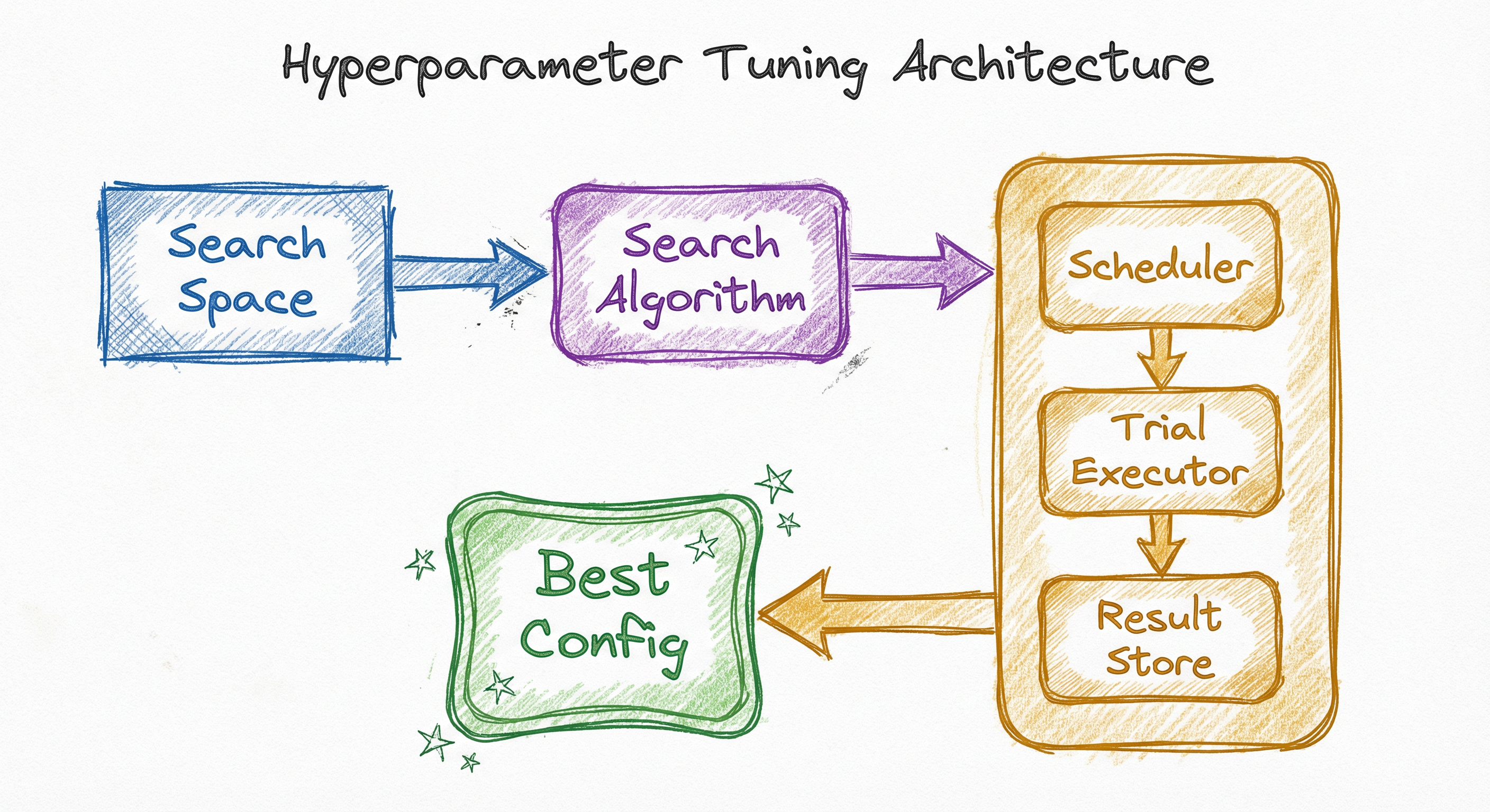
The feedback loop from the result store back to the search algorithm is what makes Bayesian methods powerful -- each completed trial refines the surrogate model, making subsequent suggestions more informed. In contrast, grid and random search have no feedback loop; each trial is independent.
Key Components
Search Space Definition
Declares the hyperparameters to tune, their types (continuous, discrete, categorical, conditional), ranges, and distributions (uniform, log-uniform, etc.). This is the engineer's primary input to the system. A well-defined search space is often more important than the choice of search algorithm.
Search Algorithm (Suggester)
Proposes the next hyperparameter configuration to evaluate. Implements one of: random sampling, grid enumeration, Bayesian optimization (GP or TPE), evolutionary strategies, or population-based methods. Maintains internal state (surrogate model, observation history) that improves over time for model-based methods.
Trial Scheduler
Manages the lifecycle of trials: decides when to start, pause, resume, or terminate a trial. Multi-fidelity schedulers like ASHA (Asynchronous Successive Halving) and Hyperband allocate compute budgets dynamically, killing underperforming trials early and reallocating resources to promising ones.
Trial Executor (Worker Pool)
Runs the actual model training for each configuration. In distributed settings, this is a pool of GPU workers (potentially across multiple machines) that can execute trials in parallel. Each worker receives a configuration, trains the model, reports intermediate and final metrics, and returns results.
Result Store
Persists trial configurations, intermediate metrics (for early stopping), final metrics, and metadata (duration, resource usage). Feeds historical data back to the search algorithm for surrogate model updates. Also serves as the source of truth for post-hoc analysis and visualization.
Checkpoint Manager
Saves and restores model checkpoints for trials that are paused and later resumed (common with Hyperband/ASHA). Handles storage lifecycle to avoid disk exhaustion from accumulating checkpoints of abandoned trials.
Data Flow
Suggest Phase: The search algorithm queries the result store for historical observations, updates its internal model (if model-based), and proposes a new hyperparameter configuration.
Execute Phase: The trial scheduler assigns the configuration to an available worker with an initial resource budget (e.g., 10 epochs). The worker trains the model, reporting intermediate metrics at each checkpoint.
Evaluate Phase: The scheduler monitors intermediate results. For multi-fidelity methods, it compares the trial's performance against peers at the same fidelity level and decides whether to continue (promote to next rung) or terminate (early stop).
Record Phase: Final results (or early-stop results) are written to the result store. The search algorithm is notified and can incorporate the new observation into its surrogate model.
This cycle repeats until the compute budget is exhausted, a target metric is reached, or the search algorithm's improvement rate falls below a threshold.
A directed flow from 'Search Space Definition' -> 'Search Algorithm (TPE/GP/Random)' -> 'Trial Scheduler (Hyperband/ASHA)' -> 'Trial Executor (GPU Workers)' -> 'Result Store (Metrics DB)', with a feedback loop from the Result Store back to the Search Algorithm, and a final output to 'Best Config + Analysis'.
How to Implement
Implementation Approaches
There are three main approaches to implementing hyperparameter tuning, each suited to different scales and team maturities:
Option A: Single-machine library (Optuna, Hyperopt, scikit-learn GridSearchCV) -- runs on one machine, easy to set up, perfect for experiments on a single GPU. An ML engineer in a Bengaluru startup can go from zero to running Bayesian optimization in under 30 minutes.
Option B: Distributed framework (Ray Tune, Optuna with distributed storage) -- scales across a cluster of GPU workers, supports fault tolerance and elastic scaling. Necessary when your tuning budget exceeds what a single machine can handle in a reasonable timeframe.
Option C: Managed service (W&B Sweeps, SigOpt, Google Cloud Vizier, Amazon SageMaker HPO) -- fully managed infrastructure with visualization dashboards and team collaboration features. Best for organizations that want to minimize operational overhead.
Cost Note: A typical hyperparameter tuning run for a medium-sized deep learning model (e.g., fine-tuning a 7B parameter LLM with LoRA) might involve 50-100 trials at 30 minutes each on an A100 GPU. On AWS in Mumbai region, that's roughly 25-50 GPU hours at ~87-175 (~INR 7,300-14,700). With Hyperband, you can often reduce this to 10-15 GPU hours (2/hr), bringing the cost down further to INR 1,700-2,550 for a Hyperband run.
import optuna
from optuna.pruners import HyperbandPruner
import torch
import torch.nn as nn
from torch.utils.data import DataLoader

def objective(trial: optuna.Trial) -> float:
    # Define search space (define-by-run API)
    lr = trial.suggest_float("lr", 1e-5, 1e-2, log=True)
    weight_decay = trial.suggest_float("weight_decay", 1e-6, 1e-2, log=True)
    batch_size = trial.suggest_categorical("batch_size", [16, 32, 64, 128])
    n_layers = trial.suggest_int("n_layers", 2, 6)
    dropout = trial.suggest_float("dropout", 0.1, 0.5)
    optimizer_name = trial.suggest_categorical("optimizer", ["Adam", "AdamW", "SGD"])

    # Build model with suggested hyperparameters
    model = build_model(n_layers=n_layers, dropout=dropout)
    optimizer = getattr(torch.optim, optimizer_name)(
        model.parameters(), lr=lr, weight_decay=weight_decay
    )

    train_loader = DataLoader(train_dataset, batch_size=batch_size, shuffle=True)
    val_loader = DataLoader(val_dataset, batch_size=batch_size)

    # Training loop with intermediate reporting for pruning
    for epoch in range(50):
        train_one_epoch(model, train_loader, optimizer)
        val_loss = evaluate(model, val_loader)

        # Report intermediate value for Hyperband pruning
        trial.report(val_loss, epoch)

        # Prune if this trial is not promising
        if trial.should_prune():
            raise optuna.TrialPruned()

    return val_loss

# Create study with TPE sampler and Hyperband pruner
study = optuna.create_study(
    direction="minimize",
    sampler=optuna.samplers.TPESampler(seed=42),
    pruner=HyperbandPruner(min_resource=3, max_resource=50, reduction_factor=3),
)

study.optimize(objective, n_trials=100, timeout=3600 * 4)  # 4 hour budget

# Results
print(f"Best val_loss: {study.best_value:.4f}")
print(f"Best params: {study.best_params}")

# Visualization
optuna.visualization.plot_optimization_history(study)
optuna.visualization.plot_param_importances(study)
Optuna's define-by-run API lets you construct the search space dynamically inside the objective function, which is powerful for conditional hyperparameters (e.g., only suggest momentum if optimizer is SGD). The HyperbandPruner implements multi-fidelity evaluation -- trials that are clearly underperforming at early epochs are stopped, saving GPU hours. The trial.report() and trial.should_prune() calls enable this communication between the training loop and the scheduler.
from ray import tune
from ray.tune.schedulers import ASHAScheduler
from ray.tune.search.optuna import OptunaSearch
import ray

ray.init(num_gpus=4)  # Use 4 GPUs in parallel

def train_fn(config: dict):
    model = build_model(
        n_layers=config["n_layers"],
        dropout=config["dropout"],
    )
    optimizer = torch.optim.AdamW(
        model.parameters(),
        lr=config["lr"],
        weight_decay=config["weight_decay"],
    )

    for epoch in range(config["max_epochs"]):
        train_loss = train_one_epoch(model, train_loader, optimizer)
        val_loss = evaluate(model, val_loader)

        # Report metrics and save checkpoint
        with tune.checkpoint_dir(epoch) as checkpoint_dir:
            torch.save(model.state_dict(), f"{checkpoint_dir}/model.pt")
        tune.report(val_loss=val_loss, train_loss=train_loss)

search_space = {
    "lr": tune.loguniform(1e-5, 1e-2),
    "weight_decay": tune.loguniform(1e-6, 1e-2),
    "n_layers": tune.randint(2, 7),
    "dropout": tune.uniform(0.1, 0.5),
    "max_epochs": 50,
}

scheduler = ASHAScheduler(
    max_t=50,          # max epochs
    grace_period=5,    # min epochs before pruning
    reduction_factor=3,
)

analysis = tune.run(
    train_fn,
    config=search_space,
    num_samples=100,
    scheduler=scheduler,
    search_alg=OptunaSearch(),  # TPE-guided suggestions
    resources_per_trial={"gpu": 1},
    metric="val_loss",
    mode="min",
    local_dir="~/ray_results",
)

print(f"Best config: {analysis.best_config}")
print(f"Best val_loss: {analysis.best_result['val_loss']:.4f}")
Ray Tune distributes trials across a GPU cluster and combines Optuna's TPE sampler for intelligent configuration proposal with ASHA (Asynchronous Successive Halving) for early stopping. The key advantage over single-machine Optuna is parallelism: with 4 GPUs, you run 4 trials concurrently, potentially reducing wall-clock time by 4x. The resources_per_trial parameter ensures each trial gets exactly one GPU, preventing memory contention.
import wandb

# Define sweep configuration
sweep_config = {
    "method": "bayes",  # Options: grid, random, bayes
    "metric": {"name": "val_loss", "goal": "minimize"},
    "parameters": {
        "learning_rate": {"distribution": "log_uniform_values", "min": 1e-5, "max": 1e-2},
        "weight_decay": {"distribution": "log_uniform_values", "min": 1e-6, "max": 1e-2},
        "batch_size": {"values": [16, 32, 64, 128]},
        "n_layers": {"distribution": "int_uniform", "min": 2, "max": 6},
        "dropout": {"distribution": "uniform", "min": 0.1, "max": 0.5},
        "optimizer": {"values": ["adam", "adamw", "sgd"]},
    },
    "early_terminate": {
        "type": "hyperband",
        "min_iter": 5,
        "eta": 3,
    },
}

def train():
    run = wandb.init()
    config = wandb.config

    model = build_model(n_layers=config.n_layers, dropout=config.dropout)
    optimizer = get_optimizer(model, config.optimizer, config.learning_rate, config.weight_decay)

    for epoch in range(50):
        train_loss = train_one_epoch(model, train_loader, optimizer)
        val_loss = evaluate(model, val_loader)
        wandb.log({"train_loss": train_loss, "val_loss": val_loss, "epoch": epoch})

    run.finish()

# Initialize and run sweep
sweep_id = wandb.sweep(sweep_config, project="my-hpo-project")
wandb.agent(sweep_id, function=train, count=100)
W&B Sweeps provide a managed HPO experience with built-in visualization dashboards, parallel coordinate plots, and hyperparameter importance analysis. The early_terminate configuration uses Hyperband-style pruning. The major advantage is collaboration: your entire team can view sweep progress in real-time through the W&B web UI, making it easy to share results across a distributed team.
from sklearn.model_selection import RandomizedSearchCV
from sklearn.ensemble import GradientBoostingClassifier
from scipy.stats import loguniform, randint, uniform
import numpy as np

# Define search space with distributions
param_distributions = {
    "n_estimators": randint(100, 1000),
    "max_depth": randint(3, 12),
    "learning_rate": loguniform(1e-3, 0.3),
    "subsample": uniform(0.6, 0.4),       # uniform(loc, scale) -> [0.6, 1.0]
    "min_samples_split": randint(2, 20),
    "min_samples_leaf": randint(1, 10),
    "max_features": ["sqrt", "log2", None],
}

estimator = GradientBoostingClassifier(random_state=42)

search = RandomizedSearchCV(
    estimator=estimator,
    param_distributions=param_distributions,
    n_iter=200,
    cv=5,
    scoring="f1_weighted",
    n_jobs=-1,      # Use all CPU cores
    random_state=42,
    verbose=1,
)

search.fit(X_train, y_train)

print(f"Best F1: {search.best_score_:.4f}")
print(f"Best params: {search.best_params_}")

# Evaluate on test set
test_score = search.score(X_test, y_test)
print(f"Test F1: {test_score:.4f}")
For classical ML models (GBMs, SVMs, Random Forests), scikit-learn's RandomizedSearchCV is often sufficient. It combines random search with k-fold cross-validation, which provides more robust performance estimates than a single train/val split. The n_jobs=-1 flag parallelizes across CPU cores. This is the pragmatic choice for tabular data problems where training is fast and GPU acceleration is not needed -- the kind of problem you'd encounter at an analytics company like Zerodha or Razorpay.
# Optuna study configuration (YAML equivalent)
study:
  name: resnet50-hpo-v3
  direction: minimize
  metric: val_loss

sampler:
  type: TPESampler
  seed: 42
  n_startup_trials: 20     # Random trials before TPE kicks in
  multivariate: true        # Model parameter correlations

pruner:
  type: HyperbandPruner
  min_resource: 5           # Minimum epochs before pruning
  max_resource: 100         # Maximum epochs
  reduction_factor: 3       # Prune bottom 2/3 at each rung

search_space:
  lr:
    type: float
    low: 1e-5
    high: 1e-2
    log: true
  weight_decay:
    type: float
    low: 1e-6
    high: 1e-2
    log: true
  batch_size:
    type: categorical
    choices: [16, 32, 64, 128]
  optimizer:
    type: categorical
    choices: [Adam, AdamW, SGD]
  scheduler:
    type: categorical
    choices: [cosine, linear, step]

resources:
  n_trials: 100
  timeout_hours: 8
  gpus_per_trial: 1
  max_parallel_trials: 4
Common Implementation Mistakes
- ●
Tuning on test data: Using the test set for hyperparameter selection causes information leakage. The test set must remain untouched until final evaluation. Use a separate validation set or cross-validation for HPO. I've seen this mistake even from experienced engineers, and it always leads to inflated performance claims.
- ●
Overly broad search spaces: Setting learning rate range to [1e-10, 10] when domain knowledge suggests [1e-5, 1e-2] wastes the vast majority of your trial budget on configurations that will obviously fail. Tighten your priors using literature values and preliminary experiments.
- ●
Ignoring hyperparameter interactions: Tuning one hyperparameter at a time (e.g., finding the best learning rate, then the best batch size, then the best weight decay) misses interactions. Learning rate and batch size are strongly correlated -- the linear scaling rule suggests . Always search jointly.
- ●
Not using early stopping / multi-fidelity: Running every trial for the full training budget is wasteful. With Hyperband or ASHA, you can evaluate 10x more configurations in the same wall-clock time by killing bad ones early. There is almost no reason to skip this.
- ●
Treating HPO results as deterministic: A single training run has variance from random initialization, data shuffling, and (for GPUs) non-deterministic operations. The best trial in your study might not be the truly best configuration. Report mean and standard deviation over multiple seeds for your final configuration.
- ●
Forgetting to log and reproduce: Not saving the full trial history, random seeds, and environment details makes results unreproducible. Use a tracking tool (W&B, MLflow, Optuna's built-in storage) so you can reconstruct any trial.
When Should You Use This?
Use When
You have a compute budget sufficient for at least 20-30 trials -- below this, manual tuning with domain knowledge may be more efficient
Your model's performance is sensitive to hyperparameter values, which is true for most deep learning models (learning rate alone can swing accuracy by 10%+)
You are preparing a model for production deployment where every 0.5% improvement in accuracy translates to measurable business value
You are working with a new dataset or domain where transfer of hyperparameters from prior work is unreliable
You need reproducible, documented evidence of model configuration decisions for regulatory or compliance purposes
Your model training is expensive enough that finding good hyperparameters early saves significant compute cost downstream
Avoid When
Training is so cheap (seconds per run) that you can manually iterate faster than setting up an HPO framework -- e.g., logistic regression on 10K samples
You have strong prior knowledge of optimal hyperparameters from identical or very similar tasks -- just use those values directly and validate
Your compute budget is extremely constrained (fewer than 10 trials) -- spend the budget on improving data quality instead
The model architecture itself is the bottleneck, not the hyperparameters -- no amount of learning rate tuning will fix a fundamentally wrong model choice
You are in an early exploration phase where the problem formulation and data pipeline are still changing rapidly -- hyperparameter tuning is premature optimization at this stage
The metric improvements from HPO are dwarfed by noise in your evaluation (e.g., a medical dataset with 50 positive samples where any metric has huge confidence intervals)
Key Tradeoffs
Compute Cost vs. Model Performance
The most obvious tradeoff. More trials generally means better configurations, but with diminishing returns. Empirically, Bayesian methods reach 90% of their best-found value within 20-30 trials, while random search may need 60-100 trials for the same quality. For a startup on a tight budget -- say INR 20,000/month (~$240) for cloud GPU -- this difference matters enormously.
| Method | Typical Trials for Good Result | Relative Compute Cost | Best For |
|---|---|---|---|
| Grid Search | (exponential) | Very High | <= 2 hyperparameters |
| Random Search | 60-100 | Medium | Baseline, any dimensionality |
| Bayesian (TPE/GP) | 20-50 | Medium-Low | 5-15 hyperparameters |
| Hyperband/ASHA | 50-200 (cheap per trial) | Low | Expensive training |
| BOHB | 30-80 (cheap per trial) | Low | Best overall efficiency |
Wall-Clock Time vs. Statistical Efficiency
Bayesian methods are more sample-efficient (fewer trials to find good configs) but are inherently sequential -- each trial depends on the results of previous trials. Random search and Hyperband are embarrassingly parallel -- you can run all trials simultaneously if you have the GPUs. In practice, ASHA (asynchronous successive halving) gives you the best of both worlds: parallel trial execution with early stopping.
Search Space Size vs. Solution Quality
Broader search spaces are more likely to contain the global optimum but harder to search. Narrower spaces converge faster but risk excluding the best configuration. The pragmatic approach: start with a broad random search (20-30 trials) to identify promising regions, then run Bayesian optimization within a tightened space.
Rule of Thumb: If your total HPO budget is under INR 5,000 (~60-600), use Optuna with TPE + Hyperband. If it's above INR 50,000, use Ray Tune for distributed BOHB.
Alternatives & Comparisons
Manual tuning relies on the practitioner's intuition and experience to set hyperparameters. It's faster for well-understood problems with few hyperparameters but doesn't scale to complex search spaces. Use manual tuning for initial prototyping and established recipes; switch to automated HPO when you need to optimize beyond standard configurations or explore unfamiliar architectures.
Cross-validation is a complementary technique, not a replacement. CV provides more robust performance estimates for each hyperparameter configuration (reducing variance from a single train/val split), while HPO decides which configurations to try. In practice, you often use CV within each HPO trial for smaller datasets, or a single validation set for large datasets where CV is prohibitively expensive.
If your goal is to improve a smaller model's performance, knowledge distillation (training a student to mimic a teacher) may yield larger gains than hyperparameter tuning alone. Consider distillation when you have a strong teacher model available and deployment constraints require a smaller model. HPO and distillation can also be combined -- tune the student model's hyperparameters during distillation.
For tabular ML, feature selection can have a larger impact on performance than hyperparameter tuning. Removing noisy or redundant features simplifies the optimization landscape and can make the model less sensitive to hyperparameter choices. Do feature selection first, then tune hyperparameters on the refined feature set.
Pros, Cons & Tradeoffs
Advantages
Systematic exploration of the hyperparameter space eliminates human bias and often discovers configurations that domain experts would not have tried -- I've personally seen Bayesian optimization find learning rate + weight decay combinations that no one on the team had considered
Reproducibility and auditability -- every configuration tested and its result is logged, providing a documented trail of model development decisions that satisfies both internal review and regulatory requirements
Multi-fidelity methods (Hyperband, ASHA) can evaluate 5-10x more configurations in the same wall-clock time by early-stopping poor trials, making HPO practical even on tight GPU budgets
Framework integration is excellent -- Optuna, Ray Tune, and W&B Sweeps integrate with PyTorch, TensorFlow, XGBoost, LightGBM, and most ML libraries with minimal code changes
Bayesian methods learn from previous trials, becoming increasingly efficient over time -- the 50th trial is far more informed than the 5th, unlike random/grid search where every trial is independent
Hyperparameter importance analysis (available in Optuna and W&B) reveals which hyperparameters actually matter, deepening the team's understanding of the model and informing future experiments
Disadvantages
Compute cost can be substantial -- a 100-trial HPO study for a large model can cost INR 15,000-50,000 (~$180-600) in cloud GPU hours, which may not be justifiable for incremental improvements
Overfitting the validation set is a real risk when running hundreds of trials -- the best configuration may exploit noise in the validation data rather than capturing true generalization. Always hold out a final test set.
Wall-clock time is often the binding constraint -- even with early stopping, a 100-trial study on a model that takes 2 hours to train requires 25-50 hours of wall-clock time (with 4 GPUs), potentially blocking downstream development
Search space design requires significant expertise -- a poorly designed search space (wrong ranges, wrong distributions, missing interactions) can make even sophisticated algorithms perform worse than manual tuning
Diminishing returns -- the gap between the 20th-best and the best configuration is often less than 1% in the final metric, yet finding that last 1% may require 3x the compute of finding the 20th-best
Reproducibility of the winning configuration is not guaranteed across hardware (different GPU architectures, different floating-point behaviors) or software versions (framework updates) -- always validate your final config on the target deployment environment
Failure Modes & Debugging
Validation set overfitting
Cause
Running too many HPO trials against the same validation set causes the search to exploit noise in the validation data. After 200+ trials, the best configuration may not generalize to unseen data.
Symptoms
Validation metric steadily improves across trials, but test set performance plateaus or degrades. The gap between validation and test metrics widens over the course of the study.
Mitigation
Use a held-out test set that is never used during HPO. For small datasets, use nested cross-validation: outer CV loop for estimating generalization, inner loop for HPO. Limit the total number of trials to a reasonable budget (50-100 for most problems).
Search space misspecification
Cause
The optimal hyperparameter value lies outside the defined search range, or the search space uses a uniform distribution where log-uniform is appropriate (e.g., learning rate). Common when copying search spaces from papers without adapting to your specific problem.
Symptoms
Best trials cluster at the boundary of the search range (e.g., all top trials have the maximum learning rate). The surrogate model shows the objective function is still improving at the edge of the space.
Mitigation
After an initial search, inspect the distribution of top configurations. If they cluster at boundaries, extend the range. Always use log-uniform distributions for parameters that span orders of magnitude (learning rate, weight decay, regularization coefficients). Run a coarse random search first to identify reasonable ranges.
Resource exhaustion from checkpointing
Cause
Multi-fidelity methods (Hyperband, ASHA) save model checkpoints for paused trials that may be resumed. With 200 trials and multi-GB checkpoints each, disk usage can spiral to hundreds of GB or even terabytes.
Symptoms
Disk full errors, out-of-storage exceptions, or silent failures when checkpoint writes are dropped. On cloud instances, this can trigger unexpected storage cost spikes.
Mitigation
Implement a checkpoint cleanup policy: delete checkpoints for pruned trials immediately, keep only the top-K trial checkpoints, and set a total storage budget. Ray Tune's SyncConfig and Optuna's storage parameter can help manage this.
Stale surrogate model in distributed settings
Cause
In asynchronous parallel HPO, the surrogate model may be updated infrequently, causing it to suggest configurations based on outdated information. With 8 GPUs running trials in parallel, 7 results may arrive before the surrogate is updated.
Symptoms
Bayesian optimization performs no better than random search despite running enough trials. The exploration-exploitation balance is disrupted because the model doesn't know about recently completed trials.
Mitigation
Use algorithms designed for asynchronous evaluation: Optuna's TPESampler handles asynchronous trials natively. For GP-based methods, use constant liar strategies or batch acquisition functions that account for pending evaluations.
Hyperparameter interaction blindness
Cause
The search algorithm treats hyperparameters as independent when they are strongly correlated. Standard TPE with independent sampling misses interactions between learning rate and batch size, or between dropout and model width.
Symptoms
The algorithm finds good marginal values for each hyperparameter but not good joint configurations. Performance is inconsistent across trials with similar individual hyperparameter values.
Mitigation
Enable multivariate TPE in Optuna (TPESampler(multivariate=True)) to model correlations between hyperparameters. Alternatively, use GP-based Bayesian optimization with a Matern kernel, which naturally captures interactions through the full covariance structure.
Metric gaming with early stopping
Cause
The early stopping criterion (e.g., validation loss at epoch 5) is weakly correlated with final performance. Models that learn slowly but converge to better solutions are prematurely killed.
Symptoms
HPO consistently selects configurations with fast initial convergence (high learning rates, small models) over configurations that would have been superior with full training. The final deployed model underperforms expectations.
Mitigation
Set a generous grace period in Hyperband/ASHA (at least 10-20% of total epochs). Validate that the early stopping metric correlates well with the final metric by running a few full-budget trials first. Consider learning curve extrapolation methods that predict final performance from early epochs.
Placement in an ML System
Where Does It Sit in the Pipeline?
Hyperparameter tuning wraps the training loop as an outer optimization layer. In a typical ML pipeline, data flows through ingestion, preprocessing, and feature engineering before reaching the training stage. HPO sits between data preparation (specifically the train/validation/test split) and the final model training run.
The workflow is: split data -> define search space -> run HPO (which internally runs many training loops) -> select best configuration -> final training with best config -> register model.
In production ML platforms like Google's TFX, Meta's FBLearner, or open-source alternatives like Kubeflow, HPO is typically a pipeline step that can be triggered automatically when new data arrives or when model performance drifts below a threshold.
For MLOps teams, HPO integrates with the model registry -- the best configuration and its provenance (search space, number of trials, compute budget, validation metrics) are logged alongside the trained model artifact. This is essential for audit trails and reproducibility.
Key Insight: Hyperparameter tuning is not a one-time activity. As your data distribution shifts over time (data drift), the optimal hyperparameters may shift too. Production systems should include periodic HPO re-runs as part of their retraining pipeline.
Pipeline Stage
Training / Model Development
Upstream
- train-test-split
- feature-engineering
- data-validation
Downstream
- training-loop
- cross-validation
- model-registry
Scaling Bottlenecks
The primary bottleneck is GPU compute per trial. A single trial for fine-tuning a 7B parameter model takes 30-60 minutes on an A100 GPU. With 100 trials, that's 50-100 GPU hours. At Indian cloud rates (E2E Networks: INR 170/hr for A100 40GB), that's INR 8,500-17,000 per HPO study.
The second bottleneck is parallelism vs. sequential dependency. Bayesian methods need completed trial results to inform the next suggestion. With parallel workers, you lose some statistical efficiency because the surrogate model is observations behind. ASHA mitigates this by allowing asynchronous promotion decisions.
At extreme scale (1000+ trials across 100+ GPUs), the coordination overhead -- scheduler communication, checkpoint storage, metric aggregation -- can become significant. Google's Vizier and Meta's internal HPO systems have invested heavily in optimizing this coordination layer.
For most Indian ML teams operating on 2-8 GPUs, the practical bottleneck is wall-clock time. A 100-trial study with 4 A100s takes ~12-25 hours. Planning HPO runs overnight or over weekends is a common (and smart) strategy.
Production Case Studies
Google built Vizier, an internal hyperparameter tuning service that has optimized some of Google's largest products and research efforts, including Search ranking, Ads, and Google Brain research. Vizier uses Gaussian process-based Bayesian optimization with transfer learning across studies, enabling it to warm-start new studies using knowledge from related past experiments.
Vizier has served thousands of internal users, running millions of trials across Google's infrastructure. The transfer learning feature alone reduces the number of trials needed for new studies by 30-50%, saving thousands of GPU hours per week across the organization.
Uber integrated hyperparameter optimization into their Michelangelo ML platform, combining ASHA (Asynchronous Successive Halving) with sequential Bayesian optimization. They implemented a custom penalty term to prevent overfitting during HPO -- penalizing configurations where the train-test performance gap is large. Their system supports hyperparameter importance analysis to reduce search space complexity for subsequent runs.
Uber's HPO system enabled early stopping of unpromising configurations, reducing compute costs by 60-80% compared to full-budget evaluation. Hyperparameter importance analysis helped teams reduce search spaces by identifying that typically only 3-4 out of 10+ hyperparameters significantly impact performance.
Flipkart's ML team uses automated hyperparameter tuning for their product recommendation and search ranking models. With hundreds of models serving different product categories and user segments, manual tuning was infeasible. They adopted Optuna with distributed trial execution across their GPU cluster to tune XGBoost and deep learning models simultaneously.
Automated HPO improved recommendation click-through rates by 3-7% across different product categories compared to manually tuned baselines, while reducing the ML engineer time spent on model tuning by approximately 70%. The cost of HPO runs (primarily GPU compute) was offset within days by improved recommendation revenue.
Spotify uses Ray to scale compute-heavy ML workloads including feature preprocessing, deep learning, and hyperparameter tuning. Ray enables advanced hyperparameter tuning that reduces processes from months on a single machine to hours with parallel execution.
Ray-powered hyperparameter tuning at Spotify allows models to run in parallel over all different markets, cross-validation time splits, and hyperparameter combinations. Advanced tuning enables faster iterations and improved quality control, completing in hours what previously took months.
Tooling & Ecosystem
The most popular open-source HPO framework, featuring a define-by-run API for dynamic search spaces, TPE and CMA-ES samplers, Hyperband pruning, and built-in visualization. Supports distributed execution via RDB or Redis backends. Created by Preferred Networks. The go-to choice for most PyTorch workflows.
Distributed hyperparameter tuning library built on Ray. Integrates with Optuna, HyperOpt, and other search algorithms. Provides ASHA, Hyperband, and PBT schedulers. Excels at scaling HPO across GPU clusters with fault tolerance and elastic resource management.
Managed HPO integrated with W&B's experiment tracking platform. Supports grid, random, and Bayesian search with Hyperband early termination. The standout feature is the visualization dashboard -- parallel coordinate plots, hyperparameter importance, and real-time sweep monitoring accessible to the entire team.
One of the earliest Bayesian HPO libraries, implementing TPE and random search. Supports distributed execution via MongoDB. While Optuna has largely superseded it in new projects, Hyperopt remains widely used in legacy codebases and has strong integration with Spark via hyperopt.spark.
Enterprise-grade Bayesian optimization platform acquired by Intel. Uses an ensemble of optimization algorithms and supports multi-metric optimization, constraint satisfaction, and conditional parameters. The open-source server version is available on GitHub.
Open-source Python implementation of Google's internal Vizier hyperparameter tuning service. Provides a distributed infrastructure with a reliable, fault-tolerant API for blackbox optimization. Supports Bayesian optimization, evolutionary strategies, and multi-fidelity methods.
Hyperparameter tuning library designed specifically for Keras/TensorFlow. Supports random search, Bayesian optimization, and Hyperband. The tightest integration with the Keras ecosystem -- ideal if your stack is TensorFlow-centric.
Research & References
Bergstra & Bengio (2012)JMLR, Vol. 13
Proved both empirically and theoretically that random search is more efficient than grid search for hyperparameter optimization, because it samples more unique values along important dimensions. One of the most influential HPO papers -- it changed how the entire field approaches baseline hyperparameter search.
Snoek, Larochelle & Adams (2012)NeurIPS 2012
Demonstrated that Gaussian process-based Bayesian optimization can match or exceed expert-level hyperparameter tuning for deep learning models. Introduced practical techniques for handling discrete/conditional parameters and parallel evaluations. The paper that put Bayesian HPO on the map.
Li, Jamieson, DeSalvo, Rostamizadeh & Talwalkar (2018)JMLR, Vol. 18
Introduced the Hyperband algorithm based on successive halving and multi-armed bandit theory. Achieves order-of-magnitude speedups over standard HPO by adaptively allocating compute budgets -- training many configurations cheaply and only investing full budgets in the most promising ones.
Falkner, Klein & Hutter (2018)ICML 2018
Combined Bayesian optimization (TPE) with Hyperband's multi-fidelity scheduling, achieving the best of both worlds: sample-efficient suggestions from the surrogate model and compute-efficient evaluation via early stopping. Consistently outperforms both pure BO and pure Hyperband across diverse benchmarks.
Akiba, Sano, Yanase, Ohta & Koyama (2019)KDD 2019
Introduced Optuna with its define-by-run API for dynamic search space construction, efficient TPE implementation, and integrated pruning. Now the most widely adopted open-source HPO framework in the PyTorch ecosystem.
Liaw, Liang, Nishihara, Moritz, Gonzalez & Stoica (2018)arXiv preprint (ICML AutoML Workshop)
Presented Ray Tune as a unified framework for distributed hyperparameter tuning, providing a narrow-waist interface between training scripts and search algorithms with fault-tolerant execution across GPU clusters.
Golovin, Solnik, Moitra, Kochanski, Karro & Sculley (2017)KDD 2017
Described Google's internal Vizier service for black-box optimization, which handles hyperparameter tuning at Google scale with transfer learning across studies, automated early stopping, and support for multi-objective optimization.
Song, Golovin, Kochanski, Karro, Solnik et al. (2023)AutoML Conference 2023
Introduced the open-source version of Google Vizier, providing a standalone Python-based platform for blackbox optimization with distributed trial execution and a modular API.
Interview & Evaluation Perspective
Common Interview Questions
- ●
How would you set up hyperparameter tuning for a model that takes 4 hours to train on a single GPU?
- ●
Explain the difference between grid search, random search, and Bayesian optimization. When would you use each?
- ●
What is the role of the acquisition function in Bayesian optimization?
- ●
How does Hyperband work, and why is it more efficient than standard Bayesian optimization for deep learning?
- ●
How do you prevent overfitting the validation set during hyperparameter tuning?
- ●
You have a budget of 100 GPU hours and need to tune a model with 8 hyperparameters. Walk me through your approach.
- ●
What is the difference between hyperparameters and learned parameters? Give examples of each.
Key Points to Mention
- ●
Random search beats grid search because it samples more unique values along each dimension -- this is Bergstra & Bengio's key insight and you should be able to explain why with a diagram
- ●
Bayesian optimization uses a surrogate model (GP or TPE) and an acquisition function (EI or UCB) to balance exploration vs. exploitation -- name both components explicitly
- ●
Multi-fidelity methods (Hyperband, ASHA) evaluate many configurations cheaply and progressively allocate resources to promising ones, yielding 5-10x speedups -- this is essential knowledge for any production ML engineer
- ●
The practical choice for most teams today is Optuna with TPE sampler and Hyperband pruner -- know the code to set this up from memory
- ●
Always use a held-out test set separate from the validation set used during HPO to avoid overfitting the search -- this is a common gotcha that interviewers specifically look for
- ●
Search space design matters more than algorithm choice -- log-uniform for learning rates, categorical for optimizer type, conditional parameters for architecture-specific settings
Pitfalls to Avoid
- ●
Saying grid search is fine for high-dimensional problems -- it's exponentially expensive and almost never the right choice when you have more than 2-3 hyperparameters
- ●
Confusing hyperparameters with model parameters (weights) -- hyperparameters are set before training; parameters are learned during training. This is a fundamental distinction.
- ●
Ignoring the cost dimension -- interviewers at companies with real ML infra (Google, Meta, Flipkart) expect you to reason about compute budgets, not just algorithmic properties
- ●
Claiming Bayesian optimization always beats random search -- for very high-dimensional spaces (30+ hyperparameters) or when parallelism is the priority, random search with early stopping can be more practical
- ●
Forgetting to mention early stopping / multi-fidelity -- any production HPO answer that doesn't address compute efficiency is incomplete
Senior-Level Expectation
A senior candidate should be able to discuss the full HPO lifecycle: search space design with informed priors (not just default ranges), algorithm selection with quantitative justification (why TPE over GP for 15 hyperparameters), multi-fidelity scheduling (ASHA vs. Hyperband tradeoffs), distributed execution architecture (how Ray Tune coordinates workers), checkpoint management, and integration with the broader MLOps pipeline (how HPO fits into automated retraining). They should also discuss failure modes -- validation set overfitting, search space misspecification, early stopping criterion correlation -- and how to monitor for them. Cost analysis is expected: estimating total GPU hours, comparing cloud provider pricing (AWS Mumbai vs. E2E Networks vs. GCP), and justifying the HPO investment against the expected model improvement. Finally, senior engineers should articulate when HPO is not the right investment -- when data quality, feature engineering, or architecture changes would yield larger returns per compute dollar.
Summary
Let's recap what we've covered:
-
Hyperparameter tuning is the systematic search for optimal model configuration values -- learning rate, batch size, regularization, architecture parameters -- that are set before training and cannot be learned from data. The performance gap between default and well-tuned hyperparameters is typically 5-30%, making HPO a critical step in any serious ML pipeline.
-
The evolution of HPO methods follows a clear trajectory: grid search (exhaustive but exponentially expensive) was superseded by random search (Bergstra & Bengio, 2012), which was then augmented by Bayesian optimization (Snoek et al., 2012) for sample-efficient search, and Hyperband (Li et al., 2018) for compute-efficient evaluation. Modern methods like BOHB combine the best of both. The acquisition function is the mathematical core of Bayesian HPO -- it elegantly balances exploration and exploitation.
-
In practice, Optuna with TPE and Hyperband pruning is the best default choice for most teams. For distributed settings, combine it with Ray Tune for cluster management. W&B Sweeps add collaboration and visualization for team-oriented workflows. For Indian ML teams on tight budgets, multi-fidelity methods can reduce GPU costs by 5-10x -- a typical HPO study for LLM fine-tuning costs INR 1,700-4,250 on E2E Networks with Hyperband, compared to INR 8,500-17,000 without early stopping.
Hyperparameter tuning is where engineering discipline meets statistical efficiency. The goal is not to find the absolute best configuration -- it's to find a sufficiently good configuration within your compute budget. Master the tradeoffs between search space design, algorithm selection, and multi-fidelity scheduling, and you'll extract maximum performance from every GPU hour.