DPO in Machine Learning
Direct Preference Optimization (DPO) is an alignment algorithm that trains a language model directly on human preference pairs -- chosen and rejected responses -- without ever fitting a separate reward model or running reinforcement learning. Introduced by Rafailov et al. (2023), DPO reparameterizes the standard RLHF objective into a simple classification-style loss that can be optimized with a single gradient descent loop, making it dramatically simpler, more stable, and cheaper to run than the PPO-based RLHF pipeline.
The core insight is elegant: under the Bradley-Terry preference model, the optimal policy for the KL-constrained RLHF objective has a closed-form relationship with the reward function. By inverting this relationship, DPO defines an implicit reward in terms of the log-probability ratio between the trained policy and a frozen reference model. Training then reduces to pushing the policy to assign higher likelihood to chosen responses and lower likelihood to rejected ones, calibrated by the reference model's baseline.
DPO quickly became the dominant alignment method in the open-source LLM ecosystem. Meta used DPO to align Llama 3, HuggingFace used it for Zephyr, and it spawned a family of variants -- IPO, KTO, cDPO, SimPO, ORPO -- each addressing a specific limitation of the original algorithm. Whether you are aligning a 7B parameter model on a single A100 or running multi-node alignment at scale, DPO is almost certainly the first technique you will reach for.
This guide covers the mathematical foundations, practical implementation with HuggingFace TRL, common failure modes, DPO variants, and how DPO fits into the broader ML system design pipeline.
Concept Snapshot
- What It Is
- A preference optimization algorithm that trains a language model directly on (chosen, rejected) response pairs using a classification loss derived from the closed-form solution to the KL-constrained RLHF objective, eliminating the need for a separate reward model or RL training loop.
- Category
- Model Training
- Complexity
- Advanced
- Inputs / Outputs
- Inputs: SFT-tuned model (policy) + frozen reference model (copy of SFT model) + preference dataset of (prompt, chosen, rejected) triples. Outputs: preference-aligned model that generates outputs humans prefer.
- System Placement
- Sits after supervised fine-tuning (SFT / instruction tuning) and replaces the reward modeling + PPO stages of traditional RLHF in the LLM alignment pipeline.
- Also Known As
- Direct Preference Optimization, DPO alignment, offline preference optimization, implicit reward alignment, RLHF-free alignment
- Typical Users
- ML Engineers, LLM Alignment Researchers, NLP Engineers, Applied AI Scientists, AI Safety Researchers
- Prerequisites
- Supervised fine-tuning (instruction tuning), Transformer architecture and language modeling, Bradley-Terry preference model, KL divergence and regularization, RLHF conceptual understanding, PyTorch training loops
- Key Terms
- preference pairschosen/rejected responsesreference modelbeta parameterimplicit rewardBradley-Terry modelKL constraintpolicy log-ratioonline DPOoffline DPO
Why This Concept Exists
The RLHF Pipeline Was Effective But Painful
Reinforcement Learning from Human Feedback (RLHF) -- as demonstrated by InstructGPT (Ouyang et al., 2022) and used to train ChatGPT -- was the breakthrough that transformed language models from impressive text completers into genuinely helpful assistants. But the standard RLHF pipeline has three distinct stages, each with its own engineering complexity:
- Supervised Fine-Tuning (SFT): Train the model on instruction-response demonstrations.
- Reward Model Training: Train a separate model to predict which of two responses a human would prefer.
- RL Optimization (PPO): Use the reward model as a scoring function and optimize the language model policy with Proximal Policy Optimization, while constraining it to stay close to the SFT model via a KL penalty.
Stage 3 is where the pain concentrates. PPO requires simultaneously running four models in memory (the policy, the reference policy, the reward model, and the value function / critic), careful tuning of PPO hyperparameters (clipping ratio, GAE lambda, number of rollout steps, KL coefficient), and managing the instability inherent in RL optimization over language generation. Teams at OpenAI and Anthropic invested significant engineering effort to make this work reliably at scale.
The DPO Insight: Collapse Three Stages Into One
Rafailov et al. (2023) observed that the optimal policy for the KL-constrained reward maximization objective has a closed-form solution under the Bradley-Terry preference model. This means you can analytically express the reward function in terms of the optimal policy's log-probabilities -- and then substitute this expression back into the preference loss, eliminating the reward model entirely.
The result is a single training objective that directly maps preference data to policy updates, with no reward model fitting, no RL rollouts, no PPO clipping, and no value function estimation. You just need the SFT model, a frozen copy of it (the reference model), and a dataset of (prompt, chosen response, rejected response) triples.
Why It Took Off So Quickly
DPO was published at NeurIPS 2023 and adopted at remarkable speed for several reasons:
- Simplicity: The implementation is about 100 lines of PyTorch. Compare this to the thousands of lines required for PPO-based RLHF.
- Stability: No RL instability, no reward hacking through mode collapse, no need to tune PPO hyperparameters.
- Compute savings: DPO needs only two models in memory (policy + reference), versus four for PPO-RLHF. This halves the GPU memory requirement.
- Effectiveness: DPO matched or exceeded PPO-RLHF on summarization, dialogue, and sentiment control benchmarks in the original paper.
Key Takeaway: DPO exists because RLHF works but is unnecessarily complex. By exploiting the closed-form relationship between the optimal policy and the reward function, DPO collapses the reward model and RL stages into a single supervised loss -- getting the same alignment benefit with a fraction of the engineering effort.
Core Intuition & Mental Model
The Tug-of-War Analogy
Imagine you are training a dog using two treats. You show the dog a situation (the prompt) and two possible behaviors (chosen and rejected responses). Instead of first training a separate "treat quality evaluator" (reward model) and then using it to guide the dog's behavior through a complex reward-shaping protocol (PPO), DPO says: just directly reward the good behavior and discourage the bad behavior, while making sure the dog doesn't deviate too far from its natural personality.
The "natural personality" is the reference model -- a frozen copy of the SFT model. The DPO loss simultaneously pushes the policy to increase the probability of chosen responses and decrease the probability of rejected responses, but it calibrates both changes relative to what the reference model would have done. If the reference model already strongly prefers the chosen response, DPO doesn't push much harder -- the implicit reward is already high. If the reference model is ambiguous or even prefers the rejected response, DPO applies a stronger gradient.
The Log-Ratio as Implicit Reward
Here's the key intuition: in DPO, the implicit reward for a response given prompt is proportional to:
This is the log-ratio of the trained policy to the reference policy, scaled by . When the trained model assigns much higher probability to a response than the reference model does, that response has a high implicit reward. DPO never explicitly computes a reward -- it just optimizes a loss that is equivalent to training a reward model and then doing RL, all folded into one step.
Why Beta Matters
The parameter controls how far the policy can drift from the reference. High (e.g., 0.5) means "stay very close to the reference model" -- conservative alignment with small changes. Low (e.g., 0.05) means "feel free to deviate significantly" -- aggressive alignment that can produce more dramatic behavioral changes but risks instability. In practice, most teams use , with being the most common default.
Think of as the "temperature" of alignment. Too hot (low ) and the model melts into degenerate behavior. Too cold (high ) and the model barely changes from the SFT baseline.
Expert Insight: The single most important thing to understand about DPO is that it never trains a reward model, yet it implicitly defines one through the policy's log-probabilities. This implicit reward is what makes DPO both elegant and, as we'll see in failure modes, occasionally fragile.
Technical Foundations
Mathematical Foundation
The Standard RLHF Objective
The starting point for DPO is the standard KL-constrained reward maximization objective used in RLHF:
where is the reward function, is the reference policy (frozen SFT model), and controls the KL penalty strength.
Closed-Form Optimal Policy
This objective has a closed-form solution:
where is the partition function. Rearranging, we can express the reward in terms of the optimal policy:
The DPO Loss
Substituting this reward reparameterization into the Bradley-Terry preference model , the partition function cancels, yielding:
where is the chosen (winning) response, is the rejected (losing) response, and is the sigmoid function.
Gradient Analysis
The gradient of the DPO loss with respect to has an intuitive form:
where are the implicit rewards for the chosen and rejected responses. The weighting term is highest when the model incorrectly assigns a higher implicit reward to the rejected response -- meaning DPO focuses its gradient on examples the model is currently getting wrong. As the model improves, the weight decreases, providing a natural curriculum.
The Beta Parameter
The hyperparameter controls the deviation budget:
- : The policy stays at the reference (no learning). The implicit reward approaches zero for all responses.
- : The KL constraint vanishes, and the policy can drift arbitrarily far from the reference. This often leads to degenerate solutions.
- Practical range: , with as the most common default. Meta used for Llama 3 alignment.
Formal Property: DPO is policy-gradient equivalent to RLHF with a Bradley-Terry reward model -- the two produce the same optimal policy. DPO simply avoids the intermediate reward-model fitting and RL optimization stages by exploiting the closed-form solution.
Internal Architecture
The DPO training pipeline is notably simpler than RLHF. It requires only two model copies (the trainable policy and the frozen reference), a preference dataset, and a single-loop gradient descent procedure. There is no reward model, no value function, no rollout buffer, and no PPO clipping.
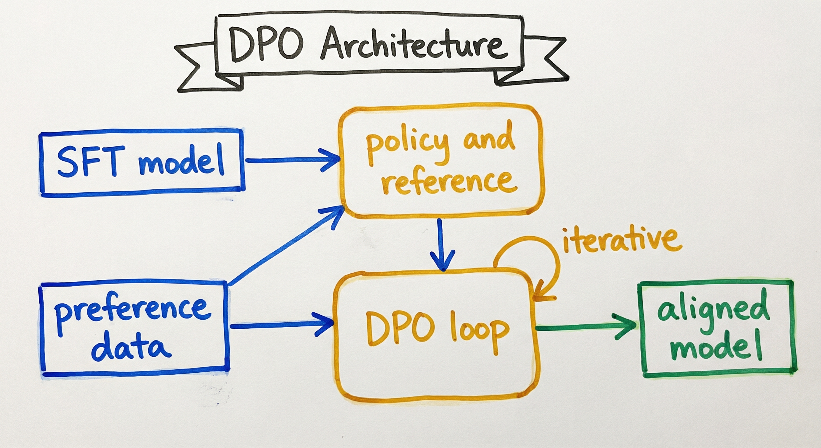
The architecture is deliberately minimalist. The preference dataset contains triples of (prompt, chosen response, rejected response). During each training step, the policy and reference model both compute log-probabilities for the chosen and rejected responses. The DPO loss is computed from the log-probability ratios, and gradients flow only through the policy model. The reference model remains frozen throughout training.
Key Components
Reference Model (Frozen)
An exact copy of the SFT model, kept frozen (no gradient updates) throughout DPO training. It serves as the baseline against which the policy's changes are measured. The implicit reward for any response is the log-ratio of the policy probability to the reference probability. Without the reference model, DPO would have no anchor and the policy could collapse to degenerate solutions. The reference model consumes GPU memory but requires no gradient computation, so it can be loaded in half-precision or even quantized.
Policy Model (Trainable)
The model being optimized. It starts as a copy of the SFT model and is updated via gradient descent on the DPO loss. During training, the policy learns to increase the probability of chosen responses and decrease the probability of rejected responses, relative to what the reference model would assign. After training, this becomes the deployed aligned model.
Preference Dataset
A collection of (prompt, chosen_response, rejected_response) triples. Each triple represents a single human (or AI) preference judgment: given the prompt, the chosen response is preferred over the rejected response. Common sources include human annotation (expensive, high quality), AI feedback from stronger models (cheaper, scalable), and rejection sampling from the policy itself. Datasets are typically formatted in the TRL preference format with chosen and rejected columns.
Log-Probability Computation
Both the policy and reference model compute the per-token log-probabilities for the chosen and rejected responses. These are summed across tokens to get sequence-level log-probabilities: . The log-ratios form the core of the DPO loss.
DPO Loss Function
Computes the binary cross-entropy style loss: . This is a simple, differentiable scalar loss that drives the policy toward preferring chosen responses. The parameter scales the log-ratios, controlling the effective learning rate and regularization strength.
Evaluation Pipeline
After DPO training, the aligned model is evaluated on preference benchmarks: MT-Bench (multi-turn dialogue, scored by GPT-4 judge), AlpacaEval (single-turn, win-rate against a reference model), and IFEval (instruction-following with verifiable constraints). Reward model scores and human evaluations may also be used. If performance is insufficient, the loop iterates with new preference data.
Data Flow
Here's the end-to-end data flow for DPO alignment:
Phase 1: Data Preparation. Start with a preference dataset. Each example contains a prompt, a chosen response, and a rejected response. The data may come from human annotations, AI feedback (e.g., GPT-4 ranking model outputs), or rejection sampling (generate multiple responses from the SFT model, rank them, pair the best with the worst). Format the data into the standard TRL preference format.
Phase 2: Forward Pass. For each batch, compute the log-probabilities of both the chosen and rejected responses under both the policy model and the reference model. This requires four forward passes per batch (policy on chosen, policy on rejected, reference on chosen, reference on rejected). In practice, the reference model forward passes can be precomputed and cached.
Phase 3: Loss Computation and Backward Pass. Compute the DPO loss from the four sets of log-probabilities. Backpropagate gradients through the policy model only. Update policy weights via AdamW optimizer.
Phase 4: Evaluation and Iteration. After training (typically 1-3 epochs), evaluate on MT-Bench, AlpacaEval, and domain-specific benchmarks. If iterating (online DPO), generate new responses from the updated policy, collect new preference judgments, and repeat from Phase 1.
A directed flow showing: the SFT Model is copied into both a Frozen Reference Model and a Trainable Policy Model. The Preference Dataset feeds into the DPO Training Loop along with both model copies. The loop produces a DPO-Aligned Model, which is evaluated. If iteration is needed, new preferences are generated and fed back into the loop. Otherwise, the model is deployed.
How to Implement
Practical Implementation Approaches
DPO implementation is significantly simpler than RLHF. The entire training loop can be written in about 100 lines of PyTorch, and production-grade implementations are available in HuggingFace TRL, Axolotl, and OpenRLHF.
Tier 1: Full-parameter DPO -- Update all weights of the policy model. Requires loading two full model copies (policy + reference) in memory. For a 7B model in bf16, this means ~28GB for both models plus ~14GB for optimizer states, totaling ~42GB -- feasible on a single A100 80GB or 2x A100 40GB. Meta used this approach for Llama 3.
Tier 2: LoRA/QLoRA DPO -- Apply LoRA adapters to the policy model while keeping the base weights frozen. The reference model is the frozen base weights, so you don't need a separate reference model copy. This dramatically reduces memory: a 7B model with QLoRA DPO fits on a single RTX 4090 (24GB). HuggingFace TRL's DPOTrainer supports this natively.
Tier 3: Reference-free DPO variants -- Methods like SimPO and ORPO eliminate the reference model entirely, further reducing memory. SimPO uses length-normalized log-probabilities as the implicit reward; ORPO combines SFT and preference optimization in a single loss. These are the most memory-efficient options.
Cost Context for India: Running full-parameter DPO on a 7B model on a single A100 80GB costs approximately 6-24 (~INR 500-2,000). With QLoRA DPO on an RTX 4090, the same run costs 2-8 (~INR 170-670). Indian cloud providers like E2E Networks and Jarvislabs.ai offer A100s at 30-40% lower cost than AWS. The most expensive part is often the preference data: human annotation of 10K preference pairs costs 500-1,500 (~INR 42,000-1.25 lakh) for the same volume.
from datasets import load_dataset
from transformers import AutoModelForCausalLM, AutoTokenizer
from trl import DPOConfig, DPOTrainer
from peft import LoraConfig

# Load the SFT model and tokenizer
model_name = "meta-llama/Llama-2-7b-chat-hf"
tokenizer = AutoTokenizer.from_pretrained(model_name)
tokenizer.pad_token = tokenizer.eos_token

model = AutoModelForCausalLM.from_pretrained(
    model_name,
    torch_dtype="auto",
    device_map="auto",
)

# The reference model is created automatically by DPOTrainer
# as a frozen copy of the initial model

# Load preference dataset (chosen/rejected format)
dataset = load_dataset("trl-lib/ultrafeedback_binarized", split="train")

# Optional: LoRA for memory efficiency
lora_config = LoraConfig(
    r=16,
    lora_alpha=32,
    lora_dropout=0.05,
    target_modules=["q_proj", "k_proj", "v_proj", "o_proj"],
    task_type="CAUSAL_LM",
)

# DPO training configuration
training_args = DPOConfig(
    output_dir="./llama2-7b-dpo",
    beta=0.1,                         # KL penalty coefficient
    num_train_epochs=1,
    per_device_train_batch_size=2,
    gradient_accumulation_steps=8,
    learning_rate=5e-7,               # Lower LR than SFT
    lr_scheduler_type="cosine",
    warmup_ratio=0.1,
    bf16=True,
    logging_steps=10,
    save_strategy="steps",
    save_steps=500,
    max_length=1024,                  # Max combined length
    max_prompt_length=512,            # Max prompt length
    loss_type="sigmoid",              # Standard DPO loss
    gradient_checkpointing=True,
)

# Create DPO trainer
trainer = DPOTrainer(
    model=model,
    args=training_args,
    train_dataset=dataset,
    processing_class=tokenizer,
    peft_config=lora_config,  # Remove this line for full fine-tuning
)

# Train
trainer.train()
trainer.save_model("./llama2-7b-dpo-final")
This demonstrates the standard DPO training workflow using HuggingFace TRL. Key decisions explained: (1) beta=0.1 is the standard starting point -- it provides moderate regularization against the reference model; (2) learning_rate=5e-7 is much lower than SFT learning rates (typically 2e-4 for LoRA SFT) because DPO is fine-tuning an already-capable model and aggressive updates cause instability; (3) loss_type="sigmoid" selects standard DPO -- TRL also supports "ipo", "kto", and other variants; (4) the reference model is created automatically as a frozen copy of the initial model. With LoRA, the frozen base weights are the reference model, saving significant memory.
import torch
import torch.nn.functional as F
from typing import Tuple

def compute_dpo_loss(
    policy_chosen_logps: torch.Tensor,
    policy_rejected_logps: torch.Tensor,
    reference_chosen_logps: torch.Tensor,
    reference_rejected_logps: torch.Tensor,
    beta: float = 0.1,
) -> Tuple[torch.Tensor, torch.Tensor, torch.Tensor]:
    """
    Compute the DPO loss given log-probabilities from policy and reference models.

    Args:
        policy_chosen_logps: Log P(chosen | prompt) under the policy model
        policy_rejected_logps: Log P(rejected | prompt) under the policy model
        reference_chosen_logps: Log P(chosen | prompt) under the reference model
        reference_rejected_logps: Log P(rejected | prompt) under the reference model
        beta: KL penalty coefficient (higher = more conservative)

    Returns:
        loss: Scalar DPO loss
        chosen_rewards: Implicit rewards for chosen responses
        rejected_rewards: Implicit rewards for rejected responses
    """
    # Compute log-ratios (implicit rewards)
    chosen_rewards = beta * (policy_chosen_logps - reference_chosen_logps)
    rejected_rewards = beta * (policy_rejected_logps - reference_rejected_logps)

    # DPO loss: -log sigmoid(reward_chosen - reward_rejected)
    logits = chosen_rewards - rejected_rewards
    loss = -F.logsigmoid(logits).mean()

    return loss, chosen_rewards.detach(), rejected_rewards.detach()


def get_sequence_log_probs(
    model, input_ids: torch.Tensor, attention_mask: torch.Tensor, labels: torch.Tensor
) -> torch.Tensor:
    """
    Compute per-sequence log-probability: sum of log P(token_t | tokens_<t).
    Labels should have -100 for prompt tokens (only count response tokens).
    """
    with torch.no_grad() if not model.training else torch.enable_grad():
        outputs = model(input_ids=input_ids, attention_mask=attention_mask)
        logits = outputs.logits[:, :-1, :]  # Shift for causal LM
        labels = labels[:, 1:]               # Shift labels

        # Per-token log probabilities
        log_probs = F.log_softmax(logits, dim=-1)
        token_log_probs = torch.gather(
            log_probs, dim=-1, index=labels.unsqueeze(-1)
        ).squeeze(-1)

        # Mask out prompt tokens (labeled as -100)
        mask = (labels != -100).float()
        sequence_log_probs = (token_log_probs * mask).sum(dim=-1)

    return sequence_log_probs


# Example usage
batch_size = 4
# In practice, these come from forward passes through policy and reference models
policy_chosen = torch.randn(batch_size)    # log P_policy(chosen | prompt)
policy_rejected = torch.randn(batch_size)  # log P_policy(rejected | prompt)
ref_chosen = torch.randn(batch_size)       # log P_ref(chosen | prompt)
ref_rejected = torch.randn(batch_size)     # log P_ref(rejected | prompt)

loss, chosen_r, rejected_r = compute_dpo_loss(
    policy_chosen, policy_rejected, ref_chosen, ref_rejected, beta=0.1
)
print(f"DPO Loss: {loss.item():.4f}")
print(f"Mean chosen reward: {chosen_r.mean().item():.4f}")
print(f"Mean rejected reward: {rejected_r.mean().item():.4f}")
print(f"Reward margin: {(chosen_r - rejected_r).mean().item():.4f}")
This educational implementation shows the DPO loss from first principles. The compute_dpo_loss function takes pre-computed log-probabilities and returns the loss plus the implicit rewards for monitoring. The get_sequence_log_probs function shows how to extract sequence-level log-probabilities from a causal LM, with proper label masking. In production, you would use TRL's DPOTrainer which handles all of this, but understanding the raw computation is essential for debugging. The reward margin (chosen_reward - rejected_reward) is the most important metric to monitor during training: it should increase steadily and plateau.
import torch
from transformers import AutoModelForCausalLM, AutoTokenizer
from datasets import Dataset
import json
from typing import List, Dict

def generate_rejection_sampling_data(
    model_name: str,
    prompts: List[str],
    n_samples: int = 8,
    reward_model_name: str = "OpenAssistant/reward-model-deberta-v3-large-v2",
    temperature: float = 0.8,
    max_new_tokens: int = 512,
) -> List[Dict]:
    """
    Generate preference pairs via rejection sampling:
    1. Generate N responses per prompt from the SFT model
    2. Score each response with a reward model
    3. Pair the highest-scored (chosen) with lowest-scored (rejected)
    """
    # Load generation model
    tokenizer = AutoTokenizer.from_pretrained(model_name)
    tokenizer.pad_token = tokenizer.eos_token
    model = AutoModelForCausalLM.from_pretrained(
        model_name, torch_dtype=torch.bfloat16, device_map="auto"
    )

    preference_data = []

    for prompt in prompts:
        inputs = tokenizer(prompt, return_tensors="pt").to(model.device)

        # Generate N candidate responses
        responses = []
        for _ in range(n_samples):
            output = model.generate(
                **inputs,
                max_new_tokens=max_new_tokens,
                temperature=temperature,
                do_sample=True,
                top_p=0.9,
            )
            response_text = tokenizer.decode(
                output[0][inputs["input_ids"].shape[1]:],
                skip_special_tokens=True,
            )
            responses.append(response_text)

        # Score responses (simplified; use actual reward model in production)
        # Here we use length-adjusted diversity as a proxy
        scores = []
        for resp in responses:
            # In production, replace with reward model scoring:
            # score = reward_model(prompt, resp)
            score = len(set(resp.split())) / max(len(resp.split()), 1)  # proxy
            scores.append(score)

        # Pair best with worst
        best_idx = max(range(len(scores)), key=lambda i: scores[i])
        worst_idx = min(range(len(scores)), key=lambda i: scores[i])

        if best_idx != worst_idx:
            preference_data.append({
                "prompt": prompt,
                "chosen": responses[best_idx],
                "rejected": responses[worst_idx],
                "chosen_score": scores[best_idx],
                "rejected_score": scores[worst_idx],
            })

    return preference_data

# Example usage
prompts = [
    "Explain how gradient descent works in simple terms.",
    "Write a Python function to find the longest common subsequence.",
    "What are the key differences between TCP and UDP?",
]

preference_pairs = generate_rejection_sampling_data(
    model_name="meta-llama/Llama-2-7b-chat-hf",
    prompts=prompts,
    n_samples=8,
)

# Convert to HuggingFace dataset for DPOTrainer
dataset = Dataset.from_list(preference_pairs)
print(f"Generated {len(dataset)} preference pairs")
print(f"Example chosen score: {preference_pairs[0]['chosen_score']:.3f}")
print(f"Example rejected score: {preference_pairs[0]['rejected_score']:.3f}")
This shows how to create preference data via rejection sampling, a technique used by Meta for Llama 3 and by many teams as a cheaper alternative to human annotation. The idea: generate multiple candidate responses from the SFT model, score them with a reward model (or heuristic), and pair the best with the worst. This creates on-policy preference data since the responses come from the model being aligned. In production, replace the proxy scoring with an actual reward model like OpenAssistant/reward-model-deberta-v3-large-v2 or use GPT-4 as a judge. Generating 60K preference pairs this way costs approximately 15,000-30,000 for human annotation (~INR 12.5-25 lakh).
# Axolotl configuration for DPO training (YAML)
base_model: meta-llama/Llama-2-7b-chat-hf
model_type: LlamaForCausalLM
tokenizer_type: LlamaTokenizer

load_in_8bit: false
load_in_4bit: true        # QLoRA for memory efficiency

adapter: lora
lora_r: 16
lora_alpha: 32
lora_dropout: 0.05
lora_target_modules:
  - q_proj
  - k_proj
  - v_proj
  - o_proj

# DPO-specific settings
rl: dpo
dpo_beta: 0.1             # KL penalty coefficient

datasets:
  - path: argilla/ultrafeedback-binarized-preferences
    type: chatml.intel
    split: train

sequence_len: 2048
val_set_size: 0.02

gradient_accumulation_steps: 8
micro_batch_size: 2
num_epochs: 1
learning_rate: 5e-7
lr_scheduler: cosine
warmup_ratio: 0.1
optimizer: adamw_torch
weight_decay: 0.0

bf16: true
tf32: true
gradient_checkpointing: true

save_strategy: steps
save_steps: 500
evaluation_strategy: steps
eval_steps: 100

wandb_project: dpo-alignment
wandb_run_id: llama2-7b-dpo-v1
Common Implementation Mistakes
- ●
Learning rate too high: DPO is far more sensitive to learning rate than SFT. Using SFT-level learning rates (2e-4) will cause the policy to diverge from the reference model catastrophically. Start with 5e-7 for full fine-tuning or 5e-6 for LoRA, and only increase if the reward margin is not growing.
- ●
Ignoring the reference model memory cost: Beginners often forget that DPO requires keeping the reference model in memory alongside the policy model, effectively doubling memory requirements compared to SFT. Use LoRA (where the frozen base weights serve as the reference) or quantize the reference model to mitigate this.
- ●
Training for too many epochs: DPO typically converges within 1-2 epochs. Training for 5+ epochs causes severe overfitting to the preference dataset, where the model memorizes specific preferred phrases rather than learning general alignment. Monitor eval loss and the reward margin plateau.
- ●
Low-quality preference data: DPO is garbage-in, garbage-out. If the chosen and rejected responses are barely different in quality, or if preference labels are noisy (>15% label noise), DPO will not learn meaningful alignment. Invest in data quality: filter for high reward-margin pairs where the quality difference is clear.
- ●
Not monitoring implicit rewards: The chosen and rejected implicit rewards (log-ratios) should be tracked during training. The reward margin (chosen - rejected) should increase and plateau. If chosen rewards increase but rejected rewards also increase, the model is not learning to discriminate -- likely a data quality issue.
- ●
Forgetting to use the same chat template: The policy, reference model, and preference data must all use the same chat template. A template mismatch causes the reference model's log-probabilities to be meaningless, breaking the implicit reward signal.
When Should You Use This?
Use When
You have an SFT-tuned model and want to align it to human preferences without the complexity of training a reward model and running PPO
You have a preference dataset of (prompt, chosen, rejected) triples -- either from human annotation, AI feedback, or rejection sampling
You want a stable, reproducible alignment process that is easy to debug and iterate on, without RL hyperparameter sensitivity
Your compute budget is limited -- DPO requires roughly half the GPU memory of PPO-based RLHF (2 models instead of 4)
You are aligning an open-source model (Llama, Mistral, Qwen) and want a well-tested alignment recipe with strong community tooling support
You need to iterate quickly on alignment -- DPO training runs in 2-4 hours for a 7B model, enabling rapid experimentation with different preference datasets
Avoid When
You have only positive examples (no rejected responses) -- DPO requires paired preferences. Consider KTO instead, which works with binary (good/bad) labels without pairing
Your preference data has high label noise (>20% of labels are incorrect) -- DPO is sensitive to noisy preferences. Consider cDPO or IPO which handle noise more gracefully
You need the model to improve beyond what the preference data demonstrates -- DPO is offline and bounded by data quality. Online RL methods (PPO, GRPO) can potentially discover better responses through exploration
You are aligning a very large model (70B+) where the cost of loading two model copies is prohibitive -- consider reference-free methods like SimPO or ORPO
The chosen and rejected responses in your data are very similar in quality -- DPO needs clear quality separation to learn meaningful preferences. If the reward margin in your data is small, DPO will learn noise
You want to combine SFT and preference alignment in a single stage -- DPO assumes a pre-existing SFT model. Consider ORPO which merges both stages
Key Tradeoffs
DPO vs. RLHF (PPO)
The fundamental tradeoff is simplicity vs. flexibility. DPO is dramatically simpler to implement and more stable to train, but it is an offline method -- it optimizes over a fixed preference dataset without generating new responses during training. PPO-based RLHF is online -- it generates responses during training and gets reward feedback, enabling it to explore beyond the training data distribution.
| Dimension | DPO | RLHF (PPO) |
|---|---|---|
| Models in memory | 2 (policy + reference) | 4 (policy + reference + reward + value) |
| GPU memory (7B model) | ~42GB | ~84GB |
| Implementation complexity | ~100 lines | ~1,000+ lines |
| Hyperparameter sensitivity | Low (mainly beta, LR) | High (PPO clip, GAE lambda, KL coeff, etc.) |
| Training stability | High | Moderate (reward hacking, mode collapse) |
| Exploration ability | None (offline) | High (on-policy generation) |
| Ceiling quality | Bounded by preference data | Can exceed preference data quality |
| Compute cost (7B, 60K examples) | $10-25 (~INR 840-2,100) | $40-100 (~INR 3,360-8,400) |
Offline vs. Online DPO
Standard DPO is offline: it trains on a fixed dataset of preference pairs. Online DPO (also called iterative DPO) generates new responses from the policy at each iteration, collects new preference judgments (from humans or AI), and trains on the fresh data. Online DPO addresses the distribution shift problem of offline DPO but adds complexity and cost. Meta used iterative DPO for Llama 3, alternating between data collection and DPO training rounds.
Data Quality vs. Data Quantity
DPO is more sensitive to data quality than data quantity. A dataset of 10K high-margin preference pairs (where chosen is clearly better than rejected) typically outperforms 100K noisy pairs. The Zephyr team showed that filtering the UltraFeedback dataset by GPT-4 scores before DPO training significantly improved the resulting model. For Indian teams on a budget, investing in AI feedback quality (using GPT-4 or Claude as judges) provides better ROI than collecting more human annotations.
Alternatives & Comparisons
RLHF with PPO is the original preference alignment method. It is more complex (4 models, RL hyperparameters) but enables online exploration -- the policy generates responses and receives reward feedback during training. Choose RLHF over DPO when you need the model to discover responses better than what's in your dataset, or when you have a high-quality reward model. Choose DPO when you want simplicity, stability, and lower compute cost.
ORPO combines SFT and preference optimization into a single training stage, eliminating the need for a separate SFT step and a reference model. This makes it the most memory-efficient option. Choose ORPO when you want a single-stage pipeline from base model to aligned model. Choose DPO when you already have an SFT model and want maximum control over each stage.
Reward modeling trains a separate model to score response quality, which is then used as the reward signal for PPO-based RLHF. DPO bypasses reward modeling entirely by defining an implicit reward through the policy's log-ratios. Choose explicit reward modeling when you need the reward model for other purposes (e.g., rejection sampling, best-of-N selection, data filtering). Choose DPO when alignment is the only goal.
Constitutional AI uses a set of principles (the 'constitution') to generate AI feedback for self-improvement, reducing dependence on human annotations. It combines SFT on AI-revised responses (SL-CAI) with RL from AI feedback (RL-CAI). Choose Constitutional AI when you prioritize safety alignment with minimal human annotation. Choose DPO when you have existing preference data and want a simpler optimization procedure.
Instruction tuning is the prerequisite for DPO, not a replacement. SFT teaches the model to follow instructions using supervised learning on demonstrations; DPO then refines the SFT model's behavior using preference data. You almost always need SFT before DPO. The one exception is ORPO, which combines both stages.
Pros, Cons & Tradeoffs
Advantages
Dramatically simpler than RLHF: No reward model to train, no PPO hyperparameters to tune, no value function to estimate. The entire training loop is a single binary cross-entropy-style loss, implementable in ~100 lines of PyTorch.
Lower compute and memory requirements: DPO needs only 2 models in memory (policy + reference) versus 4 for PPO-RLHF. This halves GPU memory requirements and reduces training cost by 50-75%.
Training stability: DPO uses standard gradient descent on a well-behaved loss function, avoiding the instability of RL optimization. No reward hacking through mode collapse, no catastrophic forgetting from aggressive PPO updates.
Theoretically grounded: DPO is provably equivalent to RLHF under the Bradley-Terry preference model -- it produces the same optimal policy. This is not a heuristic approximation; it is an exact reparameterization.
Excellent tooling and community support: HuggingFace TRL's DPOTrainer, Axolotl, OpenRLHF, and NeMo Aligner all provide production-grade DPO implementations. The technique is battle-tested on models from 1B to 405B parameters.
Fast iteration cycles: A DPO training run on a 7B model with 60K preference pairs completes in 2-4 hours on a single A100, enabling rapid experimentation with different datasets and hyperparameters.
Compatible with LoRA/QLoRA: DPO works naturally with parameter-efficient methods. With LoRA, the frozen base weights serve as the reference model for free, eliminating the need to load a separate reference copy.
Disadvantages
Offline limitation: Standard DPO trains on a fixed dataset of preference pairs without generating new responses. This means it cannot discover responses better than what's in the training data, unlike online RL methods that explore the response space.
Distribution shift vulnerability: If the preference data was generated by a model very different from the SFT model (e.g., preferences collected from GPT-4 outputs but applied to a Mistral model), the implicit reward signal becomes unreliable due to distribution mismatch.
Length hacking: DPO can learn a shortcut where the model simply generates longer responses to increase log-probability under the policy, since longer responses tend to have higher reward margin. This is a well-documented failure mode that SimPO specifically addresses.
Sensitive to data quality: DPO amplifies whatever signal is in the preference data. If preferences are noisy, biased, or reflect superficial features (formatting over substance), the aligned model will learn those biases. Garbage in, garbage out.
Beta sensitivity: The beta parameter significantly affects results, and the optimal value varies by model, dataset, and use case. Too low causes over-optimization; too high causes under-fitting. There is no universal default.
Requires preference pairs: DPO needs paired comparisons (chosen vs. rejected for the same prompt), which are more expensive and harder to collect than binary labels (good/bad). Methods like KTO relax this requirement.
Failure Modes & Debugging
Distribution shift between preference data and policy
Cause
The preference data was generated by a model with a very different output distribution than the SFT model being aligned. For example, using GPT-4-generated preferences to align a 7B model, or using preference data from an older model version. The implicit reward derived from the reference model's log-probabilities becomes miscalibrated because the reference model assigns very low probability to the preference data responses.
Symptoms
The DPO loss decreases normally during training, but evaluation metrics (MT-Bench, AlpacaEval) do not improve or actually degrade. The model may become repetitive or produce generic outputs. The implicit reward margin increases but doesn't correlate with actual response quality.
Mitigation
Use on-policy preference data wherever possible: generate responses from the SFT model itself, then rank them. If using off-policy data (from a different model), filter for examples where both chosen and rejected responses have reasonable probability under the reference model. Online/iterative DPO (generating fresh responses each round) addresses this most directly.
Length hacking / verbosity bias
Cause
The DPO loss uses sequence-level log-probabilities, which naturally scale with response length (longer responses accumulate more log-probability mass). If the chosen responses in the preference data tend to be longer than rejected ones -- which is common because human annotators often prefer more detailed answers -- the model learns that length itself is the preferred feature.
Symptoms
The aligned model produces significantly longer responses than the SFT model, often with redundant information, excessive hedging, or filler text. Response quality as judged by humans may actually decrease despite improvements on automated metrics. The average response length increases 2-5x during training.
Mitigation
Use length-normalized log-probabilities instead of raw sequence-level log-probabilities: divide by the number of response tokens. SimPO implements this natively. Alternatively, filter the preference dataset to ensure chosen and rejected responses have similar lengths, or add an explicit length penalty to the loss. TRL's DPOTrainer supports a reference_free mode that helps with this.
Reward over-optimization (implicit reward hacking)
Cause
Training for too many steps or with too low a beta value, causing the policy to drift far from the reference model. The implicit reward increases without bound, but the actual response quality plateaus or degrades because the model is exploiting artifacts of the log-probability ratio rather than genuinely improving.
Symptoms
The reward margin (chosen - rejected implicit rewards) continues to grow without plateauing. Evaluation metrics improve initially then degrade. The model's outputs become increasingly different from the SFT model in style (more verbose, more formulaic, or more sycophantic). KL divergence from the reference model grows rapidly.
Mitigation
Use early stopping based on evaluation metrics (not training loss). Increase beta to tighten the KL constraint. Train for only 1 epoch as a starting point. Monitor the KL divergence between the policy and reference model -- if it exceeds 5-10 nats, the policy has likely drifted too far. Consider IPO, which converges to a bounded solution rather than pushing probabilities to the extremes.
Preference label noise causing degenerate learning
Cause
The preference dataset contains a significant fraction (>15%) of incorrectly labeled pairs -- where the 'chosen' response is actually worse than the 'rejected' response. This is common with crowdsourced annotations, subjective tasks, and noisy AI feedback. DPO's sigmoid loss amplifies confident mis-labels.
Symptoms
The model learns contradictory preferences, producing outputs that are inconsistent in quality. On some prompts it improves, on others it actively degrades. The training loss may oscillate rather than decrease smoothly. Evaluation results are highly variable across runs.
Mitigation
Use conservative DPO (cDPO) which adds label smoothing to account for noise. The cDPO loss assumes a fraction of labels are flipped and adjusts accordingly. In TRL, set loss_type="sigmoid" with label_smoothing=0.1. Alternatively, use IPO which is theoretically robust to label noise. Pre-filter the dataset by removing examples where an external reward model assigns similar scores to both responses.
Catastrophic forgetting of SFT capabilities
Cause
Overly aggressive DPO training (low beta, high learning rate, many epochs) causes the model to lose instruction-following capabilities learned during SFT. The model optimizes so aggressively for the preference signal that it forgets how to follow basic instructions or generates incoherent text.
Symptoms
The model scores well on preference benchmarks but poorly on instruction-following benchmarks (IFEval). It may refuse reasonable requests, generate truncated responses, or lose multilingual capabilities. MMLU and other knowledge benchmarks degrade significantly.
Mitigation
Use conservative hyperparameters: beta >= 0.1, learning rate <= 5e-7 (full FT) or 5e-6 (LoRA), 1 epoch maximum. Monitor capability retention benchmarks (MMLU, ARC, IFEval) alongside preference metrics. Use LoRA to limit the number of parameters that change. If using full fine-tuning, consider mixing in a small fraction (5-10%) of SFT data during DPO training to prevent forgetting.
Placement in an ML System
Where DPO Sits in the ML System
DPO occupies the alignment stage of the LLM training pipeline, directly after supervised fine-tuning:
- Pretraining: Self-supervised next-token prediction on trillions of tokens. Gives the model knowledge and linguistic ability.
- Supervised Fine-Tuning (SFT): Train on instruction-response pairs to teach the model to follow instructions.
- DPO Alignment: Train on preference pairs to align the model's outputs with human preferences -- making responses more helpful, harmless, and honest.
- Optional: Further refinement via rejection sampling, best-of-N selection, or iterative DPO.
DPO replaces stages 2 and 3 of the original RLHF pipeline (reward model training + PPO optimization) with a single DPO training run. The SFT stage (stage 1 of RLHF) is still required as a prerequisite.
In production deployment, the DPO-aligned model is typically the final model served to users. Some teams apply additional post-processing: safety classifiers, output filtering, or best-of-N selection using a reward model at inference time. For Indian companies building production LLM applications -- whether Krutrim aligning multilingual models, startups building domain-specific copilots, or enterprises at Infosys and Wipro deploying internal AI assistants -- DPO is the standard alignment recipe for its simplicity and effectiveness.
Pipeline Stage
Training / Alignment
Upstream
- instruction-tuning
- full-fine-tuning
- lora-fine-tuning
Downstream
- knowledge-distillation
- model-registry
Scaling Bottlenecks
The primary scaling bottleneck is GPU memory: DPO requires two model copies (policy + reference). For a 7B model in bf16, this is ~28GB just for parameters, plus ~14GB for optimizer states, totaling ~42GB. A 70B model requires ~280GB for both copies, necessitating multi-GPU setups with model parallelism. Solutions: QLoRA DPO (reference = frozen base weights, no extra copy needed), quantized reference model (load reference in 4-bit), or gradient checkpointing.
Collecting high-quality preference data is the bottleneck for most teams. Human annotation scales linearly in cost: 10K pairs costs $10,000-30,000 (~INR 8.4-25 lakh). AI feedback is cheaper but introduces distribution shift. Rejection sampling requires significant inference compute (8 generations per prompt). The most scalable approach is iterative: start with AI feedback, DPO-align, rejection-sample from the improved model, and repeat.
For online/iterative DPO, the bottleneck shifts to inference throughput during the data collection phase. Generating 60K preference pairs via rejection sampling (8 samples per prompt for 7.5K prompts) at 512 tokens per response requires approximately 240M tokens of generation -- about 4-8 hours on a single A100 with vLLM. This means each iteration cycle (data collection + DPO training) takes roughly 8-12 hours.
Production Case Studies
Meta's Llama 3.1 post-training methodology combines Supervised Fine-Tuning (SFT), Rejection Sampling (RS), and Direct Preference Optimization (DPO). Each alignment round uses DPO to improve model performance on reasoning and coding tasks without requiring a separate rewards model.
Learning from preference rankings via PPO and DPO greatly improved Llama 3's performance on reasoning and coding tasks. For Llama 3.1, each round of alignment involves SFT, RS, and DPO, making it Meta's most capable openly available LLM to date.
HuggingFace's Zephyr-7B was one of the first high-profile demonstrations of DPO for open-source model alignment. The team applied distilled DPO (dDPO) to a Mistral-7B model that had been SFT-tuned on the UltraChat dataset. Preference data came from GPT-4 scoring of the UltraFeedback dataset, with no human annotation required.
Zephyr-7B-beta achieved the highest MT-Bench score among 7B models at its release, surpassing even Llama-2-Chat-70B (a model 10x larger that used PPO-based RLHF). The project demonstrated that DPO with AI feedback could match or exceed PPO-RLHF with human feedback, at a fraction of the cost -- training took only a few hours on 16 A100 GPUs.
DeepSeek used DPO alongside their novel GRPO algorithm for DeepSeekMath, a 7B model specialized in mathematical reasoning. They compared DPO, PPO, and GRPO on math benchmarks and provided a unified analysis showing that DPO and GRPO can be understood as simplified RL methods within the same theoretical framework.
DeepSeekMath-7B achieved 51.7% on the competition-level MATH benchmark, approaching GPT-4 and Gemini-Ultra performance. While GRPO slightly outperformed DPO on math tasks, DPO was used as a strong baseline and showed competitive results with significantly simpler implementation. The work influenced DeepSeek's subsequent model development.
The Princeton NLP group developed SimPO, a reference-free variant of DPO that uses length-normalized average log-probability as the implicit reward, addressing DPO's length bias and reference model dependency. SimPO was applied to Llama 3 8B Instruct and Mistral 7B Instruct models.
SimPO outperformed DPO by 3.6 to 4.8 points on AlpacaEval 2 LC win rate across various settings, while using less memory (no reference model needed) and being simpler to implement. The work was published at NeurIPS 2024 and became a popular alternative for teams seeking memory-efficient alignment.
Tooling & Ecosystem
HuggingFace's official library for LLM alignment. The DPOTrainer is the most widely used DPO implementation, supporting standard DPO, IPO, KTO, cDPO, and other variants via the loss_type parameter. Features include automatic reference model creation, LoRA/QLoRA support, dataset formatting utilities, and integration with Weights & Biases for experiment tracking. Used to train Zephyr, Notus, and many other aligned models.
A comprehensive fine-tuning framework that supports DPO, IPO, KTO, ORPO, and GRPO via YAML configuration. Configuration-driven approach with rl: dpo and dpo_beta: 0.1 settings. Supports all major model architectures (Llama, Mistral, Qwen, Phi) and PEFT methods. Ideal for reproducible DPO experiments.
A scalable RLHF and DPO framework built on Ray, designed for distributed training on hundreds of GPUs. Supports DPO, IPO, cDPO, and KTO alongside PPO and REINFORCE++. Distributes policy, reference, and reward models across separate GPU groups for efficient memory utilization. Can fine-tune 70B+ models across multiple A100 nodes.
NVIDIA's enterprise-grade alignment toolkit with highly optimized DPO, PPO, and SteerLM implementations. Features tensor parallelism, pipeline parallelism, and expert parallelism for training at scale. Provides production-ready training recipes for DPO alignment of models from 7B to 340B parameters.
The official reference implementation from the DPO paper authors (Eric Mitchell et al.). Clean, minimal PyTorch code that implements the core DPO algorithm. Useful for understanding the method from first principles, though production use cases should prefer TRL or Axolotl for robustness and features.
A unified fine-tuning framework with a web UI, supporting DPO, ORPO, KTO, and other alignment methods for 100+ LLMs. Offers a particularly accessible interface for DPO training: select the model, upload preference data, configure beta and learning rate via the UI, and launch training. Popular in the Asian and Indian ML communities for its ease of use.
Research & References
Rafailov, Sharma, Mitchell, Ermon, Manning & Finn (2023)NeurIPS 2023
The foundational DPO paper. Showed that the RLHF objective can be reparameterized to eliminate the reward model, yielding a simple classification loss on preference pairs. DPO matched or exceeded PPO-based RLHF on summarization, dialogue, and sentiment control while being substantially simpler to implement and train.
Azar, Rowland, Piot, Guo, Calandriello, Valko & Munos (2023)AISTATS 2024
Introduced the general PO framework that unifies RLHF, DPO, and a new method called IPO (Identity Preference Optimization). IPO uses an MSE-based loss that avoids DPO's failure mode of pushing probabilities to extremes, providing better regularization and robustness to label noise.
Ethayarajh, Xu, Muennighoff, Jurafsky & Kiela (2024)ICML 2024
Proposed KTO (Kahneman-Tversky Optimization), which aligns models using only binary (desirable/undesirable) labels rather than paired preferences. Based on prospect theory from behavioral economics. Matched or exceeded DPO at scales from 1B to 30B parameters while requiring only unpaired data, making it far more practical for real-world deployment.
Meng, Xia & Chen (2024)NeurIPS 2024
Eliminated the reference model by using length-normalized average log-probability as the implicit reward. Added a target reward margin to encourage larger quality separation. SimPO outperformed DPO by 3.6-4.8 points on AlpacaEval 2 while being more compute and memory efficient.
Hong, Lee & Thorne (2024)EMNLP 2024
Combined SFT and preference optimization into a single training stage using an odds-ratio penalty that disfavors rejected responses during SFT. Eliminated both the separate SFT stage and the reference model. ORPO on Mistral-7B achieved competitive results with DPO while requiring half the training stages.
Lai, Tan, Zhongwei, Liu, Yang, Huang, Shang & Jiang (2024)arXiv preprint
Applied DPO at the reasoning-step level rather than the response level for mathematical reasoning tasks. As few as 10K step-level preference pairs yielded a 3% accuracy gain on MATH for 70B+ models, demonstrating that granular preference signals are more effective than holistic response-level DPO for reasoning tasks.
Interview & Evaluation Perspective
Common Interview Questions
- ●
What is DPO and how does it differ from RLHF?
- ●
Derive the DPO loss function from the RLHF objective.
- ●
What is the role of the reference model in DPO? What happens if you remove it?
- ●
Explain the beta parameter and how you would tune it.
- ●
What are the main failure modes of DPO, and how would you address each?
- ●
Compare DPO, IPO, KTO, and SimPO -- when would you choose each?
- ●
How would you design an iterative DPO pipeline for production alignment?
- ●
Why might DPO underperform PPO-RLHF, and when would you switch to PPO?
Key Points to Mention
- ●
DPO is a reparameterization of RLHF, not an approximation. The closed-form solution of the KL-constrained objective under the Bradley-Terry model is what makes the elimination of the reward model mathematically exact.
- ●
The implicit reward is the log-ratio of policy to reference probabilities, scaled by beta. This is the fundamental quantity that DPO optimizes, even though no explicit reward is ever computed.
- ●
The DPO gradient has an intuitive form: it weights each example by how much the model is currently getting it wrong (the sigmoid of the negative reward margin). This provides a natural curriculum effect.
- ●
Distribution shift is the Achilles heel of offline DPO. The preference data should ideally come from the SFT model being aligned (on-policy). Using off-policy data from a very different model leads to miscalibrated implicit rewards.
- ●
Meta used DPO (not PPO) for Llama 3 alignment, finding it more stable and compute-efficient at scale. This is strong industry validation.
- ●
For Indian cost context: DPO alignment of a 7B model costs approximately INR 500-2,000 in compute, compared to INR 3,000-8,000 for PPO-RLHF. The dominant cost is preference data collection, not training compute.
Pitfalls to Avoid
- ●
Claiming DPO is 'better than RLHF' without nuance. DPO is simpler and more stable but is bounded by the quality of offline preference data. PPO can potentially discover better responses through online exploration.
- ●
Forgetting to mention the reference model. DPO without a reference model is not DPO -- it's reward hacking. The reference provides essential regularization.
- ●
Not knowing about DPO variants (IPO, KTO, SimPO). A strong candidate should be able to discuss when each variant is appropriate.
- ●
Confusing DPO with SFT. DPO requires preference pairs (chosen vs. rejected), not demonstrations. The loss function is fundamentally different from cross-entropy on demonstrations.
- ●
Ignoring the data requirements. DPO requires paired preferences, which are harder and more expensive to collect than unpaired labels. This practical constraint is important in system design discussions.
Senior-Level Expectation
A senior/staff candidate should be able to derive the DPO loss from the RLHF objective in 3-4 steps, discuss the gradient analysis showing the natural curriculum effect, and explain why distribution shift is the fundamental challenge. They should design a complete alignment pipeline: SFT -> rejection sampling to generate on-policy responses -> reward model or AI judge to create preference pairs -> DPO training -> evaluation on MT-Bench + IFEval + domain-specific benchmarks -> iteration. They should discuss when to use DPO vs. PPO vs. KTO (based on data availability and quality requirements), how to detect and mitigate length hacking, and the cost-quality tradeoffs between human and AI preference annotation. Familiarity with the Llama 3 alignment recipe (iterative DPO with rejection sampling) and the Zephyr recipe (distilled DPO with AI feedback) demonstrates current industry knowledge. The ability to reason about the beta parameter's effect on the KL constraint and when to use IPO or cDPO for noisy data is a strong staff-level signal.
Summary
Let's recap the key ideas covered in this guide:
Direct Preference Optimization (DPO) is an alignment algorithm that reparameterizes the standard RLHF objective to eliminate the need for a separate reward model and reinforcement learning. By exploiting the closed-form solution of the KL-constrained reward maximization objective under the Bradley-Terry preference model, DPO defines an implicit reward through the log-probability ratio between the trained policy and a frozen reference model. The resulting loss function is a simple binary cross-entropy on preference pairs, trainable with standard gradient descent in ~100 lines of PyTorch.
The DPO training pipeline is dramatically simpler than RLHF: it requires only 2 models in memory (policy + reference) instead of 4, has fewer hyperparameters (mainly beta and learning rate), and is far more stable to train. The beta parameter controls how far the policy can deviate from the reference, with being the most common default. DPO was validated at industry scale when Meta chose it over PPO for Llama 3 alignment, and it became the de facto standard for open-source model alignment after HuggingFace's Zephyr demonstrated that DPO with AI feedback could surpass PPO-RLHF with human feedback.
The DPO family has expanded rapidly: IPO addresses over-optimization with MSE-based loss, KTO eliminates the need for paired preferences, cDPO handles noisy labels, SimPO removes the reference model entirely, and ORPO combines SFT with preference alignment in a single stage. The main limitations of standard DPO are its offline nature (bounded by training data quality), vulnerability to distribution shift between preference data and the model's own outputs, and susceptibility to length hacking. Online/iterative DPO, which alternates between generating new responses and collecting fresh preferences, addresses the distribution shift problem and was the approach Meta used for Llama 3. For teams building production LLM applications -- whether at Indian startups or global tech companies -- DPO provides the best balance of simplicity, stability, and effectiveness for preference alignment.