Full Fine-tuning in Machine Learning
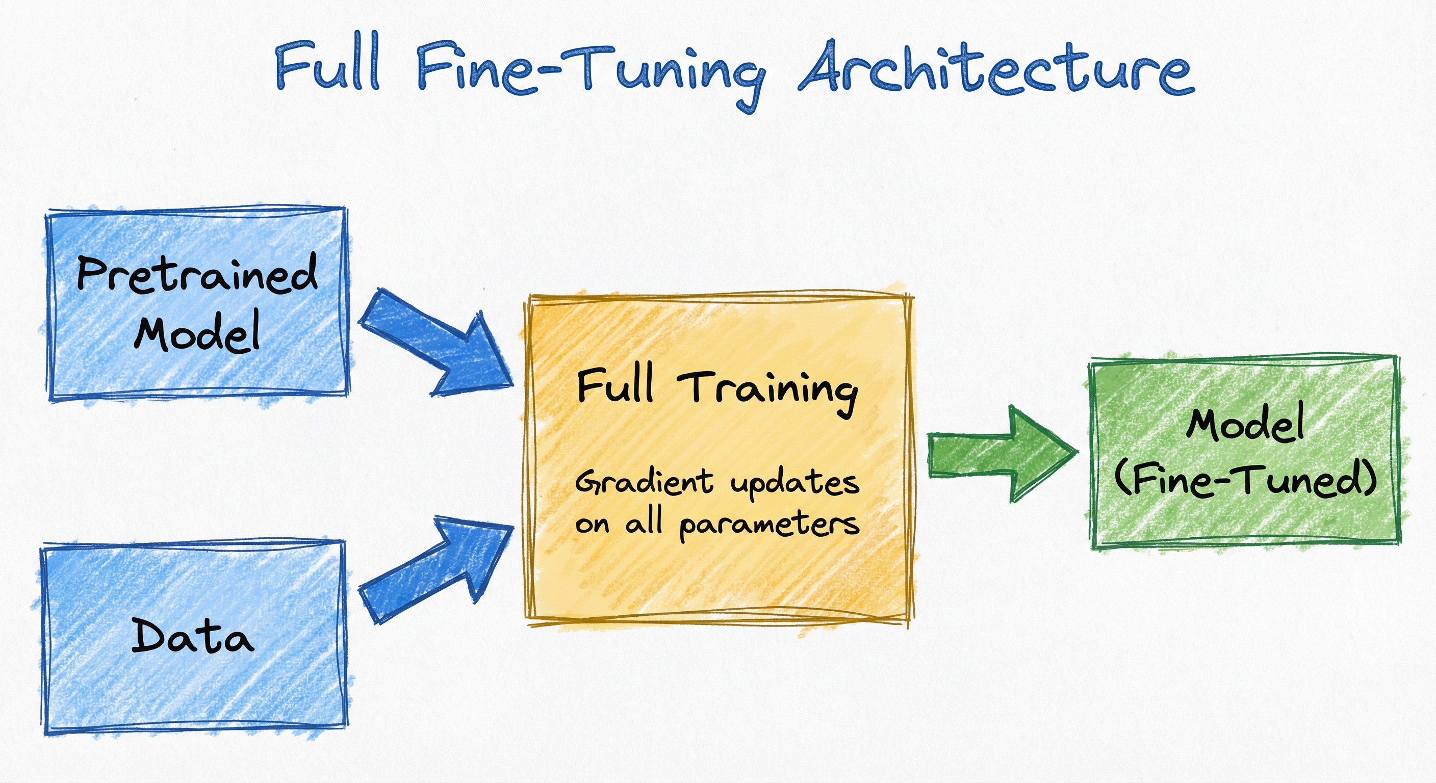
Full fine-tuning is the process of taking a pretrained model and updating every single parameter on your task-specific dataset. No frozen layers, no low-rank approximations, no adapter modules -- every weight in the network is fair game for gradient updates.
This is the oldest and most straightforward form of transfer learning. You start with a model that has already learned rich representations from a massive pretraining corpus, then you reshape those representations to fit your specific task by training on your (typically much smaller) labeled dataset.
Why does this matter so much in 2026? Because the explosion of foundation models -- from BERT to GPT-4 to Llama 3 -- has made fine-tuning the dominant paradigm for building production ML systems. Very few teams pretrain from scratch anymore. The question isn't whether to fine-tune, but how to fine-tune: full parameter updates vs. parameter-efficient methods like LoRA and QLoRA.
Full fine-tuning remains the gold standard for maximum task performance. When you have sufficient compute and data, updating all parameters gives the model the most degrees of freedom to adapt. But it comes with real costs -- GPU memory, training time, catastrophic forgetting risk, and the operational complexity of managing full model checkpoints. Understanding when full fine-tuning is worth those costs, and when a parameter-efficient alternative is the smarter choice, is one of the most important decisions in modern ML system design.
Concept Snapshot
- What It Is
- A transfer learning method that updates all parameters of a pretrained model on a downstream task-specific dataset to maximize task performance.
- Category
- Model Training
- Complexity
- Intermediate
- Inputs / Outputs
- Inputs: pretrained model weights + task-specific labeled dataset. Outputs: a fully adapted model with all parameters updated for the target task.
- System Placement
- Sits after pretraining (or continued pretraining) and before model evaluation, alignment (RLHF/DPO), or deployment in the ML pipeline.
- Also Known As
- full parameter fine-tuning, full model fine-tuning, standard fine-tuning, vanilla fine-tuning, end-to-end fine-tuning
- Typical Users
- ML Engineers, NLP Engineers, Applied Scientists, Research Scientists, MLOps Engineers
- Prerequisites
- Transfer learning fundamentals, Gradient descent and backpropagation, Transformer architecture basics, GPU memory management, Learning rate scheduling
- Key Terms
- catastrophic forgettinglearning rate warmupdiscriminative learning ratesweight decaygradient accumulationmixed precision trainingcheckpointepoch
Why This Concept Exists
The Problem: Pretraining Is Not Enough
Pretrained models learn general-purpose representations from massive unlabeled corpora. GPT-style models learn to predict the next token; BERT-style models learn to fill in masked tokens. These objectives produce excellent feature extractors, but they don't know anything about your specific task -- whether that's classifying customer support tickets for Razorpay, detecting toxic content on ShareChat, or extracting entities from legal documents for a LegalTech startup in Bengaluru.
The gap between general pretraining and task-specific performance is exactly what fine-tuning bridges. And the simplest, most effective way to bridge it is to update every parameter in the model.
A Brief History
Fine-tuning has been around since the early days of deep learning. In computer vision, researchers in the 2010s routinely fine-tuned ImageNet-pretrained CNNs (VGG, ResNet) on smaller datasets. The key insight was that lower layers learn general features (edges, textures) while upper layers learn task-specific features -- so unfreezing all layers with a small learning rate could adapt the entire representation hierarchy.
The NLP revolution came in 2018 with two landmark papers:
-
ULMFiT (Howard & Ruder, 2018) demonstrated that language model pretraining followed by careful fine-tuning -- with techniques like discriminative learning rates and gradual unfreezing -- could achieve state-of-the-art text classification with remarkably little labeled data.
-
BERT (Devlin et al., 2019) showed that bidirectional pretraining followed by simple fine-tuning (adding a task-specific head and updating all parameters) could dominate virtually every NLP benchmark.
These papers established the pretrain-then-fine-tune paradigm that defines modern ML.
Why Full Fine-tuning Persists in the PEFT Era
You might wonder: with LoRA, QLoRA, adapter layers, and prefix tuning available, why would anyone still do full fine-tuning? The answer is performance. When you have the compute budget and enough task-specific data, full fine-tuning consistently outperforms parameter-efficient methods because it gives the optimizer maximum flexibility to reshape every representation in the model.
For high-stakes applications -- medical diagnosis, financial fraud detection, safety-critical systems -- that extra 1-3% accuracy from full fine-tuning can translate directly into lives saved or crores of rupees preserved. The cost of compute is real, but so is the cost of a worse model.
Key Insight: Full fine-tuning isn't obsolete -- it's the performance ceiling against which all parameter-efficient methods are benchmarked. When the gap between PEFT and full fine-tuning matters, full fine-tuning wins.
Core Intuition & Mental Model
The Sculptor Analogy
Think of a pretrained model as a rough marble sculpture that's been carved into a generic human form. It has the right proportions, the right general structure -- but it doesn't look like anyone in particular. Full fine-tuning is the process of taking your chisel to every surface of that sculpture and refining it into a specific person's likeness. You're not adding new marble (that's pretraining), and you're not just painting over it (that's prompt engineering). You're reshaping the existing material.
Parameter-efficient methods like LoRA are more like attaching clay accessories to the marble sculpture. They're faster and cheaper, but they can only modify the model at specific attachment points. Sometimes that's enough. Sometimes you need to reshape the whole thing.
Why Updating Everything Works
The power of full fine-tuning comes from a simple mathematical reality: by allowing gradients to flow through all parameters, you're optimizing in the full -dimensional parameter space. LoRA with rank restricts you to a much lower-dimensional subspace. For a 7B parameter model with LoRA rank 16 applied to attention matrices, you're updating roughly 0.1% of parameters. That's impressive efficiency, but it does limit the model's ability to make large representational shifts.
When your target task is very different from the pretraining distribution -- say, adapting an English LLM to medical Tamil text, or converting a general-purpose model into a specialized code generator -- the representational changes needed may exceed what a low-rank subspace can express. That's when full fine-tuning shines.
The Catch: Catastrophic Forgetting
Here's the flip side. When you update every parameter aggressively, the model can "forget" what it learned during pretraining. This is called catastrophic forgetting, and it's the central challenge of full fine-tuning. The pretrained knowledge that makes transfer learning valuable in the first place can be overwritten if you're not careful.
The art of full fine-tuning is navigating this tension: adapt enough to excel at the new task, but not so much that you destroy the general capabilities that made the pretrained model useful.
Technical Foundations
Mathematical Framework
Let denote the pretrained model parameters, where is the total parameter count. Given a task-specific dataset and a task-specific loss function , full fine-tuning solves:
where the optional regularization term penalizes large deviations from the pretrained weights, acting as a form of elastic weight consolidation to mitigate catastrophic forgetting.
Catastrophic Forgetting Analysis
Catastrophic forgetting can be formalized through the lens of the Fisher Information Matrix (FIM). For a pretrained distribution , the FIM is:
Parameters with high Fisher information are critical for the pretrained task. Modifying them significantly causes forgetting. Elastic Weight Consolidation (EWC) addresses this by weighting the regularization per-parameter:
This penalizes changes to important pretrained parameters more heavily than unimportant ones.
Learning Rate Warmup Schedule
The standard warmup-then-decay schedule used in BERT-style fine-tuning follows:
where is the warmup steps (typically 6-10% of total steps ) and is the peak learning rate. The warmup phase prevents large gradient updates early in training when the task-specific head is randomly initialized and producing noisy gradients.
Discriminative Learning Rates (ULMFiT)
Howard & Ruder proposed assigning different learning rates to different layers. For a model with layers grouped into groups, the learning rate for group is:
where is the decay factor (typically 2.6). This means earlier layers (lower ) train with exponentially smaller learning rates, reflecting the intuition that early layers encode more general features that should change less.
Comparison with PEFT Parameter Budget
For a transformer with layers, hidden dimension , and attention heads :
- Full fine-tuning: (all parameters, typically for a standard transformer)
- LoRA (rank ): (two low-rank matrices per attention projection per layer)
- Ratio:
For a 7B model with and LoRA rank : the ratio is approximately . Full fine-tuning uses ~770x more trainable parameters.
Internal Architecture
The architecture of a full fine-tuning pipeline involves several interacting components: a pretrained model loader, data preprocessing and tokenization, a training loop with gradient management, learning rate scheduling, checkpointing, and evaluation. Let's trace the full workflow.
The pretrained model is loaded from a model hub (Hugging Face, model registry) with all parameters set to requires_grad=True. A task-specific head is appended -- this could be a classification layer for sequence classification, a token-level classifier for NER, or simply the existing language modeling head for generative tasks. The training data flows through a tokenizer, gets batched with padding/truncation, and enters the forward pass. Gradients propagate through the entire model, and the optimizer updates every parameter.
The critical difference from PEFT methods: there is no parameter freezing, no low-rank decomposition, and no adapter insertion. The full computational graph is active during backpropagation.
Key Components
Model Loader
Downloads or loads pretrained model weights from a registry (Hugging Face Hub, Azure ML Model Registry, S3). Ensures all parameters are unfrozen and ready for gradient updates. Handles dtype configuration (fp32, fp16, bf16) based on available hardware.
Task-Specific Head
A lightweight module appended to the pretrained backbone. For classification: a linear layer mapping hidden states to class logits. For generation: typically the existing LM head. For token-level tasks: a per-token classifier. This head is randomly initialized and produces noisy gradients early in training -- the primary reason for learning rate warmup.
Data Pipeline
Tokenizes raw text inputs, applies truncation/padding to max sequence length, creates attention masks, and assembles batches. For large-scale fine-tuning, uses streaming datasets to avoid loading the full dataset into memory. Handles data augmentation if applicable.
Training Loop with Gradient Accumulation
Executes forward pass, loss computation, and backward pass. Gradient accumulation allows effective batch sizes larger than what fits in GPU memory by accumulating gradients over multiple micro-batches before executing the optimizer step. Critical for fine-tuning large models on limited hardware.
Learning Rate Scheduler
Implements warmup-then-decay scheduling. Common choices: linear warmup + linear decay (BERT default), linear warmup + cosine annealing, or discriminative learning rates (ULMFiT). Controls how aggressively different parts of the model adapt over the training run.
Mixed Precision Engine
Uses fp16 or bf16 for forward/backward passes while maintaining fp32 master weights for optimizer state. Reduces GPU memory by ~50% and increases throughput by 2-3x on modern GPUs (A100, H100). Implemented via PyTorch AMP or DeepSpeed.
Checkpoint Manager
Saves full model weights at regular intervals or on validation metric improvements. For a 7B model, each checkpoint is ~14GB (fp16), so storage management matters. Supports model sharding for distributed checkpoints.
Evaluation Module
Runs periodic validation to track metrics (loss, accuracy, F1, BLEU, etc.) and detect overfitting or catastrophic forgetting. Can include evaluation on the original pretraining distribution to monitor knowledge retention.
Data Flow
Write Path (Training):
- Raw dataset loaded from disk/cloud -> tokenized in parallel with
map()-> cached as Arrow files - DataLoader creates shuffled batches with dynamic padding
- Each micro-batch flows through: embedding layer -> all transformer layers -> task head -> loss function
- Gradients computed via backpropagation through the entire model graph
- After
gradient_accumulation_stepsmicro-batches, optimizer updates all parameters - Learning rate scheduler adjusts rates based on global step count
- Every N steps: evaluate on validation set, checkpoint if improved
Read Path (Inference):
- Load best checkpoint from training
- Input tokenized and batched
- Single forward pass through all layers -> task output
- No gradient computation (torch.no_grad()) for maximum throughput
A vertical flowchart showing the full fine-tuning pipeline: pretrained model loaded from hub, task head attached, training data tokenized and batched, forward pass through all active layers, loss computation, backpropagation through all parameters, optimizer step with warmup scheduling, checkpoint and evaluation loop, convergence check, and final model save.
How to Implement
Two Primary Implementation Paths
Full fine-tuning implementations split into two categories based on model scale:
Path 1: Single-GPU fine-tuning (models up to ~7B parameters with mixed precision). You load the model on one GPU, use gradient accumulation to simulate larger batch sizes, and train with standard PyTorch or Hugging Face Trainer. This is the most common setup for fine-tuning BERT, RoBERTa, T5-base, or Llama-7B-class models.
Path 2: Distributed fine-tuning (models >7B parameters). You need multi-GPU parallelism -- typically FSDP (Fully Sharded Data Parallel) or DeepSpeed ZeRO Stage 3 -- to shard model weights, gradients, and optimizer states across GPUs. A 70B model in fp16 requires ~140GB just for weights, plus 2-3x for optimizer states. That's 420-560GB total, requiring at least 6-8 A100-80GB GPUs.
Cost Context for India: Fine-tuning a 7B model for 3 epochs on a ~50K example dataset takes roughly 4-6 hours on a single A100-40GB. On AWS Mumbai (ap-south-1), a
p4d.24xlargeinstance (8x A100-40GB) costs approximately 1.21/hour (~INR 102/hour) may suffice for smaller models (up to ~3B). On Azure India Central, anNC24ads_A100_v4runs about $3.67/hour (~INR 308/hour) per A100.
For most teams in Indian startups working with models up to 7B parameters, the single-GPU path with gradient accumulation and mixed precision is both practical and cost-effective. Reserve multi-GPU setups for 13B+ models or when you need to iterate fast with large batch sizes.
from transformers import (
    AutoModelForSequenceClassification,
    AutoTokenizer,
    TrainingArguments,
    Trainer,
)
from datasets import load_dataset
import numpy as np
from sklearn.metrics import accuracy_score, f1_score

# Load pretrained model and tokenizer
model_name = "bert-base-uncased"
tokenizer = AutoTokenizer.from_pretrained(model_name)
model = AutoModelForSequenceClassification.from_pretrained(
    model_name, num_labels=3
)

# All parameters are trainable by default
trainable_params = sum(p.numel() for p in model.parameters() if p.requires_grad)
print(f"Trainable parameters: {trainable_params:,}")  # ~110M for BERT-base

# Load and tokenize dataset
dataset = load_dataset("ag_news")

def tokenize_fn(examples):
    return tokenizer(
        examples["text"],
        truncation=True,
        max_length=512,
        padding="max_length",
    )

tokenized = dataset.map(tokenize_fn, batched=True, num_proc=4)

# Define metrics
def compute_metrics(eval_pred):
    logits, labels = eval_pred
    preds = np.argmax(logits, axis=-1)
    return {
        "accuracy": accuracy_score(labels, preds),
        "f1_macro": f1_score(labels, preds, average="macro"),
    }

# Training arguments with warmup + linear decay
training_args = TrainingArguments(
    output_dir="./results",
    num_train_epochs=3,
    per_device_train_batch_size=16,
    per_device_eval_batch_size=64,
    gradient_accumulation_steps=2,    # effective batch size = 32
    learning_rate=2e-5,               # standard BERT fine-tuning LR
    warmup_ratio=0.06,                # 6% of total steps
    weight_decay=0.01,
    lr_scheduler_type="linear",
    evaluation_strategy="steps",
    eval_steps=500,
    save_strategy="steps",
    save_steps=500,
    load_best_model_at_end=True,
    metric_for_best_model="f1_macro",
    fp16=True,                        # mixed precision
    logging_steps=100,
    report_to="wandb",
)

trainer = Trainer(
    model=model,
    args=training_args,
    train_dataset=tokenized["train"],
    eval_dataset=tokenized["test"],
    compute_metrics=compute_metrics,
)

trainer.train()
trainer.save_model("./fine-tuned-bert")
This is the standard Hugging Face pattern for full fine-tuning a BERT model on classification. Key details: learning_rate=2e-5 is the widely-adopted BERT fine-tuning rate from the original paper; warmup_ratio=0.06 linearly ramps the LR for the first 6% of steps to avoid destabilizing the pretrained weights with large initial gradients; fp16=True enables mixed precision for ~2x speedup and ~50% memory reduction; gradient_accumulation_steps=2 doubles the effective batch size without doubling memory usage.
from transformers import (
    AutoModelForCausalLM,
    AutoTokenizer,
    TrainingArguments,
    Trainer,
)
from datasets import load_dataset
import torch

# Load model in bf16 for H100/A100 GPUs
model_name = "meta-llama/Llama-2-7b-hf"
tokenizer = AutoTokenizer.from_pretrained(model_name)
tokenizer.pad_token = tokenizer.eos_token

model = AutoModelForCausalLM.from_pretrained(
    model_name,
    torch_dtype=torch.bfloat16,
    use_cache=False,  # required for gradient checkpointing
)
model.gradient_checkpointing_enable()

# Verify: ALL parameters trainable
total_params = sum(p.numel() for p in model.parameters())
trainable = sum(p.numel() for p in model.parameters() if p.requires_grad)
print(f"Total: {total_params/1e9:.1f}B | Trainable: {trainable/1e9:.1f}B")

# Prepare instruction-tuning dataset
dataset = load_dataset("tatsu-lab/alpaca", split="train")

def format_and_tokenize(examples):
    prompts = [
        f"### Instruction:\n{inst}\n\n### Response:\n{out}"
        for inst, out in zip(examples["instruction"], examples["output"])
    ]
    tokens = tokenizer(
        prompts, truncation=True, max_length=1024, padding="max_length"
    )
    tokens["labels"] = tokens["input_ids"].copy()
    return tokens

tokenized = dataset.map(format_and_tokenize, batched=True, num_proc=8)

# DeepSpeed ZeRO-3 config (save as ds_config.json)
# {
#   "bf16": {"enabled": true},
#   "zero_optimization": {
#     "stage": 3,
#     "offload_optimizer": {"device": "cpu"},
#     "offload_param": {"device": "none"},
#     "overlap_comm": true,
#     "contiguous_gradients": true
#   },
#   "gradient_accumulation_steps": 8,
#   "train_micro_batch_size_per_gpu": 2,
#   "wall_clock_breakdown": false
# }

training_args = TrainingArguments(
    output_dir="./llama-7b-finetuned",
    num_train_epochs=3,
    per_device_train_batch_size=2,
    gradient_accumulation_steps=8,      # effective batch = 2*8*num_gpus
    learning_rate=2e-5,
    warmup_steps=100,
    weight_decay=0.01,
    lr_scheduler_type="cosine",
    bf16=True,
    gradient_checkpointing=True,         # trades compute for memory
    deepspeed="./ds_config.json",
    logging_steps=10,
    save_strategy="steps",
    save_steps=200,
    save_total_limit=3,
)

trainer = Trainer(
    model=model,
    args=training_args,
    train_dataset=tokenized,
)

trainer.train()
This demonstrates full fine-tuning of a 7B parameter model using DeepSpeed ZeRO Stage 3, which shards model parameters, gradients, and optimizer states across GPUs. Key points: gradient_checkpointing=True recomputes activations during the backward pass instead of storing them, reducing memory by ~60% at the cost of ~30% slower training; use_cache=False is mandatory when gradient checkpointing is enabled; the DeepSpeed config with offload_optimizer to CPU enables training on fewer GPUs by moving optimizer states to host RAM. On 4x A100-80GB GPUs, this setup can fine-tune a 7B model in ~8-12 hours on the Alpaca dataset.
from transformers import AutoModelForSequenceClassification, AutoTokenizer
import torch

model = AutoModelForSequenceClassification.from_pretrained(
    "bert-base-uncased", num_labels=2
)

# Group parameters by layer depth
def get_layer_groups(model, base_lr=2e-5, decay_factor=0.8):
    """Assign exponentially decaying LRs to deeper layers."""
    param_groups = []

    # Embeddings: lowest learning rate
    embed_params = list(model.bert.embeddings.parameters())
    param_groups.append({
        "params": embed_params,
        "lr": base_lr * (decay_factor ** 12),  # 12 layers deep
    })

    # Encoder layers: progressively higher LR
    for i, layer in enumerate(model.bert.encoder.layer):
        layer_lr = base_lr * (decay_factor ** (11 - i))  # layer 0 = lowest
        param_groups.append({
            "params": list(layer.parameters()),
            "lr": layer_lr,
        })

    # Classification head: highest learning rate
    head_params = list(model.classifier.parameters())
    param_groups.append({
        "params": head_params,
        "lr": base_lr * 10,  # 10x base for randomly initialized head
    })

    return param_groups

param_groups = get_layer_groups(model, base_lr=2e-5, decay_factor=0.8)
optimizer = torch.optim.AdamW(param_groups, weight_decay=0.01)

# Print learning rates per group
for i, group in enumerate(optimizer.param_groups):
    n_params = sum(p.numel() for p in group["params"])
    print(f"Group {i}: LR={group['lr']:.2e}, Params={n_params:,}")
This implements ULMFiT-style discriminative learning rates for BERT. The intuition: early layers encode general linguistic features (syntax, morphology) that should change minimally, while later layers and the classification head need to adapt more aggressively. The decay_factor=0.8 means each layer gets 80% of the learning rate of the layer above it. The classification head gets 10x the base rate because it's randomly initialized and needs to learn from scratch. This technique is especially effective when fine-tuning on small datasets (<10K examples) where catastrophic forgetting is a significant risk.
# Hugging Face TrainingArguments for full fine-tuning (YAML equivalent)
model_name: meta-llama/Llama-2-7b-hf
num_train_epochs: 3
per_device_train_batch_size: 4
gradient_accumulation_steps: 8
learning_rate: 2.0e-5
warmup_ratio: 0.06
weight_decay: 0.01
lr_scheduler_type: cosine
bf16: true
gradient_checkpointing: true
use_cache: false
evaluation_strategy: steps
eval_steps: 200
save_strategy: steps
save_steps: 200
load_best_model_at_end: true
metric_for_best_model: eval_loss
save_total_limit: 3
logging_steps: 10
report_to: wandb
dataloader_num_workers: 4
optim: adamw_torch
Common Implementation Mistakes
- ●
Learning rate too high: Using learning rates above 5e-5 for BERT-scale models or above 1e-4 for LLMs. The pretrained weights are in a good region of the loss landscape; large learning rates catapult you out of it. A common symptom is training loss that increases in the first few steps.
- ●
No learning rate warmup: Skipping warmup when the task head is randomly initialized. The random head produces large, noisy gradients that can destabilize the entire pretrained backbone in the first few optimization steps. Always use at least 5-10% warmup.
- ●
Training for too many epochs: Fine-tuning BERT on small datasets for 10+ epochs instead of the recommended 2-4. Unlike pretraining, fine-tuning converges fast. Excessive epochs lead to overfitting the training set and catastrophic forgetting of general knowledge.
- ●
Ignoring gradient accumulation: Trying to fit large batch sizes in GPU memory by reducing sequence length instead of using gradient accumulation. Truncating sequences to 128 tokens when your data needs 512 sacrifices model quality for no good reason.
- ●
Not monitoring for catastrophic forgetting: Fine-tuning without evaluating on a held-out set from the original domain. You might achieve great task performance while destroying the model's general capabilities -- you won't know unless you measure it.
- ●
Saving only the final checkpoint: Not implementing early stopping or best-checkpoint selection. The best model is rarely the one at the end of training -- it's usually 60-80% of the way through, before overfitting begins.
- ●
Mixed precision misconfiguration: Using fp16 on tasks with large loss values without gradient scaling, leading to NaN losses. Always use
torch.cuda.amp.GradScalerwith fp16, or prefer bf16 on Ampere+ GPUs which handles the dynamic range natively.
When Should You Use This?
Use When
You need maximum task performance and have the compute budget to support full parameter updates -- the extra 1-3% over PEFT methods matters for your use case
Your target task distribution is significantly different from the pretraining distribution (e.g., adapting an English LLM to domain-specific Hindi medical text)
You have a large, high-quality task-specific dataset (>50K examples) that can fully leverage the model's capacity without overfitting
You are fine-tuning a relatively small model (BERT-base, T5-small, models <3B parameters) where the memory/compute overhead is manageable
You need to modify the model's behavior across all layers, not just specific attention patterns -- for example, changing the model's output distribution fundamentally
Regulatory or compliance requirements demand full auditability of model changes, and you prefer a single model artifact over a base + adapter combination
You are building a production system where inference latency matters and you want to avoid the slight overhead of adapter merging or multi-adapter serving
Avoid When
You're working with a very large model (>13B parameters) and have limited GPU resources -- LoRA on a single A100 beats full fine-tuning you can't actually run
Your task-specific dataset is small (<5K examples) and the risk of catastrophic forgetting outweighs the potential performance gain
You need to serve multiple task-specific variants from the same base model -- PEFT adapters are dramatically more storage-efficient (a 7B model checkpoint is ~14GB; a LoRA adapter is ~50MB)
Rapid experimentation is more important than peak performance -- LoRA fine-tuning is 3-10x faster and lets you iterate on hyperparameters much more quickly
Your target task is close to the pretraining distribution (e.g., general text classification with an instruction-tuned LLM) and PEFT methods already achieve acceptable performance
You're operating under tight cost constraints typical of early-stage Indian startups where every GPU hour counts -- full fine-tuning of a 7B model for 3 epochs costs ~$100-200 (~INR 8,400-16,800) on cloud GPUs
Key Tradeoffs
The Performance vs. Efficiency Tradeoff
This is the central tension. Empirically, full fine-tuning outperforms LoRA by 1-3% on most benchmarks, with the gap widening on tasks that require significant distribution shift. But the cost difference is substantial:
| Method | Trainable Params (7B model) | GPU Memory | Training Time | Checkpoint Size |
|---|---|---|---|---|
| Full Fine-tuning | 7B (100%) | ~60GB (bf16 + optimizer) | Baseline | ~14GB |
| LoRA (r=16) | ~10M (0.14%) | ~18GB | 3-5x faster | ~50MB adapter |
| QLoRA (r=16, 4-bit) | ~10M (0.14%) | ~6GB | 4-8x faster | ~50MB adapter |
The Forgetting vs. Adaptation Tradeoff
More aggressive fine-tuning (higher LR, more epochs) means better task performance but higher forgetting risk. The optimal point depends on your use case:
- High-stakes single-task deployment (e.g., medical diagnosis model for a hospital chain): Maximize task performance. Some forgetting of general knowledge is acceptable because the model serves one purpose.
- General-purpose assistant with task specialization: Minimize forgetting. Use lower learning rates, fewer epochs, and consider regularization. Or just use LoRA.
The Storage and Serving Tradeoff
Each fully fine-tuned model is a complete copy of all parameters. If you have 10 different tasks, that's 10x the storage of the base model. With LoRA, those same 10 tasks require the base model + 10 tiny adapters. For a 70B model, that's 1.4TB for full fine-tuning vs. ~140GB + 500MB for LoRA. The serving infrastructure implications are significant -- you can swap LoRA adapters at inference time in milliseconds, but loading a full model takes minutes.
Rule of Thumb for Indian ML Teams: If you're at an early-stage startup, start with LoRA or QLoRA. If your model is <3B parameters, full fine-tuning on a single GPU is practical and often worth it. Reserve multi-GPU full fine-tuning of 7B+ models for when you've validated product-market fit and have the revenue to justify the compute spend.
Alternatives & Comparisons
LoRA inserts small trainable low-rank matrices into attention layers while freezing all original parameters. It achieves 90-99% of full fine-tuning performance at 0.1-1% of the trainable parameter count. Choose LoRA when GPU memory is limited, you need to serve multiple task variants, or rapid iteration matters more than squeezing out the last percentage point of accuracy. Choose full fine-tuning when you need maximum performance and the distribution shift is large.
QLoRA combines 4-bit quantization of the base model with LoRA adapters, enabling fine-tuning of 65B+ models on a single 48GB GPU. It sacrifices some performance (typically 0.5-2% below LoRA, 2-4% below full fine-tuning) for dramatically reduced memory requirements. Choose QLoRA when you're memory-constrained and working with very large models. Choose full fine-tuning when you have the compute and need the absolute best quality.
Adapter layers insert small bottleneck modules between existing transformer layers. They preceded LoRA historically and achieve similar performance on many tasks. LoRA has largely supplanted adapters due to its simpler architecture and zero inference overhead (adapters add latency; LoRA can be merged into base weights). Choose adapter layers only if you need per-layer modularity. Choose full fine-tuning for maximum performance.
Prefix tuning learns continuous soft prompt vectors prepended to each layer's input. It's extremely parameter-efficient (~0.01% of model parameters) but typically underperforms LoRA and full fine-tuning, especially on complex tasks. Choose prefix tuning for simple classification tasks where you want minimal parameter overhead. Choose full fine-tuning for anything requiring deep model adaptation.
Feature extraction freezes the entire pretrained model and trains only a new classification head on top. It's the fastest and cheapest approach but offers the least task adaptation -- the model's internal representations don't change at all. Choose feature extraction when your task data is very small (<1K examples) or when the pretrained representations already align well with your task. Choose full fine-tuning when you need deep adaptation.
Continued pretraining extends the model's knowledge by training on domain-specific unlabeled text before task-specific fine-tuning. It's complementary to full fine-tuning, not an alternative. The typical workflow is: pretrain -> continued pretrain on domain corpus -> full fine-tune on task data. Use continued pretraining when your domain vocabulary and distribution differ significantly from the original pretraining data (e.g., medical, legal, financial text in Indian languages).
Pros, Cons & Tradeoffs
Advantages
Maximum task performance: Full parameter updates give the optimizer the most degrees of freedom to adapt, consistently achieving the highest task-specific accuracy across benchmarks. In head-to-head comparisons, full fine-tuning outperforms LoRA by 1-3% on average.
Simplest conceptual model: No adapter configuration, no rank selection, no module targeting decisions. You load a model, train it on your data, and save it. The simplicity reduces engineering overhead and debugging surface area.
No inference overhead: Unlike adapter methods that may add latency during forward passes (adapter layers) or require runtime adapter loading (LoRA switching), a fully fine-tuned model is a single self-contained artifact with the same architecture and inference speed as the original.
Deep representation changes: Full fine-tuning can modify the model's behavior at every layer of the representation hierarchy, from low-level token embeddings to high-level task reasoning. This is essential when the target distribution differs substantially from pretraining.
Well-understood and battle-tested: The pretrain-then-fine-tune paradigm has been the default approach since BERT (2018). There are thousands of papers, blog posts, and production deployments validating the approach. You won't encounter mysterious failure modes unique to the method.
Better for small models: For models under 1B parameters (BERT, DistilBERT, T5-small), the compute cost of full fine-tuning is negligible and the performance advantage over PEFT methods is proportionally larger.
Disadvantages
High GPU memory requirement: Full fine-tuning requires storing all model parameters, their gradients, and optimizer states (2x params for Adam). A 7B model in bf16 needs ~60GB just for training state, requiring at least one A100-80GB or multiple smaller GPUs.
Catastrophic forgetting risk: Aggressively updating all parameters can overwrite valuable pretrained knowledge, especially with small datasets or high learning rates. This is the single biggest practical challenge of full fine-tuning.
Large checkpoint sizes: Each fine-tuned model is a full copy of all parameters. A 7B model produces ~14GB checkpoints (fp16). Managing multiple task-specific variants quickly becomes a storage and versioning nightmare.
Slow training iteration: Full fine-tuning of a 7B model takes hours to days, making hyperparameter search expensive. LoRA fine-tuning of the same model might take 30 minutes, enabling 10-20x more experiments in the same time budget.
Poor multi-task economics: If you need to deploy the same base model for 10 different tasks, full fine-tuning requires storing and serving 10 complete model copies. LoRA requires 1 base model + 10 small adapter files.
Not practical for very large models: Full fine-tuning of models >70B parameters requires cluster-scale infrastructure (hundreds of GPUs). For most organizations, QLoRA or LoRA is the only feasible option at that scale.
Failure Modes & Debugging
Catastrophic Forgetting
Cause
Learning rate too high, too many training epochs, or insufficient regularization. The model overwrites pretrained representations with task-specific patterns, losing its general language understanding. Formally, the parameters drift too far from in directions that are important for the pretrained distribution (high Fisher Information directions).
Symptoms
Task-specific metrics (accuracy, F1) look good, but the model produces incoherent or degenerate text when prompted outside the fine-tuning distribution. For LLMs, this manifests as repetitive outputs, loss of instruction-following ability, or inability to handle out-of-domain queries. For BERT-style models, it appears as degraded performance on related tasks.
Mitigation
Use learning rates in the 1e-5 to 5e-5 range for BERT-scale models, 1e-5 to 3e-5 for LLMs. Limit training to 2-4 epochs. Apply weight decay (0.01-0.1). Use discriminative learning rates (lower for early layers). Monitor perplexity on a held-out set from the original domain alongside task metrics. Consider EWC regularization for high-stakes applications.
Training Instability and Loss Spikes
Cause
No learning rate warmup, batch size too small, mixed precision overflow (fp16 without gradient scaling), or learning rate too high for the model architecture. The randomly initialized task head produces large gradients that destabilize the pretrained layers.
Symptoms
Loss suddenly spikes to NaN or a very large value, then may or may not recover. Training loss oscillates wildly instead of decreasing smoothly. With fp16, you see inf or nan in gradient norms.
Mitigation
Always use learning rate warmup (at least 5-10% of total steps). Enable gradient clipping (max_grad_norm=1.0). Use bf16 instead of fp16 on Ampere+ GPUs. If using fp16, always enable gradient scaling via torch.cuda.amp.GradScaler. Start with a lower learning rate and increase if training is stable.
Overfitting on Small Datasets
Cause
Fine-tuning a large model on a very small dataset (<5K examples) for too many epochs. The model memorizes the training data rather than learning generalizable patterns. This is especially acute for LLMs with billions of parameters -- they have enormous capacity to memorize.
Symptoms
Training loss drops to near-zero while validation loss plateaus or increases. Training accuracy reaches 99%+ while validation accuracy stagnates. The model produces training examples verbatim when prompted with similar inputs.
Mitigation
Use early stopping based on validation loss. Reduce the number of epochs (2-3 is usually sufficient). Apply dropout and weight decay. Use data augmentation if applicable. Consider LoRA as an alternative -- restricting the parameter budget acts as implicit regularization. Monitor the train-validation gap at every evaluation step.
GPU Out-of-Memory (OOM) During Training
Cause
Underestimating memory requirements. Full fine-tuning requires storing: model parameters (N * 4 bytes in fp32, or N * 2 in bf16), gradients (same size as params), and optimizer states (2x params for Adam -- momentum + variance). Total: ~16-20 bytes per parameter in fp32, or ~10-12 bytes in mixed precision.
Symptoms
CUDA OOM errors, kernel crashes, or silent process termination. On Kubernetes, pods go into OOM-killed or CrashLoopBackOff state.
Mitigation
Calculate memory requirements before launching: for a 7B model in bf16 with AdamW, expect ~60GB. Use gradient checkpointing to trade compute for memory (~60% memory reduction). Reduce batch size and increase gradient accumulation steps. Use DeepSpeed ZeRO-3 to shard across GPUs. As a last resort, switch to QLoRA.
Stale or Incompatible Tokenizer
Cause
Using a different tokenizer than the one the pretrained model was trained with, or modifying the tokenizer (adding special tokens) without properly resizing the model's embedding layer.
Symptoms
Model produces garbage outputs. Loss starts very high and doesn't decrease meaningfully. Embedding layer shape mismatch errors. Subtly: model performs worse than expected because tokens are being split differently than during pretraining.
Mitigation
Always load the tokenizer from the same checkpoint as the model. If adding special tokens, call model.resize_token_embeddings(len(tokenizer)) and initialize new embeddings properly (mean of existing embeddings is a common strategy). Verify tokenizer outputs on sample inputs before training.
Data Contamination in Evaluation
Cause
Fine-tuning on data that overlaps with the evaluation benchmark, leading to artificially inflated metrics. This is increasingly common with LLMs where pretraining corpora are not fully disclosed.
Symptoms
Unrealistically high benchmark scores that don't match real-world performance. The model performs well on specific benchmark phrasings but fails on paraphrased versions of the same questions.
Mitigation
Maintain strict train/eval data splits with deduplication. Use contamination detection tools. Evaluate on held-out data that was collected after the model's training cutoff. Supplement benchmark evaluation with human evaluation on real-world use cases.
Placement in an ML System
Where Does Full Fine-tuning Sit?
Full fine-tuning is positioned in the model adaptation stage of the ML pipeline, after pretraining (or continued pretraining) and before alignment or deployment.
The typical modern LLM pipeline looks like this:
- Pretraining (done by foundation model providers: Meta, Google, Mistral)
- Continued pretraining (optional: domain adaptation on unlabeled text)
- Full fine-tuning or PEFT (task adaptation on labeled data) -- this is where we are
- Alignment (instruction tuning, RLHF, DPO)
- Evaluation and model registry
- Serving/deployment
Full fine-tuning consumes the pretrained weights as its primary input and produces a complete set of adapted weights as output. These weights then flow into alignment stages (if building an LLM assistant) or directly into model evaluation and the model registry for deployment.
For classical ML and smaller models (BERT, RoBERTa, T5), full fine-tuning is often the terminal training step. You fine-tune on your task, evaluate, register the best checkpoint, and deploy.
Key Insight: Full fine-tuning is the most compute-intensive step that most ML teams will own. Pretraining is done by model providers. Alignment and serving are relatively cheap. Fine-tuning is where your GPU budget goes.
Pipeline Stage
Training / Model Adaptation
Upstream
- model-training
- continued-pretraining
- train-test-split
- hyperparameter-tuning
Downstream
- instruction-tuning
- rlhf
- dpo
- model-registry
Scaling Bottlenecks
The primary bottleneck is GPU memory and compute. Full fine-tuning requires 10-20 bytes per parameter for training state (weights + gradients + optimizer). A 7B model needs ~60GB in mixed precision; a 70B model needs ~600GB, requiring multi-node setups.
For large datasets, tokenization and data loading can become CPU-bound. Use multiprocessing in the DataLoader (num_workers=4-8), pre-tokenize and cache datasets as Arrow files, and use streaming for datasets that don't fit in memory.
Saving a 14GB checkpoint every 200 steps can throttle training on instances with slow disk I/O. Use async checkpoint saving, write to local NVMe first then upload to cloud storage asynchronously, and limit total checkpoint count with save_total_limit.
| Model Size | GPUs Needed (bf16) | Training Time (50K examples, 3 epochs) | Cloud Cost (AWS Mumbai) |
|---|---|---|---|
| 350M (BERT-large) | 1x T4-16GB | ~1 hour | ~$0.50 (~INR 42) |
| 3B | 1x A100-40GB | ~4 hours | ~$15 (~INR 1,260) |
| 7B | 1x A100-80GB | ~8 hours | ~$30 (~INR 2,520) |
| 13B | 2x A100-80GB | ~16 hours | ~$120 (~INR 10,080) |
| 70B | 8x A100-80GB | ~3 days | ~$2,400 (~INR 2,01,600) |
Production Case Studies
Google's BERT paper demonstrated that full fine-tuning of a pretrained bidirectional transformer could achieve state-of-the-art results on 11 NLP tasks simultaneously. The key insight was that a single pretraining approach (masked language modeling + next sentence prediction) followed by simple full fine-tuning with task-specific heads could replace complex task-specific architectures. Each BERT fine-tuning run took only 1-4 hours on a single Cloud TPU.
BERT fine-tuning achieved new SOTA on GLUE (80.5%), MultiNLI (86.7%), SQuAD v1.1 (93.2 F1), and SQuAD v2.0 (83.1 F1), establishing the pretrain-then-fine-tune paradigm that defines modern NLP.
Howard and Ruder's ULMFiT paper introduced three critical techniques for full fine-tuning: discriminative learning rates (different LRs per layer), slanted triangular learning rates (warmup + decay), and gradual unfreezing (starting from the top layer). These techniques made full fine-tuning of language models practical on small datasets without catastrophic forgetting. The paper was one of the first to show that NLP could benefit from the same transfer learning revolution that transformed computer vision.
ULMFiT achieved state-of-the-art text classification on 6 datasets with as few as 100 labeled examples, reducing error rates by 18-24% compared to training from scratch. The techniques (especially discriminative LRs and warmup) are now standard in all fine-tuning pipelines.
Bloomberg trained BloombergGPT, a 50B parameter LLM, on a mix of financial data and general-purpose text, then evaluated full fine-tuning on financial NLP tasks. The model was pretrained on 363B tokens of financial documents (SEC filings, Bloomberg news, financial reports) combined with 345B tokens of general text. This is a textbook example of domain-specific pretraining followed by fine-tuning for specialized tasks.
BloombergGPT outperformed comparable general-purpose models on financial NLP benchmarks (sentiment analysis, named entity recognition, question answering on financial text) while maintaining competitive performance on general NLP benchmarks.
Ola's AI lab built Krutrim, a multilingual LLM fine-tuned for Indian languages. The team fine-tuned on datasets covering Hindi, Tamil, Telugu, Kannada, and other Indian languages, requiring full parameter updates to deeply adapt the model's tokenizer embeddings and attention patterns for non-Latin scripts and code-mixed text common in Indian digital communication.
Krutrim demonstrated strong performance on Indian language understanding and generation tasks, becoming one of the first India-built foundation models designed for the multilingual Indian market. The full fine-tuning approach was necessary to handle the significant distribution shift from English-dominant pretraining.
Tooling & Ecosystem
The de facto standard library for fine-tuning. The Trainer class handles the training loop, gradient accumulation, mixed precision, distributed training, checkpointing, and evaluation. Supports full fine-tuning out of the box -- just load a model and call trainer.train(). Integrates with DeepSpeed, FSDP, and W&B.
Microsoft's distributed training library. ZeRO Stage 1-3 progressively shards optimizer states, gradients, and parameters across GPUs. Essential for full fine-tuning of models >7B parameters. ZeRO-Offload can move optimizer states to CPU RAM, enabling larger models on fewer GPUs. Integrates seamlessly with Hugging Face Trainer.
PyTorch's native model parallelism solution. Shards model parameters, gradients, and optimizer states across GPUs, similar to DeepSpeed ZeRO-3 but integrated into the PyTorch core. Preferred by teams that want to stay within the PyTorch ecosystem without additional dependencies.
Experiment tracking and visualization platform. Critical for full fine-tuning where you need to monitor loss curves, learning rate schedules, gradient norms, and validation metrics across potentially expensive training runs. Alerts you to training instability early, saving GPU hours.
A popular open-source tool for fine-tuning LLMs that simplifies configuration of full fine-tuning and PEFT methods. Supports multi-GPU training, various prompt formats, and dataset mixing via YAML configs. Widely used by the open-source LLM community for both full and LoRA fine-tuning.
Meta's native PyTorch library for fine-tuning LLMs. Provides clean, modular recipes for full fine-tuning and LoRA, with first-class support for Llama models. Uses YAML configs and emphasizes simplicity and transparency over abstraction.
A unified framework for fine-tuning 100+ LLMs with both full fine-tuning and PEFT methods. Features a web-based UI for configuring training, dataset management, and evaluation. Popular in the Chinese and Indian ML communities for its ease of use.
Research & References
Howard & Ruder (2018)ACL 2018
Introduced discriminative learning rates, slanted triangular learning rate schedules, and gradual unfreezing for effective fine-tuning of language models. Established the foundational techniques that made NLP transfer learning practical.
Devlin, Chang, Lee & Toutanova (2019)NAACL 2019
Demonstrated that simple full fine-tuning of a bidirectional pretrained transformer achieves state-of-the-art on 11 NLP tasks. Established the standard fine-tuning hyperparameters (LR: 2e-5 to 5e-5, epochs: 2-4, warmup: 10%) used universally today.
Hu, Shen, Wallis, Allen-Zhu, Li, Wang, Wang & Chen (2022)ICLR 2022
Proposed low-rank adaptation as a parameter-efficient alternative to full fine-tuning. Showed that LoRA matches full fine-tuning performance on GPT-3 175B with only 0.01% trainable parameters, establishing the key benchmark against which full fine-tuning is now compared.
Dettmers, Pagnoni, Holtzman & Zettlemoyer (2023)NeurIPS 2023
Introduced 4-bit NormalFloat quantization with LoRA, enabling fine-tuning of 65B models on a single 48GB GPU. The paper also provided extensive ablations comparing QLoRA, LoRA, and full fine-tuning across model scales, showing that the performance gap narrows with scale.
Kirkpatrick, Pascanu, Rabinowitz, Veness, Desjardins, Rusu, Milan, Quan, Ramalho, Grabska-Barwinska, Hassabis, Clopath, Kumaran & Hadsell (2017)PNAS 2017
Introduced Elastic Weight Consolidation (EWC), using the Fisher Information Matrix to identify and protect parameters important for previously learned tasks. Foundational work for understanding and mitigating catastrophic forgetting in fine-tuning.
Muennighoff, Rush, Barak, Le Scao, Tazi, Piktus & Luccioni (2023)NeurIPS 2023
Analyzed how to optimally fine-tune when data is limited, including the effects of data repetition and compute allocation. Showed that repeating fine-tuning data up to 4 epochs is beneficial, but beyond that returns diminish rapidly -- providing practical guidance for the epoch selection problem in full fine-tuning.
Kumar, Raghunathan & Jones, Ma & Liang (2022)ICLR 2022
Showed that full fine-tuning can distort pretrained features, leading to worse out-of-distribution (OOD) performance than simple linear probing in some cases. Proposed LP-FT (linear probing then fine-tuning) as a mitigation strategy.
Interview & Evaluation Perspective
Common Interview Questions
- ●
When would you choose full fine-tuning over LoRA? What factors influence this decision?
- ●
How do you prevent catastrophic forgetting during full fine-tuning of an LLM?
- ●
Walk me through the learning rate schedule you'd use for fine-tuning BERT on a classification task. Why those choices?
- ●
How much GPU memory do you need to full fine-tune a 7B parameter model? Show the calculation.
- ●
What is the difference between full fine-tuning, LoRA, QLoRA, and feature extraction? When would you use each?
- ●
How would you fine-tune a model for a low-resource Indian language task with only 2,000 labeled examples?
- ●
Explain gradient accumulation. Why is it especially important for full fine-tuning?
Key Points to Mention
- ●
Full fine-tuning updates all N parameters, giving maximum adaptation capacity but requiring proportionally more compute and memory. For a 7B model: ~60GB GPU memory in bf16 with AdamW (weights: 14GB + gradients: 14GB + optimizer: 28GB).
- ●
The standard BERT fine-tuning recipe from Devlin et al. (LR: 2e-5 to 5e-5, epochs: 2-4, warmup: 10% of steps, weight decay: 0.01) remains remarkably effective and is the starting point for most fine-tuning tasks.
- ●
Catastrophic forgetting is formalized through the Fisher Information Matrix -- parameters with high Fisher information for the pretrained task should be changed minimally. Practical mitigations: low learning rate, few epochs, weight decay, discriminative LRs.
- ●
The performance gap between full fine-tuning and LoRA is typically 1-3%, but it widens for tasks with large distribution shifts (e.g., adapting English models to specialized domains or non-English languages).
- ●
Gradient checkpointing trades ~30% slower training for ~60% memory reduction by recomputing activations during backpropagation instead of storing them. Combined with mixed precision, this can reduce memory by 70-80%.
- ●
Always monitor both task-specific metrics AND general capability metrics during fine-tuning. A model that scores 95% on your task but produces gibberish on everything else has catastrophically forgotten.
Pitfalls to Avoid
- ●
Claiming that full fine-tuning is always better than LoRA -- in practice, the performance gap is often negligible for tasks close to the pretraining distribution, and the cost difference is not.
- ●
Forgetting to account for optimizer state memory: AdamW stores momentum and variance for every parameter, adding 2x the parameter memory on top of weights and gradients.
- ●
Not mentioning learning rate warmup when discussing fine-tuning -- this is such a fundamental technique that omitting it signals lack of practical experience.
- ●
Confusing full fine-tuning with pretraining from scratch. Fine-tuning starts from pretrained weights and uses much smaller learning rates (2e-5 vs 1e-3) and much less data.
- ●
Suggesting full fine-tuning for a 70B+ model in a startup context without acknowledging the infrastructure implications -- this is a red flag for lack of practical awareness.
Senior-Level Expectation
A senior candidate should be able to: (1) estimate GPU memory requirements from first principles (params + grads + optimizer states + activations), (2) explain why specific hyperparameters work (e.g., why warmup prevents destabilization, why weight decay acts as L2 regularization toward zero), (3) discuss the Fisher Information Matrix and its connection to catastrophic forgetting, (4) compare full fine-tuning vs. PEFT methods with quantitative tradeoffs (memory, speed, performance, storage), (5) design a training pipeline with distributed training (DeepSpeed ZeRO or FSDP), checkpoint management, and evaluation strategy, (6) reason about cost-performance tradeoffs including India-specific cloud pricing (AWS Mumbai vs Azure India Central), and (7) know when NOT to use full fine-tuning -- the ability to recommend LoRA or QLoRA when appropriate is a sign of maturity.
Summary
What We Covered
Full fine-tuning is the process of updating all parameters of a pretrained model on task-specific data. It is the oldest, simplest, and most powerful form of model adaptation -- the performance ceiling against which all parameter-efficient methods are benchmarked.
The core technique is straightforward: load pretrained weights, attach a task-specific head, and train with a low learning rate (1e-5 to 5e-5), warmup scheduling (5-10% of steps), and limited epochs (2-4). The devil is in the details: catastrophic forgetting must be actively managed through careful learning rate selection, weight decay, and monitoring. The GPU memory budget must be calculated upfront -- full fine-tuning needs 10-20 bytes per parameter for training state, which means a 7B model requires ~60GB in mixed precision.
The decision between full fine-tuning and PEFT methods (LoRA, QLoRA, adapters) is fundamentally about the performance-efficiency frontier. Full fine-tuning wins on maximum task performance and simplicity. PEFT methods win on memory efficiency, training speed, multi-task serving, and cost. For models under 3B parameters, full fine-tuning is almost always practical and often preferable. For 7B+ models, the choice depends on your compute budget, task requirements, and whether the 1-3% performance gap matters for your use case.
Full fine-tuning is not a relic of the pre-LoRA era. It is a deliberate engineering choice that trades compute and memory for maximum model quality. Understanding when to make that trade -- and when not to -- is a hallmark of ML engineering maturity. For Indian ML teams navigating tight GPU budgets, the key is to know your options: start with LoRA for rapid iteration, then graduate to full fine-tuning when you've found a winning recipe and need to squeeze out every last percentage point of performance.