Adapter Layers in Machine Learning
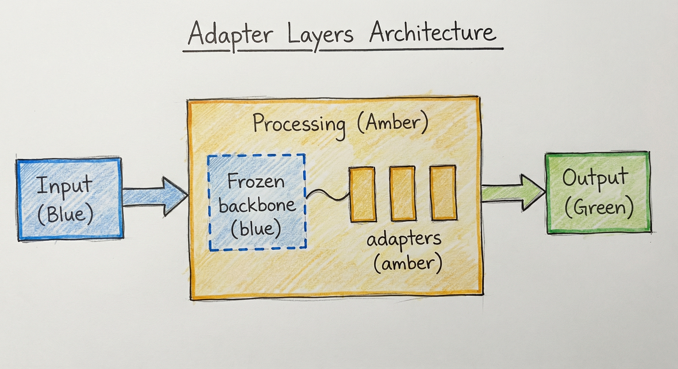
Adapter layers are small, trainable bottleneck modules inserted between the frozen layers of a pretrained transformer model, enabling parameter-efficient fine-tuning for downstream tasks. First proposed by Houlsby et al. in 2019, they were the pioneering PEFT method that proved you could adapt a massive model by training less than 4% of its parameters -- and lose almost nothing in quality.
The architecture is elegantly simple: each adapter is a two-layer feedforward network with a bottleneck. The input is projected down to a low dimension, passed through a non-linearity, and projected back up. A residual connection ensures the module can default to the identity function if the adaptation is unnecessary for that layer. Two adapters are typically inserted per transformer block -- one after the multi-head self-attention sublayer and one after the feed-forward network (FFN).
What makes adapter layers uniquely powerful compared to later PEFT methods like LoRA is their composability. Because adapters are separate modules (not weight modifications), you can stack, fuse, and swap them independently. The MAD-X framework demonstrated adapter-based cross-lingual transfer across 100+ languages. AdapterFusion showed how to combine task-specific adapters for multi-task learning without catastrophic forgetting. This modular philosophy -- train once, compose many ways -- is what keeps adapter layers relevant even in the age of LoRA.
For teams building multi-task, multi-lingual, or multi-domain systems where different capabilities need to be mixed and matched at serving time, adapter layers remain the gold standard for modular transfer learning.
Concept Snapshot
- What It Is
- Small bottleneck feedforward modules inserted between frozen transformer layers that learn task-specific representations while keeping the base model unchanged.
- Category
- Model Training
- Complexity
- Intermediate
- Inputs / Outputs
- Inputs: pretrained base model + task-specific training data + adapter config (bottleneck dimension, placement). Outputs: compact adapter weight files (per-task) that plug into the frozen base model at inference time.
- System Placement
- Sits in the fine-tuning stage of the ML pipeline, after pretraining and before model serving. Applied after data preparation and before evaluation/deployment. At inference time, adapters remain as separate modules inside the transformer (unlike LoRA, which merges away).
- Also Known As
- Bottleneck Adapters, Houlsby Adapters, Serial Adapters, Adapter Modules, Task Adapters
- Typical Users
- ML Engineers, NLP Engineers, Applied Scientists, Multilingual NLP Researchers, MLOps Engineers
- Prerequisites
- Transformer architecture (attention mechanism, feedforward layers), Transfer learning and fine-tuning fundamentals, Bottleneck / autoencoder concepts (dimensionality reduction), PyTorch or TensorFlow basics, GPU memory management basics
- Key Terms
- bottleneck dimensiondown-projectionup-projectionresidual connectionadapter fusionadapter compositionreduction factorfrozen weightsmodular transfer learning
Why This Concept Exists
The Multi-Task Fine-Tuning Problem
Before adapter layers, the standard approach to adapting a pretrained model like BERT to a downstream task was full fine-tuning: update every single parameter in the model for each new task. For a single task, this works great. But what happens when you have 26 tasks? Or 100 languages?
With BERT-Large (340M parameters), full fine-tuning creates a separate 1.3 GB model checkpoint per task. For an NLP platform supporting 26 tasks, that's 34 GB of model storage -- and each model must be loaded and served independently. For a company like Flipkart that needs sentiment analysis, intent classification, named entity recognition, and product categorization across 10+ Indian languages, the storage and serving costs become prohibitive.
Houlsby's Insight: Bottleneck Modules
In February 2019, Neil Houlsby and colleagues at Google published Parameter-Efficient Transfer Learning for NLP, introducing adapter modules. The key insight was that you don't need to modify the pretrained weights at all. Instead, you insert small trainable modules (adapters) at specific points within each transformer layer and train only those modules.
The adapter architecture borrows from the bottleneck concept in autoencoders: compress the representation into a lower dimension, apply a non-linearity, and decompress back. The bottleneck creates an information bottleneck that forces the adapter to learn only the most task-relevant transformations. A residual connection around the adapter ensures that if the adapter learns nothing useful, the layer's behavior is unchanged.
On the GLUE benchmark, adapters with only 3.6% additional parameters per task achieved performance within 0.4% of full fine-tuning. That's a 28x reduction in per-task storage with negligible quality loss.
From BERT to the Modular NLP Ecosystem
The real impact of adapters went beyond parameter efficiency. They introduced a modular paradigm for NLP:
-
AdapterHub (Pfeiffer et al., 2020) created a community repository of pretrained adapters that could be downloaded, composed, and shared -- like npm packages for NLP capabilities.
-
AdapterFusion (Pfeiffer et al., 2021) showed that multiple task adapters could be combined through learned attention weights, enabling multi-task knowledge transfer without catastrophic forgetting.
-
MAD-X (Pfeiffer et al., 2020) demonstrated cross-lingual transfer by stacking language adapters with task adapters, enabling zero-shot transfer to languages unseen during pretraining.
This modular ecosystem is why adapters remain relevant even after LoRA's rise. LoRA modifies weight matrices directly, making composition harder. Adapters are separate modules that can be stacked, swapped, and fused -- a property that's invaluable for complex multi-task or multi-lingual systems.
Key Takeaway: Adapter layers exist because full fine-tuning doesn't scale to multi-task, multi-lingual settings. They introduced the idea that task knowledge can be encapsulated in small, composable modules -- a paradigm that influenced all subsequent PEFT research.
Core Intuition & Mental Model
The Analogy: Universal Toolbox with Snap-On Attachments
Think of a pretrained transformer as a premium power drill. It's a general-purpose tool that works for many jobs. Full fine-tuning is like buying a completely separate drill for each job -- one for wood, one for metal, one for masonry. You end up with a garage full of expensive tools that are 95% identical.
Adapter layers are like snap-on drill bits. The drill (base model) stays the same. For each new material (task), you snap on a specialized bit (adapter) that handles the task-specific aspects. The bits are tiny compared to the drill itself, they're easy to swap, and you can even combine them -- a step bit for mixed materials, or a fusion of two bits for a specialized job.
The bottleneck design is key to this analogy: each adapter bit has a narrow shank (the bottleneck dimension) that focuses the adaptation on the most important aspects of the task. A wider shank gives more capacity but wastes material (parameters). A narrower shank is efficient but may not handle complex tasks.
The Information Bottleneck Intuition
Why does the bottleneck architecture work so well? Consider what happens during fine-tuning. Most of the knowledge a pretrained model has learned (syntax, semantics, world knowledge) is useful across tasks. Only a small amount of task-specific information needs to be added or modified.
The bottleneck forces the adapter to compress the layer's hidden representation through a narrow tube (say, 64 dimensions out of 768). Only the most task-relevant signal can pass through this bottleneck. Noise, task-irrelevant features, and redundant information are filtered out. The non-linearity (typically ReLU or GELU) adds the capacity to learn non-linear task-specific transformations that a simple linear projection couldn't capture.
The residual connection is the safety net: if the adapter can't improve on the pretrained representation for a given input, the residual path lets the original signal pass through unchanged. This means adapters can never make things worse -- they can only add task-specific value.
Why Composability Matters
Here's the intuition behind adapter composition. If you have a language adapter that knows Hindi syntax and a task adapter that knows sentiment classification (trained on English), you can stack them: the language adapter handles the linguistic adaptation, and the task adapter handles the task. Neither adapter needs to know about the other's job. This separation of concerns is what makes adapters uniquely powerful for multi-lingual, multi-task settings.
Mental Model: Adapters are like middleware in a software stack. Each adapter processes the data stream, applies its task-specific transformation, and passes the result along. The base model is the operating system -- general, powerful, and shared. The adapters are the apps -- specialized, lightweight, and composable.
Technical Foundations
The Bottleneck Adapter Architecture
Let be the hidden representation at a given point in a transformer layer, where is the model's hidden dimension (e.g., for BERT-Base, for Llama 7B).
An adapter module computes:
where:
- is the down-projection matrix
- is the up-projection matrix
- and are bias terms
- is a non-linear activation function (ReLU in the original paper, GELU in later work)
- is the bottleneck dimension, the only hyperparameter controlling capacity
- The leading term is the residual connection
Parameter Count Analysis
For a single adapter module:
For , this simplifies to approximately .
With two adapters per transformer layer (one after attention, one after FFN) across layers:
For BERT-Base (, ) with bottleneck :
BERT-Base has 110M parameters, so adapters add approximately 2.2% additional parameters per task.
For Llama 3 8B (, ) with bottleneck :
That's approximately 0.83% of the 8 billion base model parameters.
Reduction Factor
The AdapterHub library parameterizes the bottleneck dimension through a reduction factor :
Common reduction factors:
| Reduction Factor () | Bottleneck ( for ) | Adapter % (BERT-Base) | Typical Use Case |
|---|---|---|---|
| 2 | 384 | ~8.5% | Maximum capacity, complex tasks |
| 8 | 96 | ~2.1% | Strong default for NLU tasks |
| 16 | 48 | ~1.1% | Good balance of efficiency/quality |
| 64 | 12 | ~0.3% | Extreme compression, simple tasks |
Placement Variants
The original Houlsby configuration places adapters after both the attention and FFN sublayers. Pfeiffer et al. proposed a more efficient variant placing adapters only after the FFN sublayer, which halves the adapter parameter count with minimal quality loss. Formally:
Houlsby (two adapters per layer):
Pfeiffer (one adapter per layer, after FFN):
The Pfeiffer variant achieves comparable performance on most tasks while being more parameter-efficient.
Adapter Fusion Formulation
AdapterFusion learns to combine pretrained task adapters through an attention mechanism:
where the mixing weights are computed via a learned attention over adapter outputs:
Here , are learned query and key projections. This allows the model to dynamically weight different task adapters based on the current input, enabling non-destructive multi-task knowledge composition.
Practical Rule: Start with the Pfeiffer variant (one adapter after FFN) with reduction factor 16. If quality is insufficient, switch to the Houlsby variant (two adapters) and/or reduce the reduction factor to 8.
Internal Architecture
The adapter layer architecture inserts small bottleneck feedforward modules at specific points within each transformer block. In the standard Houlsby configuration, two adapter modules are placed per transformer layer: one immediately after the multi-head self-attention sublayer (post-attention adapter) and one immediately after the feed-forward network sublayer (post-FFN adapter). Each adapter consists of a down-projection, a non-linearity, an up-projection, and a residual connection.
The following diagram shows the placement of adapter modules within a single transformer block. The base transformer components (in gray) are frozen during training. Only the adapter modules (in green) and the layer normalization parameters (optionally) are updated.
The Pfeiffer variant simplifies this by placing only one adapter after the FFN sublayer, which halves the adapter parameter count. For LLM-scale models (7B+), the Pfeiffer placement is more common due to its better parameter-efficiency tradeoff. The parallel adapter variant, introduced in subsequent work, places the adapter in parallel with the FFN rather than serially, which can improve throughput at the cost of slightly different learning dynamics.
Key Components
Down-Projection Layer (W_down)
A linear layer that projects the hidden representation from the model dimension to the bottleneck dimension , where . This compression forces the adapter to learn only the most task-relevant transformations. Initialized with a small random distribution to break symmetry.
Non-Linearity
An activation function (ReLU in the original paper, GELU in modern implementations) applied after the down-projection. This is critical: without the non-linearity, the adapter would be equivalent to a single low-rank linear transformation (similar to LoRA). The non-linearity gives adapters strictly more representational power per parameter than LoRA.
Up-Projection Layer (W_up)
A linear layer that projects the bottleneck representation back to the model dimension . Together with , it forms the bottleneck structure. The combination of down-project, non-linearity, and up-project gives the adapter a two-layer MLP structure.
Residual Connection
Adds the original input to the adapter output, ensuring the adapter computes a modification to the representation rather than replacing it entirely. At initialization (with small random weights), the adapter output is near-zero, so the module approximately implements the identity function. This ensures training begins from the pretrained checkpoint's behavior.
Optional Layer Normalization
Some adapter configurations include a dedicated layer normalization within the adapter (before the down-projection or after the up-projection). This stabilizes training, especially for larger bottleneck dimensions. The AdapterHub library supports configuring layer norm placement via the original_ln_before and original_ln_after parameters.
Adapter Fusion Layer (optional)
When multiple task adapters are composed, an AdapterFusion layer learns attention weights over the outputs of different adapters. This enables the model to dynamically blend knowledge from multiple tasks based on the current input. The fusion parameters are trained in a separate stage after individual adapters are frozen.
Data Flow
Training Path: Input tokens pass through the frozen transformer layers. At each adapter-equipped layer, the hidden representation first flows through the frozen sublayer (attention or FFN), then through the trainable adapter module. The adapter compresses the representation through the bottleneck, applies a non-linearity, projects back up, and adds the residual. Only the adapter parameters (and optionally layer norm parameters) receive gradients -- the base model weights are completely frozen.
Inference Path: Identical to training but without gradient computation. Unlike LoRA, adapters are NOT merged into the base model. They remain as separate sequential modules, adding a small computational overhead for the two matrix multiplications per adapter per layer. For BERT-Base with bottleneck 64, this overhead is typically 5-8% of total inference time.
Multi-Adapter Composition: When multiple adapters are active (e.g., a language adapter + a task adapter in MAD-X), the data flows through each adapter sequentially within the same layer. The order of adapter application is determined by the composition configuration. In AdapterFusion mode, all adapter outputs are computed in parallel and then combined through a learned attention mechanism.
A flowchart showing a transformer block with frozen multi-head self-attention and feed-forward network components (gray), with two green trainable adapter modules inserted after each sublayer. An inset shows the adapter module detail: input flows through a down-projection to bottleneck dimension, through a non-linearity (orange), up-projection back to model dimension, and a residual addition with the original input.
How to Implement
Implementation Approaches
There are three primary ways to implement adapter layers in practice:
Approach 1: AdapterHub / HuggingFace Adapters Library -- The most feature-rich option for adapter-based PEFT. The adapters library (formerly adapter-transformers) provides Houlsby, Pfeiffer, and parallel adapter configurations, plus AdapterFusion and MAD-X composition out of the box. Best for BERT-family models and research.
Approach 2: HuggingFace PEFT -- The broader PEFT library supports bottleneck adapters alongside LoRA, prefix tuning, and other methods. It provides a unified API across model families but with fewer adapter-specific features than AdapterHub.
Approach 3: Custom Implementation -- For non-standard architectures or research, implementing adapter layers is straightforward: insert a nn.Module with down-projection, activation, up-projection, and residual at the appropriate points in the transformer. This gives full control over placement, initialization, and composition.
For production deployments, the key consideration is that adapters add sequential computation at inference time (unlike LoRA which merges away). This means adapter inference is slightly slower, but the tradeoff is full modularity -- you can swap, stack, and fuse adapters without reloading the base model.
Cost Note: Training adapters for a BERT-Base model on a classification task typically takes 1-2 hours on a single V100 GPU, costing approximately 12-20 (~INR 1,000-1,680). Full fine-tuning of the same 8B model would cost 4-8x more.
from transformers import AutoModelForSequenceClassification, AutoTokenizer, TrainingArguments, Trainer
from adapters import AutoAdapterModel, AdapterConfig
from datasets import load_dataset

# Load base model with adapter support
model_name = "bert-base-uncased"
model = AutoAdapterModel.from_pretrained(model_name)
tokenizer = AutoTokenizer.from_pretrained(model_name)

# Add a bottleneck adapter with Pfeiffer configuration
# Reduction factor 16 means bottleneck dimension = 768 / 16 = 48
adapter_config = AdapterConfig(
    mh_adapter=False,          # No adapter after attention (Pfeiffer variant)
    output_adapter=True,       # Adapter after FFN
    reduction_factor=16,       # Bottleneck dimension = d / 16
    non_linearity="relu",      # Activation function
)
model.add_adapter("sentiment", config=adapter_config)

# Add a classification head for the task
model.add_classification_head("sentiment", num_labels=2)

# Activate the adapter and freeze the base model
model.train_adapter("sentiment")

# Verify trainable parameters
total_params = sum(p.numel() for p in model.parameters())
trainable_params = sum(p.numel() for p in model.parameters() if p.requires_grad)
print(f"Trainable: {trainable_params:,} / {total_params:,} ({100*trainable_params/total_params:.2f}%)")
# Output: Trainable: ~900,000 / 110,000,000 (0.82%)

# Load and tokenize dataset
dataset = load_dataset("imdb")
def tokenize(batch):
    return tokenizer(batch["text"], padding="max_length", truncation=True, max_length=256)
tokenized = dataset.map(tokenize, batched=True)

# Train
training_args = TrainingArguments(
    output_dir="./adapter-sentiment",
    num_train_epochs=3,
    per_device_train_batch_size=32,
    learning_rate=1e-4,
    warmup_ratio=0.06,
    logging_steps=100,
    evaluation_strategy="epoch",
    save_strategy="epoch",
)

trainer = Trainer(
    model=model,
    args=training_args,
    train_dataset=tokenized["train"],
    eval_dataset=tokenized["test"],
    tokenizer=tokenizer,
)
trainer.train()

# Save only the adapter weights (~3.5 MB for BERT-Base)
model.save_adapter("./adapter-sentiment", "sentiment")
This example shows the standard workflow for training a bottleneck adapter using the AdapterHub adapters library. Key decisions:
- Pfeiffer variant (
mh_adapter=False, output_adapter=True): Only one adapter per layer (after FFN), halving the parameter count compared to the Houlsby variant. - reduction_factor=16: Bottleneck dimension of 48 for BERT-Base. This gives ~0.82% trainable parameters. Decrease to 8 for more capacity.
- Learning rate 1e-4: Higher than typical full fine-tuning rates (2e-5 to 5e-5) because adapters have far fewer parameters and benefit from larger steps.
- The saved adapter is only ~3.5 MB compared to the 440 MB full BERT-Base checkpoint.
from transformers import AutoTokenizer, TrainingArguments, Trainer
from adapters import AutoAdapterModel
from adapters.composition import Fuse

# Load model and add pretrained task adapters
model = AutoAdapterModel.from_pretrained("bert-base-uncased")
tokenizer = AutoTokenizer.from_pretrained("bert-base-uncased")

# Load three pretrained task adapters (e.g., from AdapterHub)
model.load_adapter("sentiment/sst-2@ukp", load_as="sst2")    # Sentiment
model.load_adapter("nli/multinli@ukp", load_as="mnli")        # NLI
model.load_adapter("sts/sts-b@ukp", load_as="stsb")           # Similarity

# Set up AdapterFusion to combine these adapters
# This adds lightweight fusion layers that learn to weight adapter outputs
adapter_setup = Fuse("sst2", "mnli", "stsb")
model.add_adapter_fusion(adapter_setup)
model.set_active_adapters(adapter_setup)

# Add a new classification head for the target task
model.add_classification_head("target_task", num_labels=3)

# Train ONLY the fusion layers (all adapters stay frozen)
model.train_adapter_fusion(adapter_setup)

# Verify: only fusion layers are trainable
trainable_params = sum(p.numel() for p in model.parameters() if p.requires_grad)
print(f"Fusion trainable params: {trainable_params:,}")
# Output: ~300,000 fusion parameters

# Standard HuggingFace training loop
training_args = TrainingArguments(
    output_dir="./adapter-fusion-output",
    num_train_epochs=5,
    per_device_train_batch_size=32,
    learning_rate=5e-5,
    evaluation_strategy="epoch",
)

# ... train with Trainer as usual
# The fusion layers learn which adapter to weight more for each input
# model.save_adapter_fusion("./fusion-weights", "sst2,mnli,stsb")
AdapterFusion is the killer feature of adapter layers that has no direct equivalent in LoRA. The process works in two stages:
- Stage 1 (Knowledge Extraction): Train individual adapters on separate tasks. Each adapter encapsulates task-specific knowledge.
- Stage 2 (Knowledge Composition): Freeze all adapters and train lightweight fusion layers that learn to combine adapter outputs via attention.
The fusion layers learn input-dependent mixing weights: for some inputs, the sentiment adapter is most useful; for others, the NLI adapter contributes more. This is non-destructive -- no adapter is modified, and new adapters can be added to the fusion later.
import torch
import torch.nn as nn


class BottleneckAdapter(nn.Module):
    """A single bottleneck adapter module."""

    def __init__(
        self,
        hidden_dim: int,
        bottleneck_dim: int,
        activation: str = "relu",
        init_scale: float = 1e-3,
    ):
        super().__init__()
        self.down_proj = nn.Linear(hidden_dim, bottleneck_dim)
        self.up_proj = nn.Linear(bottleneck_dim, hidden_dim)

        # Activation function
        if activation == "relu":
            self.activation = nn.ReLU()
        elif activation == "gelu":
            self.activation = nn.GELU()
        else:
            raise ValueError(f"Unsupported activation: {activation}")

        # Initialize with small weights for near-identity at start
        nn.init.normal_(self.down_proj.weight, std=init_scale)
        nn.init.zeros_(self.down_proj.bias)
        nn.init.normal_(self.up_proj.weight, std=init_scale)
        nn.init.zeros_(self.up_proj.bias)

    def forward(self, x: torch.Tensor) -> torch.Tensor:
        # Residual connection: adapter output is ADDED to input
        residual = x
        x = self.down_proj(x)         # (batch, seq, hidden) -> (batch, seq, bottleneck)
        x = self.activation(x)        # Non-linear transformation
        x = self.up_proj(x)           # (batch, seq, bottleneck) -> (batch, seq, hidden)
        return residual + x           # Residual connection


def inject_adapters(
    model: nn.Module,
    bottleneck_dim: int = 64,
    placement: str = "pfeiffer",  # "houlsby" or "pfeiffer"
) -> nn.Module:
    """Inject bottleneck adapters into a transformer model.

    This function freezes all base model parameters and inserts
    trainable adapter modules at the appropriate locations.
    """
    # Step 1: Freeze all base model parameters
    for param in model.parameters():
        param.requires_grad = False

    # Step 2: Insert adapters into each transformer layer
    for layer in model.transformer.layers:  # Adjust attribute path for your model
        hidden_dim = layer.self_attn.out_proj.out_features

        if placement in ("houlsby", "both"):
            # Adapter after self-attention
            layer.post_attn_adapter = BottleneckAdapter(hidden_dim, bottleneck_dim)

        # Adapter after FFN (both Houlsby and Pfeiffer)
        layer.post_ffn_adapter = BottleneckAdapter(hidden_dim, bottleneck_dim)

    # Step 3: Modify the forward pass to route through adapters
    # (In practice, you'd subclass or monkey-patch the layer's forward method)

    trainable = sum(p.numel() for p in model.parameters() if p.requires_grad)
    total = sum(p.numel() for p in model.parameters())
    print(f"Injected adapters: {trainable:,} trainable / {total:,} total ({100*trainable/total:.2f}%)")

    return model


# Usage example
# model = AutoModelForCausalLM.from_pretrained("meta-llama/Llama-3.1-8B")
# model = inject_adapters(model, bottleneck_dim=128, placement="pfeiffer")
# Output: Injected adapters: ~33,600,000 trainable / 8,000,000,000 total (0.42%)
This from-scratch implementation demonstrates the core adapter mechanics. Key implementation details:
- Small initialization (
init_scale=1e-3): The adapter output starts near-zero, so the residual connection dominates. The model begins from the pretrained behavior and gradually learns task-specific modifications. - Residual connection: The
return residual + xensures the adapter can only modify the representation, not replace it. This is the architectural guarantee that adapters start from a good initialization. - Placement choice: The
pfeiffervariant inserts one adapter per layer (after FFN);houlsbyinserts two (after attention and after FFN). Pfeiffer uses half the parameters with comparable quality on most tasks.
For production use, prefer the AdapterHub library which handles serialization, composition, and the many edge cases around different model architectures.
from adapters import AutoAdapterModel
from adapters.composition import Stack

# Load multilingual base model
model = AutoAdapterModel.from_pretrained("xlm-roberta-base")

# Step 1: Load a language adapter (trained on Hindi unlabeled text)
model.load_adapter("hi/wiki@ukp", load_as="hindi_lang")

# Step 2: Load a task adapter (trained on English NER data)
model.load_adapter("ner/conll2003@ukp", load_as="english_ner")

# Step 3: Stack language adapter BELOW task adapter
# Data flows: input -> hindi_lang adapter -> english_ner adapter -> output
model.set_active_adapters(Stack("hindi_lang", "english_ner"))

# Now the model performs Hindi NER despite the NER adapter
# being trained only on English data!
# The language adapter handles linguistic adaptation,
# the task adapter handles task-specific processing.

# For inference on Hindi text:
from transformers import AutoTokenizer
import torch

tokenizer = AutoTokenizer.from_pretrained("xlm-roberta-base")
text = "नरेंद्र मोदी ने नई दिल्ली में G20 शिखर सम्मेलन की मेजबानी की"
inputs = tokenizer(text, return_tensors="pt")

with torch.no_grad():
    outputs = model(**inputs)
    # outputs contain NER predictions for Hindi text
    predictions = torch.argmax(outputs.logits, dim=-1)
    print(predictions)
This example demonstrates the MAD-X framework for zero-shot cross-lingual transfer. The key idea is separation of concerns through adapter stacking:
- Language adapter (
hindi_lang): Trained on unlabeled Hindi text using masked language modeling. It learns Hindi-specific linguistic patterns and adapts the multilingual model's representations to Hindi. - Task adapter (
english_ner): Trained on English NER data. It learns the task-specific patterns for named entity recognition.
When stacked, the language adapter first transforms the representation into a language-normalized space, and the task adapter then applies NER-specific processing. This enables zero-shot transfer to languages with no task-specific training data -- crucial for low-resource Indian languages like Bhojpuri, Maithili, or Dogri where labeled NER data is scarce.
# Adapter configuration (YAML format for reference)
model:
  name: bert-base-uncased
  # or: meta-llama/Llama-3.1-8B

adapter:
  # Adapter variant: "houlsby" (2 per layer) or "pfeiffer" (1 per layer)
  variant: pfeiffer
  reduction_factor: 16        # bottleneck_dim = hidden_dim / 16
  non_linearity: relu          # relu, gelu, swish
  # If using Houlsby:
  # mh_adapter: true           # Adapter after attention
  # output_adapter: true       # Adapter after FFN

  # Layer normalization (optional)
  original_ln_before: true
  original_ln_after: true

  # Composition (optional)
  composition: null             # null, stack, fuse
  # For MAD-X stacking:
  # composition: stack
  # language_adapter: hi/wiki@ukp
  # task_adapter: ner/conll2003@ukp

training:
  epochs: 5
  batch_size: 32
  learning_rate: 1e-4
  warmup_ratio: 0.06
  lr_scheduler: linear
  max_seq_length: 256
  weight_decay: 0.01

serving:
  # Adapters stay as separate modules (no merging)
  multi_adapter: false
  adapter_cache_size: 32       # Max adapters cached in GPU memory
Common Implementation Mistakes
- ●
Using too small a bottleneck dimension: With reduction factor 64 or higher, the adapter has very few parameters and may not capture sufficient task-specific information. For complex tasks like reading comprehension or multi-label classification, use reduction factor 8-16. A good diagnostic: if the adapter-tuned model barely beats the frozen base model, the bottleneck is too narrow.
- ●
Forgetting to freeze base model parameters: If you accidentally leave base model parameters trainable alongside adapters, you get a confusing hybrid where both are updating. This defeats the purpose of adapters (parameter isolation) and can cause training instability. Always call
model.train_adapter(adapter_name)or manually setparam.requires_grad = Falsefor base parameters. - ●
Ignoring the inference latency overhead: Unlike LoRA (which merges away), adapter layers remain as separate sequential modules during inference. Each adapter adds two matrix multiplications per layer. For latency-sensitive applications, benchmark the overhead carefully. For BERT-Base with 12 layers and 2 adapters each, expect 5-8% latency increase.
- ●
Training fusion layers before individual adapters are good: AdapterFusion combines the outputs of pretrained adapters. If the individual adapters are poorly trained or irrelevant to the target task, fusion cannot compensate. Always validate individual adapter quality before attempting fusion.
- ●
Applying LoRA conventions to adapter hyperparameters: Adapter learning rates are typically higher (1e-4 to 5e-4) than full fine-tuning but follow different dynamics than LoRA. Using LoRA's recommended learning rates (2e-4 with alpha scaling) without understanding adapter-specific behavior can lead to suboptimal results.
- ●
Not leveraging the residual connection during debugging: The residual connection means that at initialization, the adapter is approximately an identity function. If training shows no improvement, the adapter may be stuck at identity. Check that gradients are flowing through the adapter (not just the residual path) by monitoring gradient norms on the down/up projection weights.
When Should You Use This?
Use When
You need modular, composable task capabilities that can be mixed and matched at serving time -- adapter layers are the only PEFT method with a mature composition framework (AdapterFusion, Stack, Split)
You're building a multi-lingual NLP system and need zero-shot cross-lingual transfer via the MAD-X paradigm -- stacking language adapters with task adapters enables transfer to 100+ languages
Your organization has a shared model platform where different teams add task-specific capabilities to a common base model without coordinating with each other -- adapters are independent modules that don't interfere
You need to preserve the exact base model weights at all times (e.g., for regulatory compliance or reproducibility) -- adapters never modify the base model, unlike LoRA which merges into it
You want to reuse task knowledge from previously trained adapters for new tasks via AdapterFusion -- this is particularly valuable when you have a library of existing task adapters
You're working with BERT-family encoder models for NLU tasks (classification, NER, QA) where the AdapterHub ecosystem provides a rich library of pretrained adapters
Your fine-tuning dataset is small to medium (1K-50K examples) and you need the implicit regularization from the bottleneck architecture to prevent overfitting
Avoid When
Inference latency is critical and you cannot tolerate even 5-8% additional overhead -- LoRA's merge-and-deploy approach has zero latency penalty, while adapters remain as sequential computation
You need to fine-tune a very large model (70B+) and memory is the primary constraint -- LoRA and QLoRA are more memory-efficient than adapters for the same number of trainable parameters because adapters also store intermediate activations for the adapter modules
You're doing simple single-task fine-tuning with no plans for multi-task composition -- LoRA is simpler, has better tooling for modern LLMs, and produces smaller checkpoints
You're working with a decoder-only LLM (GPT, Llama) for text generation and don't need multi-task composition -- LoRA has better empirical results and ecosystem support for autoregressive generation tasks
Your deployment platform requires merged model weights (e.g., some edge deployment frameworks can't handle dynamic module insertion) -- adapters cannot be merged like LoRA
You need the absolute best quality and have unlimited compute -- full fine-tuning still holds a slight edge for complex tasks with large datasets
Key Tradeoffs
The Core Tradeoff: Modularity vs. Inference Efficiency
Adapter layers sit at a unique point in the PEFT design space: they provide the best composability of any PEFT method at the cost of additional inference computation. This is the inverse of LoRA's tradeoff (best inference efficiency, but limited composability).
| Property | Adapter Layers | LoRA | Prefix Tuning | Full Fine-tuning |
|---|---|---|---|---|
| Inference overhead | 5-8% latency | 0% (after merge) | 0-3% (context reduction) | 0% |
| Composability | Excellent (Fusion, Stack) | Limited (arithmetic only) | Poor | None |
| Params per task (BERT-Base) | 0.5-3.6% | 0.1-0.5% | 0.1% | 100% |
| Multi-lingual transfer | MAD-X (excellent) | Basic (per-language adapters) | Limited | Per-language model |
| Ecosystem maturity | AdapterHub (encoders) | PEFT/vLLM (decoders) | Limited | Universal |
When Modularity Wins
Consider a company like an Indian e-commerce platform that needs:
- Sentiment analysis in Hindi, Tamil, Telugu, Bengali
- Product categorization across 10 categories
- Intent classification for customer support
- Named entity recognition for address parsing
With adapters: one XLM-RoBERTa base model + 4 language adapters + 4 task adapters = 8 tiny adapter files. Total storage: ~30 MB of adapters on top of the 1.1 GB base model. Any combination of language + task works through stacking.
With LoRA: you'd need 4 x 4 = 16 separate LoRA adapters (one per language-task pair), or complex multi-task training to capture all combinations. Total storage may be similar, but the combinatorial explosion in training is painful.
Cost Comparison for Adapter Training
| Model | Hardware | Time (50K examples) | Cloud Cost | Cost (INR) |
|---|---|---|---|---|
| BERT-Base (adapter) | 1x V100 16GB | ~2 hrs | ~$6 | ~INR 500 |
| BERT-Large (adapter) | 1x A10G 24GB | ~4 hrs | ~$8 | ~INR 670 |
| Llama 3 8B (adapter) | 1x A100 80GB | ~5 hrs | ~$20 | ~INR 1,680 |
| Llama 3 8B (LoRA r=16) | 1x A100 80GB | ~4 hrs | ~$16 | ~INR 1,340 |
| Llama 3 8B (full FT) | 4x A100 80GB | ~8 hrs | ~$128 | ~INR 10,750 |
Practitioner's Note: If you're building a single-task system with a decoder-only LLM, use LoRA. If you're building a multi-task or multi-lingual platform on encoder models, adapters with AdapterFusion are the stronger choice. The decision is about your deployment topology, not about raw performance numbers.
Alternatives & Comparisons
LoRA modifies weight matrices directly through low-rank decomposition, enabling zero-overhead inference after merging. It's more parameter-efficient per trainable parameter and has better ecosystem support for modern decoder-only LLMs. Choose LoRA for single-task fine-tuning, latency-sensitive applications, and LLM-scale models. Choose adapters when you need modularity, composition (AdapterFusion), or multi-lingual transfer (MAD-X).
QLoRA combines 4-bit quantization with LoRA, enabling fine-tuning of very large models on limited hardware. It's strictly more memory-efficient than adapter layers but lacks the composability features. Choose QLoRA when GPU memory is the binding constraint and you need single-task adaptation. Choose adapters when you need multi-task composition capabilities.
Prefix tuning prepends learnable continuous vectors to attention keys and values at each layer. It's more parameter-efficient than adapters but consumes part of the context window and underperforms on complex tasks. Choose prefix tuning for lightweight, low-complexity tasks. Choose adapters for better quality and composability.
Prompt tuning learns soft prompt embeddings at the input layer only. It uses the fewest parameters of any PEFT method but has the weakest performance, especially on smaller models. Choose prompt tuning for simple classification with very large models (100B+). Choose adapters for broader task coverage and better quality on medium-sized models.
IA3 learns rescaling vectors (not matrices) applied to key, value, and FFN activations. It trains even fewer parameters than adapters but lacks the non-linearity that gives adapters their expressiveness. Choose IA3 for extremely parameter-constrained scenarios. Choose adapters when you need more expressive task-specific transformations.
Full fine-tuning updates all model parameters, achieving the best possible quality but at enormous compute and storage costs. Each task requires a full model copy. Choose full fine-tuning only when you have abundant compute, large datasets, and need maximum quality for a single critical task. Choose adapters for everything else, especially multi-task scenarios.
Pros, Cons & Tradeoffs
Advantages
Best-in-class composability: Adapters are the only PEFT method with a mature composition framework. AdapterFusion, Stack, and Split enable combining task-specific, language-specific, and domain-specific adapters in arbitrary configurations -- impossible with LoRA or prefix tuning.
Excellent multi-lingual transfer: The MAD-X framework enables zero-shot cross-lingual transfer by stacking language and task adapters. This is critical for supporting low-resource Indian languages (Maithili, Dogri, Bhojpuri) where labeled task data doesn't exist.
Base model integrity preserved: Adapters never modify the pretrained weights. The base model remains bit-for-bit identical regardless of how many adapters are trained. This simplifies model management, compliance, and debugging compared to LoRA's weight merging.
Non-linear expressiveness: Unlike LoRA (which is a linear low-rank update), adapters include a non-linearity between the down and up projections. This gives them strictly more representational power per parameter for learning complex task-specific transformations.
Rich pretrained adapter ecosystem: AdapterHub hosts hundreds of pretrained adapters for tasks, languages, and domains that can be downloaded and composed without any training. This is like an app store for model capabilities.
Clean separation of concerns: Each adapter encapsulates exactly one capability (task, language, or domain). This makes it easy to debug, version, and A/B test individual capabilities without affecting others.
Strong regularization through bottleneck: The bottleneck architecture naturally limits the adapter's capacity, providing implicit regularization that prevents overfitting on small datasets. Reduction factor 16 is typically sufficient for datasets as small as 1K examples.
Disadvantages
Inference latency overhead: Adapters add sequential computation at inference time (two matrix multiplications per adapter per layer). For BERT-Base, this is 5-8% overhead; for a Llama 8B model with adapters in all 32 layers, it can reach 10-15%. This overhead is permanent and cannot be eliminated by merging.
Less parameter-efficient than LoRA: For the same quality on single-task benchmarks, adapters typically use 2-5x more parameters than LoRA. A BERT-Base adapter at reduction factor 16 uses ~0.8% of parameters; LoRA at rank 8 achieves similar quality with ~0.2%.
Weaker ecosystem support for modern LLMs: The AdapterHub ecosystem was built primarily for BERT-family encoder models. While the
adapterslibrary now supports decoder models, LoRA has much better tooling for Llama, Mistral, and other modern LLMs through PEFT, Unsloth, and Axolotl.Cannot merge into base model: After training, adapters remain as separate modules. You can't fold them into the base weights like LoRA. This means every adapter-equipped model must carry the adapter overhead at inference time, and deployment requires adapter-aware serving infrastructure.
Activation memory overhead during training: Adapter modules introduce additional intermediate activations that must be stored for backpropagation. For each adapter, the bottleneck activations add memory per layer, where is batch size and is sequence length.
Complexity of multi-adapter serving: While adapter composition is powerful in theory, serving multiple stacked or fused adapters adds engineering complexity. Request routing must track which adapter combination each request needs, and adapter caching strategies are needed to avoid repeated loading from disk.
Failure Modes & Debugging
Bottleneck Dimension Too Narrow
Cause
Using an excessively high reduction factor (e.g., 64 or 128) that compresses the representation to a dimension too small to capture task-specific information. This is analogous to using too low a rank in LoRA, but the effect is more severe because the non-linearity amplifies information loss at very small dimensions.
Symptoms
Training loss decreases slowly and plateaus far above the full fine-tuning baseline. The adapter-tuned model shows marginal improvement over the frozen base model (often <2% accuracy gain). Per-layer gradient analysis shows very small gradients in the up-projection, indicating the bottleneck is destroying useful signal.
Mitigation
Start with reduction factor 16 (bottleneck = d/16) and decrease to 8 or 4 if quality is insufficient. As a diagnostic, train with reduction factor 2 (50% of model dimension) to establish an upper bound. If the gap between RF=16 and RF=2 is large (>3%), the task requires more adapter capacity. Consider switching to the Houlsby variant (two adapters per layer) for additional capacity without widening the bottleneck.
Adapter Stacking Order Mismatch in MAD-X
Cause
In cross-lingual transfer with MAD-X, placing the task adapter below the language adapter (or omitting the language adapter entirely). The correct order is language adapter first (bottom), then task adapter (top). Reversing this means the task adapter receives non-language-adapted representations, producing incorrect predictions.
Symptoms
Cross-lingual transfer performance is significantly worse than expected -- often worse than using just the task adapter alone. The model may produce outputs biased toward the source language (e.g., English-like structures when processing Hindi text). The language adapter's contribution is effectively bypassed.
Mitigation
Always stack in the order Stack(language_adapter, task_adapter) where the language adapter processes the input first. Validate the stacking order by comparing performance to a baseline without language adapters -- the stacked configuration should always improve. Use the AdapterHub documentation's composition examples as reference templates.
Catastrophic Forgetting During Sequential Adapter Training
Cause
Training multiple adapters sequentially on the same base model instance without proper isolation. If adapter A is trained and then adapter B is trained on the same model object, the shared layer norm parameters (which are often unfrozen) may be corrupted for adapter A.
Symptoms
The first adapter's performance degrades after training the second adapter. Evaluating adapter A after training adapter B shows decreased accuracy. The issue is subtle because the adapter weights themselves are correct -- it's the shared layer norm parameters that have shifted.
Mitigation
Always start from a fresh base model checkpoint when training a new adapter, or ensure that layer norm parameters are frozen during adapter training. The AdapterHub library handles this correctly when using model.train_adapter(), but custom implementations must be careful to freeze layer norms or save/restore them between adapter training runs.
AdapterFusion Underfitting Due to Irrelevant Source Adapters
Cause
Including adapters in a fusion setup that are unrelated to the target task. The fusion attention mechanism wastes capacity learning to suppress irrelevant adapters instead of leveraging useful ones. With too many irrelevant adapters, the fusion layer may struggle to identify the useful signal.
Symptoms
Fusion performance is worse than the best individual adapter alone. The learned fusion weights show near-uniform distribution across adapters (no clear winner), or the fusion assigns high weight to an irrelevant adapter due to spurious correlations in the training data.
Mitigation
Curate the adapter set for fusion carefully. Include only adapters whose tasks are related to the target. Start with 2-3 adapters and add more incrementally, measuring whether each addition improves fusion performance. Monitor the learned fusion weights to verify they are meaningful (not uniform or degenerate).
Inference Latency Accumulation with Multiple Stacked Adapters
Cause
Stacking three or more adapters (e.g., language adapter + domain adapter + task adapter) introduces cumulative sequential computation. Each adapter adds 5-8% latency per layer, and stacking three adapters can increase total inference time by 15-25%.
Symptoms
Inference latency exceeds SLA requirements. P99 latency shows high variance because adapter computation adds to the critical path. In production, request timeouts increase, especially for longer sequences where the per-token overhead accumulates across many decoding steps.
Mitigation
Use AdapterDrop to remove adapters from lower transformer layers where they contribute less (Ruckle et al. showed removing adapters from the first 5 layers preserves most quality while cutting adapter inference cost by 39%). For latency-critical systems, consider training a single combined adapter instead of stacking multiple ones, sacrificing modularity for speed.
GPU Memory Fragmentation from Dynamic Adapter Loading
Cause
In multi-tenant serving where adapters are loaded and unloaded dynamically per request, GPU memory becomes fragmented. Different adapters have slightly different memory footprints depending on bottleneck dimensions, and frequent allocation/deallocation creates unusable memory gaps.
Symptoms
GPU memory utilization appears high but actual usable memory is low. New adapter loading fails with OOM errors despite sufficient total free memory. Serving throughput degrades over time as fragmentation accumulates. The issue is particularly severe with CUDA's default memory allocator.
Mitigation
Pre-allocate a fixed-size adapter memory pool on the GPU and assign adapter slots from this pool. Use a LRU (Least Recently Used) cache to manage which adapters are resident in GPU memory. Set all adapters to use the same bottleneck dimension to ensure uniform memory allocation sizes. Consider using PyTorch's CUDA memory allocator with expandable_segments enabled for better fragmentation handling.
Placement in an ML System
Where Adapters Fit in the ML System
Adapter layers occupy the adaptation and composition stage in an ML pipeline, sitting between base model pretraining and production serving. The typical workflow involves multiple phases:
- Base model selection: Choose a pretrained transformer from a model hub (BERT for NLU tasks, XLM-RoBERTa for multilingual, Llama for generation).
- Language adapter training (optional, for multilingual): Train language-specific adapters on unlabeled text using masked language modeling.
- Task adapter training: Train task-specific adapters on labeled task data with the base model frozen.
- Adapter composition (optional): Use AdapterFusion to combine task adapters, or Stack to combine language + task adapters.
- Evaluation: Benchmark individual and composed adapter configurations on held-out test sets.
- Deployment: Load the base model once and serve adapters dynamically per request.
In an Indian enterprise context, consider a company like Razorpay building a fraud detection platform across multiple transaction types. A single XLM-RoBERTa model serves as the base, with task adapters for UPI fraud, credit card fraud, and account takeover detection, plus language adapters for processing merchant descriptions in Hindi, English, and regional languages. The adapter composition layer decides which adapters to activate based on the transaction type and language.
Organizational Pattern: In large ML platforms, adapters enable a hub-and-spoke model. The central ML team maintains the base model and serving infrastructure. Individual product teams train and deploy their own adapters without coordinating with the central team or each other. This decentralized approach to model customization is particularly valuable for organizations with many teams and diverse NLP needs.
Pipeline Stage
Training / Fine-tuning
Upstream
- Data Preprocessing Pipeline (cleaned, formatted training data per task)
- Base Model Selection (pretrained checkpoint -- BERT, XLM-RoBERTa, Llama)
- Tokenizer Configuration
- Language Adapter Training (for MAD-X cross-lingual setups)
Downstream
- Adapter Storage / Model Registry (versioned adapter checkpoints)
- Adapter Composition Layer (fusion, stacking configuration)
- Model Serving (adapter-aware inference engine)
- Model Evaluation & Benchmarking
Scaling Bottlenecks
During training, the bottleneck is the same as any fine-tuning: activation memory from the full forward pass through the base model. Adapters add modest additional activation memory (the bottleneck activations at each layer), but this is typically <5% overhead compared to the base model's activations.
At inference time, the scaling bottleneck is fundamentally different from LoRA. Because adapters are sequential modules that cannot be merged, every inference request must pass through the adapter computation. For a single adapter, the overhead is manageable (5-8%). But in multi-adapter stacking (e.g., MAD-X with 2-3 adapters per layer), the overhead compounds to 15-25%, which can become the dominant bottleneck for latency-sensitive applications.
Multi-tenant serving faces an adapter management bottleneck. Each adapter set must be resident in GPU memory for the requests that need it. With hundreds of adapter combinations (languages x tasks), the adapter cache management becomes a scheduling problem. AdapterDrop helps by removing adapters from lower layers, but the fundamental tension between adapter diversity and GPU memory capacity remains.
For distributed inference (tensor parallelism or pipeline parallelism), adapter layers must be correctly partitioned across devices. This is more complex than distributing base model weights because adapter composition logic must be preserved. The AdapterHub library doesn't yet support tensor-parallel adapter serving, which limits adapters to single-GPU inference for most deployments.
Production Case Studies
Google Research authored the original adapter layers paper (Houlsby et al., 2019) and demonstrated the technique on BERT. They showed that inserting tiny bottleneck modules between transformer layers could match full fine-tuning performance while adding only 3.6% parameters per task. They also released the adapter-bert reference implementation on GitHub, which became the foundation for the AdapterHub ecosystem.
Adapters achieved within 0.4% of full fine-tuning performance on the GLUE benchmark while requiring only 3.6% additional parameters per task. On 26 diverse text classification tasks, adapters matched or exceeded full fine-tuning on the majority of tasks. The adapter checkpoint per task was ~13 MB vs. ~440 MB for a full BERT-Base checkpoint -- a 34x storage reduction.
The UKP Lab at TU Darmstadt, led by Jonas Pfeiffer and colleagues, created AdapterHub -- a community platform and library for sharing and composing pretrained adapters. They also introduced AdapterFusion (non-destructive multi-task composition) and MAD-X (cross-lingual adapter stacking), establishing the theoretical and practical foundations for modular transfer learning in NLP.
AdapterHub grew to host hundreds of pretrained adapters across tasks, languages, and domains. AdapterFusion demonstrated that composing pretrained adapters outperformed both individual adapters and multi-task fine-tuning on 16 diverse NLU tasks. The adapters library (formerly adapter-transformers) has been downloaded over 1 million times from PyPI.
Bapna and Firat at Google applied adapter layers to massively multilingual machine translation covering 103 languages. They injected lightweight adapters into a shared multilingual NMT model, allowing each language pair to have its own adapter while sharing the massive base model. This approach bridged the quality gap between individual bilingual models and a single massively multilingual model.
Language-pair-specific adapters (with only a small fraction of the base model's parameters) closed the quality gap between individual bilingual models and the shared multilingual model for most of the 103 language pairs. The approach enabled scalable multilingual MT without the prohibitive cost of training and serving 103 separate bilingual models.
AI4Bharat, the initiative at IIT Madras, has leveraged adapter-based and PEFT approaches for building NLP capabilities across 22 scheduled Indian languages. Their work on IndicBERT, IndicBART, and IndicTrans2 includes adapter-style fine-tuning for low-resource languages where full fine-tuning data is scarce. The adapter paradigm is particularly valuable for languages like Maithili, Santali, and Dogri where labeled task data is extremely limited.
AI4Bharat's multilingual models and adapter-based approaches have enabled NLP capabilities for Indian languages that were previously underserved. IndicTrans2 supports translation across all 22 scheduled languages, and the PEFT approach keeps compute costs manageable for the research lab context -- critical since Indian academic GPU budgets are a fraction of those at US tech companies.
Tooling & Ecosystem
The most comprehensive adapter library, providing Houlsby, Pfeiffer, and parallel adapter configurations, plus AdapterFusion, MAD-X stacking, AdapterDrop, and IA3. Built on top of Hugging Face Transformers with full compatibility. Supports composition blocks (Fuse, Stack, Split, BatchSplit) for complex multi-adapter setups. Now supports decoder models alongside the original encoder focus.
Community platform hosting hundreds of pretrained adapters for tasks, languages, and domains. Adapters can be downloaded with a single line of code and composed through the adapters library. Includes adapters for NLU tasks (sentiment, NLI, QA), languages (100+ via MAD-X), and domains. Functions as the 'npm for NLP adapters'.
The broader PEFT library supports bottleneck adapters alongside LoRA, QLoRA, prefix tuning, and other methods via a unified API. While it has fewer adapter-specific features than the dedicated adapters library (no AdapterFusion), it provides better coverage of modern LLM architectures (Llama, Mistral, Gemma) and integrates with TRL for RLHF/DPO training.
A framework specifically designed for applying adapter-based PEFT to large language models (LLaMA, BLOOM, GPT-J). Supports series adapters, parallel adapters, and LoRA with systematic benchmarking of placement strategies. Published at EMNLP 2023 with comprehensive experiments on reasoning tasks showing 7B adapter-tuned models competitive with 175B zero-shot models.
The original reference implementation of adapter layers for BERT from Houlsby et al. (2019). Based on TensorFlow and the official BERT codebase. While not actively maintained, it serves as the canonical reference for the Houlsby adapter architecture and initialization strategy.
Research & References
Houlsby, Giurgiu, Jastrzebski, Morrone, de Laroussilhe, Gesmundo, Attariyan & Gelly (2019)ICML 2019
The foundational adapter layers paper. Introduced bottleneck adapter modules inserted between transformer layers, achieving within 0.4% of full fine-tuning performance on GLUE while adding only 3.6% parameters per task. Established the adapter architecture (down-projection, non-linearity, up-projection, residual) that all subsequent work builds upon.
Pfeiffer, Kamath, Ruckle, Cho & Gurevych (2021)EACL 2021
Proposed a two-stage learning algorithm: first train individual task adapters, then learn fusion layers that combine adapter outputs via attention. This non-destructive approach outperformed multi-task fine-tuning and individual adapters on 16 NLU tasks, demonstrating that adapter composition is more effective than training a single multi-task model.
Pfeiffer, Vulic, Gurevych & Ruder (2020)EMNLP 2020
Introduced the MAD-X framework for cross-lingual transfer by stacking language adapters with task adapters. Included a novel invertible adapter architecture. Outperformed state-of-the-art on cross-lingual NER and commonsense reasoning across typologically diverse languages, enabling zero-shot transfer to languages unseen during pretraining.
Pfeiffer, Ruckle, Poth, Kamath, Mulling, Schimpf, Schulz, Borber, Geigle, Glockner, Gurevych & Vulic (2020)EMNLP 2020 (System Demonstration)
Introduced AdapterHub, a community platform and library for sharing and composing pretrained adapters. Built on Hugging Face Transformers, it enables dynamic stitching-in of pretrained adapters for different tasks and languages. Established the adapter sharing paradigm that makes modular transfer learning practical.
Ruckle, Geigle, Glockner, Beck, Pfeiffer, Reimers & Gurevych (2021)EMNLP 2021
Proposed removing adapter modules from lower transformer layers during training and inference. Showed that dropping adapters from the first 5 layers preserved most task performance while making inference 39% faster when running 8 tasks simultaneously. Also demonstrated that adapter weights can be shared across layers with minimal quality loss.
He, Zhou, Ma, Berg-Kirkpatrick & Neubig (2022)ICLR 2022 (Spotlight)
Established a unified theoretical framework connecting adapters, prefix tuning, and LoRA. Showed that all PEFT methods can be viewed as modifications to specific hidden states, varying along dimensions like modification function and application position. Proposed the MAM (Mix-And-Match) Adapter that combines insights from multiple PEFT approaches.
Hu, Huang, Shi, Liu, Zhang, Wang, Chen, Xia, Yu, Li & Chen (2023)EMNLP 2023
Systematically evaluated adapter placement strategies (serial, parallel) for modern LLMs (LLaMA, BLOOM, GPT-J). Found that series adapters work best after MLP layers, while parallel adapters work best alongside MLP layers. Demonstrated that 7B adapter-tuned models can match 175B zero-shot models on math and reasoning benchmarks.
Bapna & Firat (2019)EMNLP 2019
Applied adapter layers to massively multilingual NMT covering 103 languages. Demonstrated that lightweight per-language-pair adapters injected into a shared multilingual model can bridge the quality gap to individual bilingual models, paving the way toward universal machine translation with parameter-efficient adaptation.
Interview & Evaluation Perspective
Common Interview Questions
- ●
Explain how adapter layers work. What is the bottleneck architecture and why is it effective?
- ●
Compare adapter layers with LoRA -- when would you choose one over the other?
- ●
How does AdapterFusion work? Why is non-destructive task composition valuable?
- ●
Explain the MAD-X framework for cross-lingual transfer. How do language and task adapters interact?
- ●
What is the inference overhead of adapter layers compared to LoRA, and how would you mitigate it?
- ●
How would you design a multi-lingual, multi-task NLP system using adapters for an Indian e-commerce platform?
- ●
What are the tradeoffs between the Houlsby and Pfeiffer adapter variants?
- ●
How does AdapterDrop improve inference efficiency? What's the quality-latency tradeoff?
Key Points to Mention
- ●
Adapter layers insert bottleneck feedforward modules (down-project, non-linearity, up-project, residual) at specific points in each transformer layer. The bottleneck dimension is the key hyperparameter controlling capacity vs. efficiency.
- ●
The critical difference from LoRA: adapters are separate modules (not weight modifications), which enables true composability through AdapterFusion (learned attention over adapter outputs) and Stack (sequential adapter application). LoRA can only be combined through weight arithmetic.
- ●
The non-linearity is what gives adapters more expressiveness per parameter than LoRA. LoRA's is a linear transformation; the adapter's down-project + ReLU + up-project can learn non-linear task-specific transformations.
- ●
MAD-X enables zero-shot cross-lingual transfer by stacking language adapters (trained on unlabeled text) below task adapters (trained on English labeled data). This is invaluable for low-resource Indian languages.
- ●
The inference overhead (5-8% for one adapter, 15-25% for stacked adapters) is the main disadvantage vs. LoRA. AdapterDrop (removing adapters from lower layers) can reduce this by 39% with minimal quality loss.
- ●
Cost comparison: adapter training on BERT-Base costs ~INR 500 ($6) for 2 hours on V100. Multi-task composition via AdapterFusion avoids retraining from scratch, saving significant compute when adding new tasks to an existing platform.
Pitfalls to Avoid
- ●
Claiming adapters are obsolete because of LoRA -- adapters excel at composition and multi-lingual transfer, which LoRA handles poorly. The choice depends on the deployment topology.
- ●
Forgetting the inference overhead -- unlike LoRA, adapters cannot be merged into the base model. This permanent latency cost is a real production consideration that must be discussed.
- ●
Not distinguishing between Houlsby (two adapters per layer, more parameters) and Pfeiffer (one adapter per layer, more efficient) variants. Understanding the placement tradeoff shows depth.
- ●
Describing adapters without mentioning the residual connection, which is critical for initialization stability (adapter starts as near-identity function).
- ●
Confusing adapter composition (Stack, Fuse) with adapter merging (which doesn't exist for adapters -- that's a LoRA concept).
Senior-Level Expectation
A senior/staff engineer should discuss adapters at three levels: (1) Architectural: articulate the bottleneck design, the role of the non-linearity vs. LoRA's linear decomposition, placement variants (Houlsby vs. Pfeiffer vs. parallel), and the unified view (He et al. 2022) that connects adapters to other PEFT methods. (2) System Design: design a multi-tenant, multi-lingual adapter serving architecture with adapter caching, composition routing, and AdapterDrop for latency optimization. Discuss how MAD-X enables supporting 22 Indian languages with a single base model. (3) Tradeoff Analysis: reason quantitatively about when adapters are superior to LoRA (multi-task composition, cross-lingual transfer) and when LoRA is the better choice (single-task LLM fine-tuning, latency-sensitive serving). A mature answer includes cost estimates (INR per adapter training run), latency projections (percentage overhead per adapter layer), and a clear recommendation for the specific use case being discussed.
Summary
What We Covered
Adapter layers are small bottleneck feedforward modules (down-projection, non-linearity, up-projection, residual connection) inserted between frozen transformer layers for parameter-efficient fine-tuning. First introduced by Houlsby et al. in 2019 at Google, they were the pioneering PEFT method that proved task-specific adaptation could be achieved with just 0.5-3.6% additional parameters -- matching full fine-tuning quality on standard NLU benchmarks.
The adapter paradigm's enduring contribution is modular composability. Through AdapterFusion (Pfeiffer et al., 2021), multiple task adapters can be combined via learned attention for non-destructive multi-task learning. Through MAD-X (Pfeiffer et al., 2020), language adapters and task adapters can be stacked for zero-shot cross-lingual transfer -- a capability critical for supporting India's 22 scheduled languages without labeled data for each. The AdapterHub ecosystem provides a community platform for sharing and composing pretrained adapters, functioning as a package manager for NLP capabilities.
The key tradeoff versus LoRA is clear: adapters offer superior composability and multi-lingual transfer at the cost of permanent inference overhead (5-8% per adapter layer). LoRA offers zero inference overhead after merging but limited composition capability. For single-task LLM fine-tuning, LoRA is the pragmatic default. For multi-task, multi-lingual NLP platforms -- particularly in the Indian context where supporting multiple languages with limited labeled data is essential -- adapter layers with MAD-X and AdapterFusion provide a uniquely powerful modular architecture. The decision depends on your deployment topology: if you need to compose capabilities, adapters win; if you need raw latency, LoRA wins.