Feature Selection in Machine Learning
Feature selection is the process of identifying and retaining only the most informative variables from a dataset, discarding the rest before training a model. It sounds deceptively simple -- just pick the good features and drop the bad ones -- but in practice it is one of the highest-leverage activities in any ML pipeline.
Why does it matter so much? Because real-world datasets rarely arrive clean and minimal. A fraud detection system at Razorpay might start with 800+ raw transaction features. A recommendation engine at Flipkart could generate thousands of user-item interaction signals. Feeding all of them into a model doesn't just waste compute -- it actively degrades performance through the curse of dimensionality, overfitting, and increased latency at serving time.
Feature selection sits at the intersection of statistical rigor and engineering pragmatism. It draws on information theory, optimization, and domain expertise to answer a deceptively deep question: which variables actually carry signal, and which are just noise? The methods range from simple correlation filters that run in seconds to sophisticated wrapper algorithms that evaluate thousands of feature subsets. Getting this right can mean the difference between a model that generalizes beautifully in production and one that memorizes training noise.
In this guide, we will walk through every major family of feature selection techniques -- filter, wrapper, and embedded methods -- with real code, real math, and real case studies from companies operating at scale in India and globally.
Concept Snapshot
- What It Is
- The process of selecting a subset of the most relevant features (variables, predictors) from the original feature space to improve model performance, reduce overfitting, and decrease computational cost.
- Category
- Feature Engineering
- Complexity
- Intermediate
- Inputs / Outputs
- Input: a dataset with $p$ features (often $p \gg$ needed). Output: a reduced dataset with $k \ll p$ selected features, plus a feature importance ranking or selection mask.
- System Placement
- Sits after feature extraction/engineering and before model training in the ML pipeline. Often iterates with model evaluation in a feedback loop.
- Also Known As
- variable selection, attribute selection, feature subset selection, dimensionality reduction (subset variant), feature ranking
- Typical Users
- Data Scientists, ML Engineers, Research Scientists, Applied Scientists, Analytics Engineers
- Prerequisites
- Basic statistics (correlation, hypothesis testing), Information theory (entropy, mutual information), Supervised learning fundamentals, Regularization concepts (L1, L2), Decision trees and ensemble methods
- Key Terms
- filter methodswrapper methodsembedded methodsmutual informationchi-squared testrecursive feature elimination (RFE)Lasso / L1 regularizationBorutamRMRcurse of dimensionalityvariance thresholdfeature importance
Why This Concept Exists
The Curse of Dimensionality
The most fundamental reason feature selection exists is the curse of dimensionality -- a phenomenon first described by Richard Bellman in 1961. As the number of features grows, the volume of the feature space increases exponentially, making the available data sparse. In a high-dimensional space, every data point appears equidistant from every other point, which destroys the ability of distance-based algorithms (k-NN, SVM, clustering) to discriminate between classes.
Here is a concrete example: with 100 binary features, the feature space has possible configurations. Even with a billion training samples, you have covered an infinitesimally small fraction of this space. Your model is essentially interpolating in a void.
Overfitting and Generalization
More features means more parameters, which means more opportunities for a model to memorize noise rather than learn signal. A model trained on 500 features when only 30 carry real predictive power will almost certainly overfit. The classic bias-variance tradeoff tells us that reducing model complexity (by removing irrelevant features) can reduce variance more than it increases bias, leading to better generalization.
This is not just academic theory. At companies like Swiggy and Zomato, where delivery time prediction models ingest hundreds of features (weather, traffic, restaurant prep time, driver location, historical patterns), engineers have found that aggressive feature selection -- dropping 60-70% of features -- often improves production accuracy while cutting inference latency in half.
Computational and Operational Cost
In production ML systems, every feature has a cost:
- Storage cost: Each feature column must be stored in the feature store, replicated, and versioned.
- Compute cost: Feature computation pipelines consume CPU/GPU cycles. At scale, this translates directly to cloud bills -- a single unnecessary feature computed across 100M rows daily might add INR 5,000-15,000 (~$60-180) per month.
- Latency cost: At serving time, each feature must be fetched or computed in real-time. More features means higher P99 latency.
- Maintenance cost: Every feature is a dependency. If the upstream data source changes schema, breaks, or drifts, each feature pipeline must be updated and monitored.
Feature selection is therefore not just a modeling technique -- it is an engineering discipline that reduces the operational surface area of your ML system.
Historical Evolution
Feature selection has evolved through three major eras:
- Statistical era (1960s-1990s): Filter methods based on univariate tests -- ANOVA F-test, chi-squared, correlation coefficients. Fast but unable to capture feature interactions.
- Machine learning era (2000s-2010s): Wrapper methods (RFE, forward/backward selection) and embedded methods (Lasso, tree importance). These could capture nonlinear relationships but were computationally expensive.
- Modern era (2020s): Hybrid approaches combining information-theoretic methods (mRMR), model-agnostic importance (SHAP values), and attention-based neural feature selection. The focus has shifted toward scalability and automation.
Key Insight: Feature selection is not a one-time preprocessing step. In production ML systems, it is a continuous process -- features that were informative last quarter may become irrelevant as data distributions shift.
Core Intuition & Mental Model
The Signal-to-Noise Ratio Analogy
Think of your feature set as a radio broadcast. The relevant features are the music -- the actual signal you want to hear. The irrelevant features are static and interference. If you have 500 features but only 30 carry predictive signal, your model is trying to listen to music through 470 channels of noise. Feature selection is the process of tuning into the right frequency and muting everything else.
The tricky part? Some "noise" features are correlated with signal features, so they look informative during training but contribute nothing incremental. Other features carry genuine but redundant information -- like having both "temperature in Celsius" and "temperature in Fahrenheit." Including both doesn't help; it just doubles the noise surface.
Three Families, One Goal
All feature selection methods answer the same question -- "which features should I keep?" -- but they differ in how they measure feature utility:
-
Filter methods evaluate each feature (or pair of features) independently of any model. They use statistical tests like correlation, chi-squared, or mutual information. They are fast but blind to feature interactions and model-specific effects. Think of these as a first-pass screening -- like filtering resumes by keyword before conducting interviews.
-
Wrapper methods treat feature selection as a search problem. They train the actual model on different feature subsets and evaluate which subset performs best. This is more accurate but computationally expensive -- like interviewing every possible team combination to find the best group. Recursive Feature Elimination (RFE) and forward/backward stepwise selection fall here.
-
Embedded methods perform feature selection as part of the model training process itself. L1 (Lasso) regularization drives irrelevant feature coefficients to exactly zero. Tree-based models (Random Forest, XGBoost) compute feature importance scores during training. These are the sweet spot for most production systems -- they capture feature interactions without the combinatorial explosion of wrapper methods.
Why Not Just Use PCA Instead?
A common confusion: PCA (Principal Component Analysis) also reduces dimensionality, so why not use that? The critical difference is that PCA creates new synthetic features (principal components) that are linear combinations of all original features. Feature selection, by contrast, keeps a subset of the original features unchanged.
This matters enormously in production:
- Selected features remain interpretable -- you can explain to a business stakeholder that "transaction amount" and "time since last login" drive fraud predictions.
- Selected features can be monitored individually for drift.
- Selected features don't require a PCA transformation at serving time, reducing latency and complexity.
Rule of thumb: Use feature selection when interpretability, monitoring, and operational simplicity matter. Use PCA when you need maximum variance compression and don't care about individual feature identities.
Technical Foundations
Formal Problem Statement
Let be a set of input features and be the target variable. Feature selection seeks to find the optimal subset with that maximizes a scoring criterion :
The scoring criterion depends on the method used.
Filter Method Scoring Functions
Pearson Correlation (for continuous features and target):
Features with (threshold, typically 0.1-0.3) are retained.
Chi-Squared Test (for categorical features):
where is the observed frequency and is the expected frequency. Higher indicates stronger dependence between feature and target.
Mutual Information (model-free, captures nonlinear relationships):
if and only if and are independent. It is always non-negative and captures any statistical dependency -- not just linear ones.
Embedded Method: Lasso (L1 Regularization)
The Lasso adds an L1 penalty to the loss function:
The key property: unlike L2 (Ridge) regularization, L1 produces sparse solutions where some are driven to exactly zero. Features with are effectively removed. The regularization strength controls how many features survive -- higher means more aggressive selection.
Minimum Redundancy Maximum Relevance (mRMR)
The mRMR criterion balances relevance (high mutual information with target) against redundancy (low mutual information among selected features):
This is solved greedily: at each step, the feature that maximizes relevance minus average redundancy with already-selected features is added to .
Computational Complexity
| Method | Time Complexity | Notes |
|---|---|---|
| Variance Threshold | Single pass, embarrassingly parallel | |
| Pearson Correlation | Per-feature, linear scan | |
| Chi-Squared | Requires discretization for continuous features | |
| Mutual Information | k-NN estimator for continuous variables | |
| mRMR | Greedy, selects features | |
| RFE | rounds of model training | |
| Lasso (coordinate descent) | Usually | |
| Boruta | rounds of Random Forest |
Internal Architecture
A production feature selection pipeline is not a single algorithm but a multi-stage system that combines fast filters for initial screening with more expensive model-based methods for final selection. Here is a typical architecture used in production ML systems.
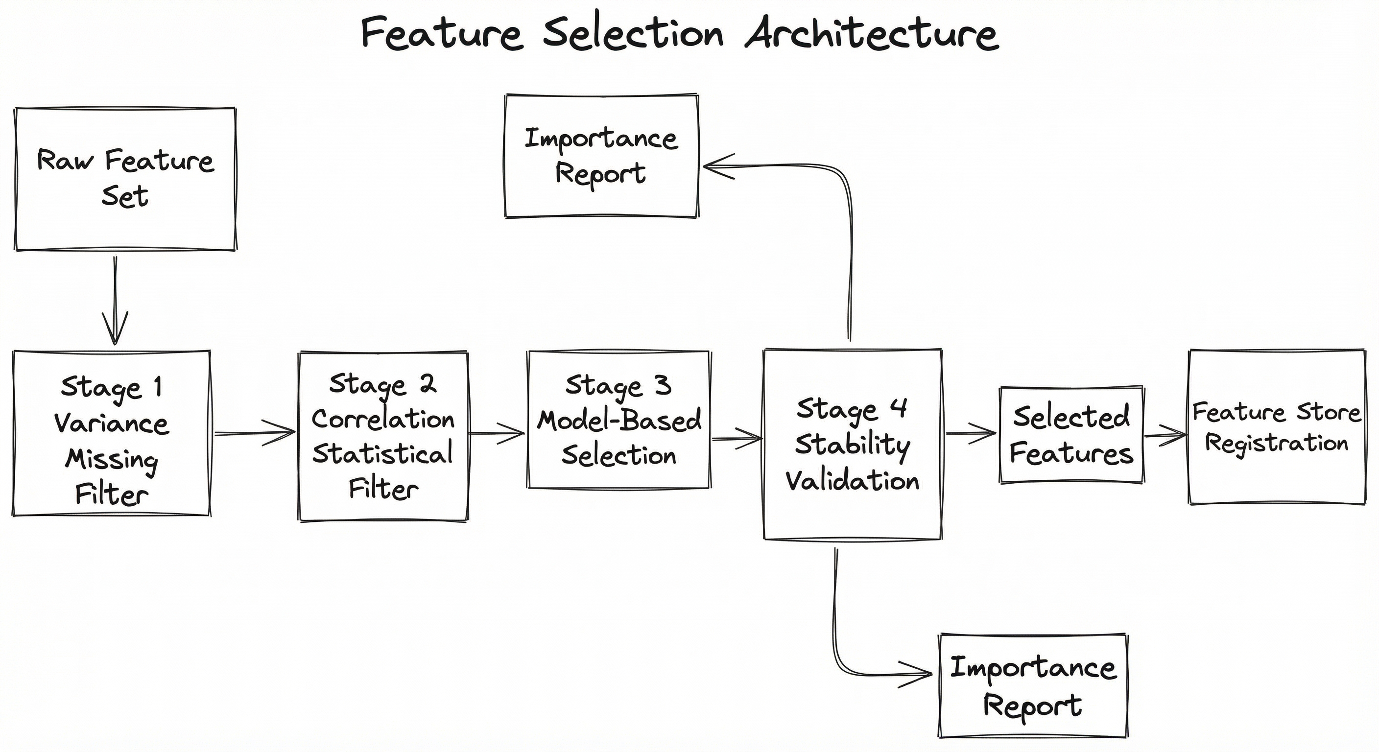
The pipeline follows a funnel architecture: each stage progressively narrows the feature set, with cheaper methods applied first to reduce the candidate pool before expensive model-based methods are invoked. This is critical at scale -- running RFE on 5,000 features is impractical, but running it on the 200 features that survived filter stages is perfectly feasible.
The stability validation stage is often overlooked but essential. It checks whether the selected features are consistent across different data splits, time windows, and random seeds. A feature that is selected in 3 out of 10 cross-validation folds is unreliable and should be flagged.
Key Components
Variance & Missing Value Filter
Removes zero-variance features (constant columns) and features with excessive missing values (>80-90% null). This is a pure data quality check -- no statistical modeling. In sklearn, this is VarianceThreshold. Fast enough to run on billions of rows.
Statistical Filter Engine
Applies univariate statistical tests: Pearson correlation for continuous-continuous pairs, chi-squared for categorical-target pairs, mutual information for general nonlinear dependencies. Removes features below a relevance threshold and highly correlated feature pairs (correlation > 0.95). Implemented via sklearn.feature_selection.SelectKBest or custom pipelines.
Model-Based Selector
Uses embedded or wrapper methods for fine-grained selection. Common choices: RFE with gradient boosting as the estimator, Lasso path with cross-validated lambda, Boruta with Random Forest, or SHAP-based importance from a pre-trained model. This stage captures feature interactions that univariate filters miss.
Stability Validator
Runs the selection pipeline across -fold cross-validation splits and multiple random seeds. Features that appear in >80% of selections are flagged as stable. Generates a stability score for each feature. This prevents selecting features that are artifacts of a particular train/test split.
Feature Importance Reporter
Produces a human-readable report ranking all features by their selection score, noting which stage each dropped feature was eliminated at. This report is essential for audit trails, model documentation, and communication with domain experts who may challenge or validate selections.
Feature Store Integration
Registers the selected feature subset in the feature store (e.g., Feast, Tecton, Vertex AI Feature Store) with metadata about selection method, importance score, and selection date. Enables downstream model training pipelines to consume only the selected features.
Data Flow
Stage 1 (Variance Filter): Raw features ( columns) enter. Features with zero or near-zero variance, and those exceeding the missing value threshold, are dropped. Typical reduction: 10-20% of features removed.
Stage 2 (Statistical Filter): Surviving features are scored using univariate statistical tests against the target variable. Features below the relevance threshold are removed. Highly correlated feature pairs are deduplicated (keeping the one with higher target relevance). Typical reduction: 40-60% of remaining features removed.
Stage 3 (Model-Based Selection): The reduced feature set is fed into one or more model-based selectors (RFE, Lasso, Boruta). These methods capture multivariate interactions and produce a final ranking. Typical reduction: 30-50% of remaining features removed.
Stage 4 (Stability Validation): The selection pipeline is repeated across cross-validation folds. Features appearing in <80% of runs are flagged as unstable. Final output: a stable, validated feature subset with importance scores.
Output: Selected features are registered in the feature store, and the importance report is saved for audit and communication.
A left-to-right funnel showing raw features flowing through four stages: Variance & Missing Value Filter, Correlation & Statistical Filter, Model-Based Selection, and Stability & Validation. The output feeds into Feature Store Registration. A side branch from Model-Based Selection produces a Feature Importance Report.
How to Implement
Practical Implementation Strategies
In practice, feature selection implementation falls into three tiers based on scale and maturity:
Tier 1: Notebook-level exploration (for datasets < 100K rows, < 500 features). Use sklearn's built-in selectors (SelectKBest, RFE, SelectFromModel) interactively. This is where most Kaggle workflows live. Good for prototyping, inadequate for production.
Tier 2: Pipeline-integrated selection (for datasets < 10M rows, < 5,000 features). Build a reproducible pipeline using sklearn Pipeline objects or feature-engine transformers. Selection is run as part of the training pipeline, ensuring the same features are used in training and serving. This is the sweet spot for most startups and mid-size teams.
Tier 3: Automated selection at scale (for datasets > 10M rows, > 5,000 features). Use distributed compute (Spark, Dask) for filter stages, and tools like FeatureWiz or custom mRMR implementations for model-based stages. Selection results are cached in the feature store and versioned. Companies like Uber, Netflix, and Flipkart operate at this tier.
Cost Context: Running a full Boruta selection (100 iterations of Random Forest) on a 1M-row, 1000-feature dataset takes approximately 2-4 hours on an
m5.4xlargeAWS instance (~$0.77/hour, or INR 65/hour). Running the same on ap3.2xlargeGPU instance is unnecessary -- Boruta doesn't benefit from GPU acceleration. Choose your compute wisely.
The code examples below progress from simple filter methods to advanced model-based approaches, each complete and runnable.
import numpy as np
import pandas as pd
from sklearn.feature_selection import (
    VarianceThreshold,
    SelectKBest,
    chi2,
    mutual_info_classif,
)
from sklearn.preprocessing import MinMaxScaler

# Load your dataset
X = pd.DataFrame(np.random.randn(1000, 50), columns=[f"feat_{i}" for i in range(50)])
y = (X["feat_0"] + X["feat_1"] * 2 + np.random.randn(1000) * 0.1 > 0).astype(int)

# Stage 1: Remove near-zero variance features
var_selector = VarianceThreshold(threshold=0.01)
X_var = pd.DataFrame(
    var_selector.fit_transform(X),
    columns=X.columns[var_selector.get_support()],
)
print(f"After variance filter: {X_var.shape[1]} features (from {X.shape[1]})")

# Stage 2a: Chi-squared (requires non-negative features)
X_scaled = MinMaxScaler().fit_transform(X_var)  # Scale to [0, 1]
chi2_selector = SelectKBest(chi2, k=20)
chi2_selector.fit(X_scaled, y)
chi2_scores = pd.Series(chi2_selector.scores_, index=X_var.columns)
print("\nTop 10 features by chi-squared score:")
print(chi2_scores.nlargest(10))

# Stage 2b: Mutual information (handles nonlinear relationships)
mi_selector = SelectKBest(mutual_info_classif, k=20)
mi_selector.fit(X_var, y)
mi_scores = pd.Series(mi_selector.scores_, index=X_var.columns)
print("\nTop 10 features by mutual information:")
print(mi_scores.nlargest(10))

# Get selected features from MI
selected_features = X_var.columns[mi_selector.get_support()].tolist()
print(f"\nSelected {len(selected_features)} features via mutual information")
This example demonstrates the three most common filter methods in a progressive pipeline. VarianceThreshold removes constant or near-constant features in time. Chi-squared measures the dependence between categorical features and the target (requires non-negative inputs, hence the MinMaxScaler). Mutual information captures any statistical dependency, including nonlinear relationships, making it more powerful than chi-squared but slightly slower due to k-NN density estimation. In practice, you would use all three as successive filters.
from sklearn.feature_selection import RFECV
from sklearn.ensemble import GradientBoostingClassifier
from sklearn.model_selection import StratifiedKFold
import matplotlib.pyplot as plt
import pandas as pd
import numpy as np

# Prepare data (assume X, y from previous example)
X = pd.DataFrame(np.random.randn(1000, 50), columns=[f"feat_{i}" for i in range(50)])
y = (X["feat_0"] + X["feat_1"] * 2 + X["feat_2"] * 0.5 + np.random.randn(1000) * 0.3 > 0).astype(int)

# RFE with cross-validation to find optimal number of features
estimator = GradientBoostingClassifier(
    n_estimators=100,
    max_depth=3,
    learning_rate=0.1,
    random_state=42,
)

rfecv = RFECV(
    estimator=estimator,
    step=1,              # Remove 1 feature per iteration
    cv=StratifiedKFold(5, shuffle=True, random_state=42),
    scoring="roc_auc",
    min_features_to_select=5,
    n_jobs=-1,
)

rfecv.fit(X, y)

# Results
print(f"Optimal number of features: {rfecv.n_features_}")
print(f"Selected features: {X.columns[rfecv.support_].tolist()}")
print(f"Feature ranking: {dict(zip(X.columns, rfecv.ranking_))}")

# Plot number of features vs. CV score
plt.figure(figsize=(10, 6))
plt.plot(range(5, len(rfecv.cv_results_['mean_test_score']) + 5),
         rfecv.cv_results_['mean_test_score'])
plt.xlabel('Number of Features')
plt.ylabel('CV ROC-AUC Score')
plt.title('RFECV: Optimal Feature Count')
plt.tight_layout()
plt.savefig('rfecv_plot.png', dpi=150)
print("Plot saved to rfecv_plot.png")
RFECV (Recursive Feature Elimination with Cross-Validation) is the gold standard wrapper method. It trains the model, ranks features by importance, removes the least important feature, and repeats -- using cross-validation to determine when to stop. The step=1 parameter means one feature is removed per iteration (slower but more precise; use step=0.1 to remove 10% per iteration for large feature sets). We use GradientBoostingClassifier as the estimator because tree-based models provide reliable feature importance. The output tells you both which features to keep and the optimal number of features.
import numpy as np
import pandas as pd
from sklearn.linear_model import LassoCV, Lasso
from sklearn.preprocessing import StandardScaler
from sklearn.pipeline import Pipeline

# Prepare data
X = pd.DataFrame(np.random.randn(1000, 50), columns=[f"feat_{i}" for i in range(50)])
y = X["feat_0"] * 3 + X["feat_1"] * 2 + X["feat_2"] * 1.5 + np.random.randn(1000) * 0.5

# Lasso with cross-validated lambda selection
pipeline = Pipeline([
    ("scaler", StandardScaler()),   # Essential: Lasso is scale-sensitive
    ("lasso", LassoCV(
        cv=5,
        alphas=np.logspace(-4, 1, 50),
        max_iter=10000,
        random_state=42,
    )),
])

pipeline.fit(X, y)

lasso_model = pipeline.named_steps["lasso"]
coefficients = pd.Series(lasso_model.coef_, index=X.columns)

# Features with non-zero coefficients are selected
selected = coefficients[coefficients.abs() > 1e-6]
dropped = coefficients[coefficients.abs() <= 1e-6]

print(f"Optimal alpha (lambda): {lasso_model.alpha_:.6f}")
print(f"\nSelected features ({len(selected)}/{len(coefficients)}):")
print(selected.sort_values(ascending=False))
print(f"\nDropped features: {dropped.index.tolist()[:10]}...")
print(f"\nLasso effectively selected {len(selected)} out of {len(coefficients)} features")
Lasso (L1 regularization) is the most widely used embedded method for feature selection. The key insight is that the L1 penalty drives coefficients of irrelevant features to exactly zero (unlike Ridge/L2 which merely shrinks them). LassoCV automatically selects the optimal regularization strength via cross-validation. Critical: always standardize features before Lasso -- otherwise, features with larger scales will be penalized less, leading to incorrect selection. The alphas parameter defines the search grid for the regularization strength.
# pip install boruta
import numpy as np
import pandas as pd
from boruta import BorutaPy
from sklearn.ensemble import RandomForestClassifier

# Prepare data
np.random.seed(42)
n_samples = 2000
X = pd.DataFrame({
    **{f"signal_{i}": np.random.randn(n_samples) for i in range(5)},
    **{f"noise_{i}": np.random.randn(n_samples) for i in range(45)},
})
y = (
    X["signal_0"] * 2 + X["signal_1"] * 1.5 + X["signal_2"] +
    X["signal_3"] * 0.5 + X["signal_4"] * 0.3 +
    np.random.randn(n_samples) * 0.5
> 0).astype(int)

# Initialize Boruta with Random Forest
rf = RandomForestClassifier(
    n_estimators=200,
    n_jobs=-1,
    max_depth=7,
    random_state=42,
)

boruta = BorutaPy(
    estimator=rf,
    n_estimators="auto",
    max_iter=100,         # Maximum iterations
    alpha=0.05,           # Significance level
    random_state=42,
    verbose=2,
)

boruta.fit(X.values, y.values)

# Results
confirmed = X.columns[boruta.support_].tolist()
tentative = X.columns[boruta.support_weak_].tolist()
rejected = X.columns[~boruta.support_ & ~boruta.support_weak_].tolist()

print(f"\nConfirmed features ({len(confirmed)}): {confirmed}")
print(f"Tentative features ({len(tentative)}): {tentative}")
print(f"Rejected features ({len(rejected)}): {rejected[:10]}...")
print(f"\nFeature rankings: {dict(zip(X.columns, boruta.ranking_))}")
Boruta is a wrapper method based on Random Forest that finds all relevant features, not just the top-. It works by creating "shadow features" -- random permutations of each original feature -- and comparing the importance of real features against the maximum importance of shadow features using a statistical test. If a real feature consistently outperforms the best shadow feature, it is confirmed as relevant. This approach is more principled than arbitrary top- selection because it uses a statistical significance test (Bonferroni-corrected). The downside is computational cost: each iteration trains a Random Forest on features.
import numpy as np
import pandas as pd
from sklearn.feature_selection import (
    VarianceThreshold, SelectKBest, mutual_info_classif
)
from sklearn.ensemble import RandomForestClassifier
from sklearn.model_selection import StratifiedKFold
from collections import Counter

def multi_stage_feature_selection(
    X: pd.DataFrame,
    y: pd.Series,
    variance_threshold: float = 0.01,
    mi_top_k: int = 100,
    correlation_threshold: float = 0.95,
    n_folds: int = 5,
    stability_threshold: float = 0.8,
) -> dict:
    """Production-grade multi-stage feature selection pipeline.

    Returns dict with 'selected_features', 'importance_scores',
    'stability_scores', and 'elimination_report'.
    """
    report = {"initial_features": X.shape[1], "stages": []}

    # Stage 1: Variance filter
    var_sel = VarianceThreshold(threshold=variance_threshold)
    var_sel.fit(X)
    surviving = X.columns[var_sel.get_support()].tolist()
    dropped = set(X.columns) - set(surviving)
    report["stages"].append({"name": "variance_filter", "dropped": len(dropped)})
    X_filtered = X[surviving]

    # Stage 2: Remove highly correlated features
    corr_matrix = X_filtered.corr().abs()
    upper_tri = corr_matrix.where(
        np.triu(np.ones(corr_matrix.shape), k=1).astype(bool)
    )
    corr_to_drop = [
        col for col in upper_tri.columns
        if any(upper_tri[col] > correlation_threshold)
    ]
    X_filtered = X_filtered.drop(columns=corr_to_drop)
    report["stages"].append({"name": "correlation_filter", "dropped": len(corr_to_drop)})

    # Stage 3: Mutual information filter
    k = min(mi_top_k, X_filtered.shape[1])
    mi_sel = SelectKBest(mutual_info_classif, k=k)
    mi_sel.fit(X_filtered, y)
    mi_surviving = X_filtered.columns[mi_sel.get_support()].tolist()
    report["stages"].append({
        "name": "mutual_info_filter",
        "dropped": X_filtered.shape[1] - len(mi_surviving),
    })
    X_filtered = X_filtered[mi_surviving]

    # Stage 4: Stability check via cross-validation
    feature_counts = Counter()
    skf = StratifiedKFold(n_splits=n_folds, shuffle=True, random_state=42)

    for train_idx, _ in skf.split(X_filtered, y):
        X_fold = X_filtered.iloc[train_idx]
        y_fold = y.iloc[train_idx]

        rf = RandomForestClassifier(n_estimators=100, random_state=42, n_jobs=-1)
        rf.fit(X_fold, y_fold)

        importances = pd.Series(rf.feature_importances_, index=X_filtered.columns)
        top_features = importances.nlargest(k // 2).index.tolist()
        feature_counts.update(top_features)

    stability_scores = {
        feat: count / n_folds for feat, count in feature_counts.items()
    }
    stable_features = [
        feat for feat, score in stability_scores.items()
        if score >= stability_threshold
    ]

    report["stages"].append({
        "name": "stability_validation",
        "stable_features": len(stable_features),
    })
    report["final_features"] = len(stable_features)

    return {
        "selected_features": stable_features,
        "stability_scores": stability_scores,
        "elimination_report": report,
    }


# Usage
X = pd.DataFrame(np.random.randn(5000, 200), columns=[f"f_{i}" for i in range(200)])
y = pd.Series((X["f_0"] + X["f_1"] * 2 + np.random.randn(5000) * 0.3 > 0).astype(int))

result = multi_stage_feature_selection(X, y, mi_top_k=50)
print(f"Selected {len(result['selected_features'])} stable features from 200")
print(f"Elimination report: {result['elimination_report']}")
This production-ready pipeline implements the funnel architecture described earlier. It chains four stages: variance filtering, correlation-based deduplication, mutual information scoring, and cross-validated stability checking using Random Forest importance. The stability check ensures features are consistently selected across data splits, preventing overfitting to a particular train/test partition. The elimination report provides a full audit trail showing how many features were dropped at each stage -- essential for debugging and compliance in regulated industries like fintech.
# Feature selection pipeline config (YAML)
feature_selection:
  stages:
    - name: variance_filter
      threshold: 0.01
      enabled: true

    - name: missing_value_filter
      max_missing_rate: 0.80
      enabled: true

    - name: correlation_filter
      method: pearson
      threshold: 0.95
      keep: higher_mi_with_target
      enabled: true

    - name: statistical_filter
      method: mutual_info  # Options: chi2, f_classif, mutual_info
      top_k: 100
      enabled: true

    - name: model_based_selection
      method: rfecv  # Options: rfecv, boruta, lasso, shap
      estimator: gradient_boosting
      cv_folds: 5
      scoring: roc_auc
      enabled: true

    - name: stability_check
      n_folds: 10
      n_seeds: 3
      min_stability: 0.80
      enabled: true

  output:
    feature_list_path: artifacts/selected_features.json
    importance_report_path: artifacts/feature_importance.html
    register_to_feature_store: true
    feature_store_project: fraud-detection-v2
Common Implementation Mistakes
- ●
Data leakage during feature selection: Performing feature selection on the entire dataset (including test data) before splitting. This causes the selection process to 'peek' at test data, leading to overly optimistic evaluation metrics. Always run feature selection inside cross-validation folds or on the training set only.
- ●
Ignoring feature interactions: Relying solely on univariate filter methods (correlation, chi-squared) that evaluate each feature independently. Features that are individually weak predictors can be powerful in combination. Always follow filter methods with a model-based method that captures interactions.
- ●
Not standardizing before Lasso: L1 regularization penalizes coefficients proportionally, so features on larger scales receive less regularization. Always apply
StandardScalerbefore Lasso-based selection -- this is a hard requirement, not a best practice. - ●
Treating feature selection as a one-time task: In production, data distributions drift over time. A feature that was critical six months ago may become irrelevant (or vice versa). Schedule periodic re-selection -- monthly or quarterly -- and track feature importance trends.
- ●
Using too many features in the initial RFE: Running Recursive Feature Elimination on thousands of features is computationally prohibitive ( model training iterations). Use filter methods first to reduce to 100-200 candidates, then apply RFE.
- ●
Confusing feature importance with causation: A feature with high Random Forest importance or high SHAP value is a strong predictor, not necessarily a causal driver. Feature selection identifies association, not causation. Making business decisions based on feature importance without causal analysis can be misleading.
When Should You Use This?
Use When
Your dataset has more than 50 features and you suspect many are irrelevant or redundant -- this is the most common trigger for feature selection.
Model training time is a bottleneck: reducing features from 1,000 to 100 can cut training time by 5-10x for tree-based models and even more for linear models.
You need interpretable models for regulatory compliance (e.g., credit scoring under RBI guidelines in India, or GDPR right-to-explanation in Europe) and must justify each input feature.
Inference latency is critical: in real-time serving (e.g., Razorpay fraud detection at checkout, requiring <200ms decisions), fewer features mean fewer feature store lookups and faster predictions.
Your model is overfitting: high training accuracy but poor validation/test performance is a classic symptom of too many noisy features.
Feature computation is expensive: some features require joins across multiple tables, API calls, or complex aggregations. Eliminating unnecessary ones directly reduces your data pipeline cost.
You are deploying to resource-constrained environments (mobile, edge devices) where model size and feature computation budgets are limited.
Avoid When
Your feature set is already small and curated (< 20 features hand-selected by domain experts). Feature selection adds complexity without meaningful benefit.
You are using deep learning models that learn their own feature representations (CNNs, Transformers). These models perform implicit feature selection through their architecture. Explicit feature selection on raw pixels or tokens is counterproductive.
Your problem requires all available information (e.g., genomics where every gene could matter, or rare event detection where subtle signals in many features must be preserved).
You are performing exploratory data analysis and don't yet have a clear target variable. Feature selection is inherently target-dependent.
The features are already the output of a dimensionality reduction method (PCA, autoencoders). These are already compressed representations; further selection can destroy the structure.
You have a very large dataset relative to features (n >> p) and your model has built-in regularization. In this regime, overfitting due to excess features is less of a concern.
Key Tradeoffs
Accuracy vs. Interpretability
Aggressive feature selection (keeping only 10-20 features) produces highly interpretable models that are easy to explain to stakeholders and regulators. But it may miss subtle feature interactions that a richer feature set would capture. The sweet spot depends on your use case: a credit scoring model at a bank needs maximal interpretability, while a recommendation engine can tolerate a black box with more features.
Computation Time vs. Selection Quality
| Method | Compute Cost | Selection Quality | Interaction Capture |
|---|---|---|---|
| Variance Threshold | Very Low | Low (data quality only) | None |
| Correlation Filter | Low | Medium | Pairwise only |
| Chi-Squared / MI | Low-Medium | Medium-High | None (univariate) |
| mRMR | Medium | High | Pairwise redundancy |
| Lasso | Medium | High (for linear models) | Linear interactions |
| RFE | High | Very High | Full (model-dependent) |
| Boruta | Very High | Very High | Full (Random Forest) |
| SHAP-based | Very High | Very High | Full (model-agnostic) |
Stability vs. Aggressiveness
More aggressive selection (fewer features) increases the risk of instability -- small changes in training data can lead to different feature subsets. This is a real production concern. If your feature set changes every time you retrain, your monitoring dashboards, alerting rules, and downstream dependencies all break. The stability validation stage in the pipeline architecture addresses this, but at the cost of being more conservative in selection.
Practical Guideline: Start with filter methods to get a quick baseline. If model performance is acceptable, stop there. If not, add model-based selection. Only use Boruta or SHAP-based selection when you need statistical rigor about which features are truly relevant (e.g., for a research paper or regulatory submission).
Alternatives & Comparisons
Feature extraction creates new features from combinations of existing ones (e.g., PCA produces orthogonal principal components). Feature selection keeps a subset of original features unchanged. Choose feature extraction when interpretability of individual features doesn't matter and you need maximum dimensionality reduction. Choose feature selection when you need to explain which original features drive predictions, monitor individual features for drift, and maintain operational simplicity.
A feature store is the infrastructure that stores, serves, and versions features. Feature selection is the process that decides which features to include. They are complementary: feature selection determines the feature set; the feature store operationalizes it. Every production system needs both -- selection to curate, and a store to serve.
Feature scaling transforms feature values to comparable ranges (StandardScaler, MinMaxScaler) but does not remove features. Feature selection removes features entirely. They often work together: scaling is a prerequisite for Lasso-based feature selection (L1 regularization is scale-sensitive). Apply scaling first, then selection.
Regularized models (L1/L2, dropout, early stopping) implicitly handle irrelevant features by shrinking their contribution. If you are using a well-regularized model like XGBoost or a neural network with dropout, explicit feature selection may provide diminishing returns. However, feature selection still reduces serving latency and operational complexity, which regularization alone does not address.
Pros, Cons & Tradeoffs
Advantages
Reduces overfitting by removing noisy and irrelevant features, leading to better generalization on unseen data. In practice, dropping 50-70% of features often improves validation metrics.
Decreases training time proportionally to the number of features removed. For tree-based models, halving the feature count roughly halves training time. For linear models, the speedup can be even greater.
Improves model interpretability -- a model with 15 selected features is far easier to explain to business stakeholders than one with 500. This is critical for regulated industries (banking, insurance, healthcare).
Reduces serving latency and infrastructure cost by requiring fewer feature lookups and less memory at inference time. At Flipkart's scale (millions of predictions/day), removing 100 unnecessary features could save INR 50,000-2,00,000 (~$600-2,400) per month in compute.
Simplifies monitoring and debugging -- fewer features mean fewer data pipelines to maintain, fewer drift alerts to manage, and faster root cause analysis when model performance degrades.
Enables deployment on resource-constrained devices -- mobile apps, IoT sensors, and edge devices have strict memory and compute budgets. Feature selection is essential for on-device ML.
Identifies the most important predictive signals in your data, providing valuable domain insights even beyond model building.
Disadvantages
Risk of removing informative features -- no selection method is perfect. Univariate methods may drop features that are only useful in combination. This is especially dangerous with filter methods that ignore feature interactions.
Computational cost of wrapper methods -- RFE and Boruta require multiple rounds of full model training, which can be prohibitive for large datasets. Boruta on a 1M-row, 1000-feature dataset can take hours.
Selection instability -- different random seeds, data samples, or cross-validation folds may yield different feature subsets. This makes the pipeline less reproducible and harder to version.
Target-dependent selection -- features selected for one target (e.g., click-through rate) may not be optimal for another (e.g., conversion rate). Multi-task systems need separate selection or a unified approach.
Potential for data leakage if selection is not properly integrated into the cross-validation pipeline. This is one of the most common and most costly mistakes in ML pipelines.
Requires careful tuning -- thresholds for variance, correlation, significance levels, and number of features to select are all hyperparameters that need tuning. Bad defaults can lead to either too few or too many features.
Failure Modes & Debugging
Data leakage through improper selection scope
Cause
Feature selection is performed on the entire dataset (including test/validation data) before the train-test split. The selection process learns information from the test set, leading to overly optimistic performance estimates.
Symptoms
Model performs significantly better in offline evaluation than in production. Validation metrics are suspiciously close to training metrics. Performance drops sharply when deployed on truly unseen data.
Mitigation
Always perform feature selection inside the cross-validation loop or strictly on the training fold. Use sklearn.pipeline.Pipeline to ensure selection and training are coupled. Implement a strict "no peeking" policy in your ML pipeline code.
Univariate filter misses interaction effects
Cause
Using only filter methods (chi-squared, correlation) that evaluate each feature independently. Two features that are individually weak predictors may be powerful together (e.g., age and income jointly predict loan default better than either alone).
Symptoms
Model performance plateaus despite having many candidate features. Adding features manually (based on domain knowledge) that were dropped by the filter improves performance significantly.
Mitigation
Layer filter methods with model-based methods (RFE, Boruta, or tree importance) that naturally capture interactions. Use mRMR which at least accounts for pairwise redundancy. Always validate filter-selected subsets with a downstream model evaluation.
Lasso selects arbitrarily among correlated features
Cause
When features are highly correlated (multicollinear), Lasso tends to select one feature from each correlated group and zero out the rest -- but the choice of which feature is arbitrary and unstable across runs.
Symptoms
Different Lasso runs (different random seeds or slightly different data) select different features from correlated groups. The selected feature set is not reproducible.
Mitigation
Use Elastic Net (combination of L1 and L2) which handles multicollinearity better by encouraging group selection. Alternatively, remove highly correlated features (correlation > 0.95) before applying Lasso. Or use group Lasso when you know the correlation structure.
Feature drift makes selection stale
Cause
Feature selection was performed on historical data, but the data distribution has shifted over time. Features that were informative during selection are no longer predictive in the current distribution.
Symptoms
Model performance gradually degrades over weeks/months. Feature importance rankings in production diverge significantly from those at selection time. Re-running selection on recent data produces a substantially different feature set.
Mitigation
Implement periodic re-selection (monthly or quarterly). Monitor feature importance in production and set alerts when importance rankings shift by more than 20%. Use a sliding window of recent data for selection rather than a static historical dataset.
Boruta/RFE timeout on high-dimensional data
Cause
Running wrapper methods directly on very high-dimensional data (>5,000 features) without pre-filtering. Boruta creates 2p shadow features and trains a Random Forest on all of them; RFE trains models.
Symptoms
Feature selection job runs for hours or days without completing. Memory usage spikes as shadow features double the feature matrix. The pipeline times out or gets killed by the scheduler.
Mitigation
Always apply cheap filter methods (variance threshold, correlation filter) to reduce the feature set to <500 features before running wrapper methods. For Boruta, set max_iter=50 and use n_estimators=100 (not the default 'auto' which can be very high). Consider using BorutaShap which is faster than classic Boruta.
Selection bias toward high-cardinality features
Cause
Tree-based feature importance (used in RFE, Boruta, and SelectFromModel with Random Forest) is biased toward features with many unique values or high cardinality. Continuous features and high-cardinality categoricals receive inflated importance scores.
Symptoms
Categorical features with few levels (e.g., binary flags) are consistently ranked low despite domain knowledge suggesting they are important. Features like user IDs or timestamps receive high importance due to cardinality, not predictive power.
Mitigation
Use permutation importance instead of impurity-based importance, as it is unbiased with respect to cardinality. In sklearn, use sklearn.inspection.permutation_importance. Alternatively, use SHAP values which are also cardinality-agnostic.
Placement in an ML System
Where Feature Selection Sits in the ML Pipeline
Feature selection occupies a critical position between feature engineering/extraction (upstream) and model training (downstream). It is the gatekeeper that determines which features actually make it into the model.
In a typical production pipeline at a company like Flipkart or Swiggy:
- Feature extraction generates raw features from data sources (user behavior logs, transaction records, item catalogs).
- Feature store catalogs and serves these features.
- Feature selection evaluates which features to include in a specific model.
- Model training consumes only the selected features.
Importantly, feature selection feeds back into the feature store: once a feature is confirmed as irrelevant across multiple models, the team can deprecate its computation pipeline, saving ongoing compute costs.
Operational Insight: At scale, the feedback loop from feature selection to feature store deprecation is where the real cost savings happen. A feature that no model uses but is still being computed daily is pure waste. Companies like Uber have saved significant infrastructure costs by systematically pruning unused features from their feature store (Palette) based on selection results.
Pipeline Stage
Feature Engineering / Preprocessing
Upstream
- feature-extraction
- feature-store
- scaling
Downstream
- model-training
- feature-store
Scaling Bottlenecks
The primary bottleneck is computation time for wrapper methods at scale. Boruta on a dataset with 1M rows and 1,000 features requires training ~100 Random Forests, each on 2,000 features (originals + shadows) -- this can take 4-8 hours on a single machine. The solution is a two-phase approach: run cheap filter methods on the full feature set (minutes), then run expensive wrapper methods on the filtered subset (minutes to an hour).
For filter methods, the bottleneck shifts to memory when computing pairwise correlation matrices. A 10,000-feature dataset requires a 10,000 x 10,000 correlation matrix (~800 MB in float64). At 50,000 features, that's ~20 GB. Use chunked computation or sampling strategies for very high-dimensional data.
At extreme scale (>100M rows), even mutual information estimation becomes expensive. Uber's approach of using distributed mRMR computation on Spark addresses this -- but adds infrastructure complexity.
Production Case Studies
Uber developed X-Ray, an information-theoretic feature discovery tool built on the mRMR (Minimum Redundancy Maximum Relevance) algorithm. X-Ray automatically ranks features from Uber's Palette feature store (containing hundreds of tables with up to 1,000 features each) to identify compact, diverse feature subsets for ML models across marketing, pricing, and ETA prediction.
By applying mRMR-based selection, Uber reduced a marketing model's feature set from 75 to 37 features while achieving significantly higher performance (measured by AUC). The 37-feature model included 15 original features and 22 newly discovered ones from the feature store, demonstrating that selection is not just about removal but also about discovering overlooked signal.
Razorpay's fraud detection system (Thirdwatch) processes millions of transactions daily with real-time feature generation using Apache Flink. Feature selection is critical here -- with 800+ candidate features extracted from transaction data, device fingerprints, and behavioral signals, they use a combination of domain expert curation and model-based selection (XGBoost feature importance) to select the ~100-150 features that actually reach the fraud scoring model.
The feature selection pipeline enables Razorpay to serve fraud decisions in under 200ms at checkout -- a latency budget that would be impossible with the full 800-feature set. Selected features are served via Flink feature generation into XGBoost and rule engine models in real-time.
Netflix consolidated multiple recommendation models into a single unified multi-task model. A critical step in this consolidation was feature selection and harmonization across previously independent models. They used a combination of feature importance analysis and ablation studies to identify the core feature set that served all recommendation tasks (row selection, artwork personalization, video ranking) without degradation.
The consolidated model with a carefully selected shared feature set matched or exceeded the performance of the individual specialized models while dramatically simplifying the serving infrastructure. Feature selection enabled this consolidation by identifying the 'universal' features that carry signal across multiple tasks.
Flipkart's product ranking and recommendation systems operate on thousands of features derived from user behavior, product attributes, and contextual signals. Their ML platform team implemented an automated feature selection pipeline that runs filter methods (correlation-based deduplication) followed by tree-based importance ranking to reduce the feature set for each model variant. This is integrated into their model training workflow so that selection is re-run with each retrain cycle.
Automated feature selection reduced the average model's feature count by ~40% while maintaining ranking quality (NDCG), cutting feature store read costs and reducing model serving latency by approximately 25%. The automation eliminated manual feature curation, which had been a bottleneck requiring senior data scientist time.
Tooling & Ecosystem
The most comprehensive feature selection toolkit in Python. Includes VarianceThreshold, SelectKBest (with chi2, f_classif, mutual_info_classif scoring), RFE, RFECV, SelectFromModel, and SequentialFeatureSelector. The standard starting point for any feature selection workflow.
Python implementation of the Boruta all-relevant feature selection algorithm. Wraps around any sklearn-compatible classifier (typically Random Forest). Identifies all features that are statistically more relevant than random noise, rather than selecting a fixed top-.
sklearn-compatible library for feature engineering and selection. Provides specialized selectors including DropCorrelatedFeatures, SmartCorrelatedSelection, SelectByShuffling, RecursiveFeatureElimination, and SelectByTargetMeanPerformance. Designed for production pipelines with clean APIs.
Automated feature selection library powered by the SULOV (Searching for Uncorrelated List of Variables) algorithm combined with recursive XGBoost. Selects features with high mutual information to the target and low inter-feature correlation. One-line API: featurewiz(dataframe, target). Built by Ram Seshadri.
Fast Python implementation of the mRMR algorithm for feature selection. Supports both classification and regression. Efficiently handles large datasets using pandas and category_encoders. Used in production at companies like Uber for information-theoretic feature ranking.
While primarily an explainability library, SHAP values provide model-agnostic feature importance that is theoretically grounded in game theory (Shapley values). Using shap.summary_plot and mean absolute SHAP values for feature ranking is increasingly popular for feature selection in production, as it accounts for feature interactions and is unbiased toward high-cardinality features.
XGBoost provides three types of feature importance: weight (number of times a feature appears in trees), gain (average improvement in accuracy when the feature is used), and cover (average number of samples affected). Gain-based importance is most commonly used for feature selection.
Research & References
Robert Tibshirani (1996)Journal of the Royal Statistical Society: Series B, Vol. 58
The seminal paper introducing Lasso (L1 regularization) for simultaneous regression shrinkage and variable selection. Showed that the L1 penalty produces sparse solutions with exactly zero coefficients, enabling automatic feature selection during model training.
Miron B. Kursa, Witold R. Rudnicki (2010)Journal of Statistical Software, Vol. 36, Issue 11
Introduced the Boruta algorithm for all-relevant feature selection using shadow variables and Random Forest. Boruta compares feature importance against randomized copies to determine statistical significance, finding all features that are genuinely informative rather than just the top-.
Zhenyu Zhao, Radhika Anand, Mallory Wang (2019)KDD 2019 Workshop
Describes Uber's production implementation of mRMR-based feature selection for marketing ML models. Demonstrates how information-theoretic feature ranking scales to large feature stores with thousands of candidate features, achieving better model performance with fewer features.
Maximilian Stubbemann, Tom Hanika, Gerd Stumme (2023)arXiv preprint
Proposes a novel feature selection method that identifies features allowing discrimination of data subsets at different scales, directly addressing the curse of dimensionality. Adapts intrinsic dimensionality estimation to rank features by their ability to preserve meaningful distances in high-dimensional spaces.
Isabelle Guyon, Andre Elisseeff (2003)Journal of Machine Learning Research, Vol. 3
The foundational survey paper on feature selection in machine learning. Provides a comprehensive taxonomy of filter, wrapper, and embedded methods. Introduced practical guidelines and the distinction between feature ranking (scoring individual features) and feature subset selection (finding optimal combinations). Still widely cited as the definitive reference.
Andrew Y. Ng (2004)ICML 2004
Provides theoretical analysis of why L1 regularization leads to sparse solutions (feature selection) while L2 does not. Shows that L1 is more appropriate when the number of irrelevant features is large relative to the number of training examples, and that L2 is rotationally invariant while L1 is not.
Interview & Evaluation Perspective
Common Interview Questions
- ●
What are the three main categories of feature selection methods? When would you use each?
- ●
How does Lasso (L1 regularization) perform feature selection? Why does L1 produce sparse solutions while L2 does not?
- ●
You have a dataset with 1,000 features. Walk me through your feature selection strategy.
- ●
What is the curse of dimensionality and how does feature selection address it?
- ●
How do you handle feature selection when features are highly correlated (multicollinear)?
- ●
What is the difference between feature selection and feature extraction (PCA)? When would you prefer one over the other?
- ●
How would you implement feature selection in a production ML pipeline to prevent data leakage?
- ●
Your model uses 200 features. The business wants to reduce this to 20 for interpretability. How do you approach this?
Key Points to Mention
- ●
Feature selection methods form a spectrum: filter (fast, univariate) -> wrapper (accurate, expensive) -> embedded (balanced, model-dependent). Production systems typically use a multi-stage funnel combining all three.
- ●
Data leakage is the #1 pitfall: feature selection must happen inside cross-validation, not before the train-test split. This is a common mistake even among experienced practitioners.
- ●
Lasso produces sparse solutions because the L1 penalty creates corner solutions at the axes of the coefficient space, where some coefficients are exactly zero. L2 penalty creates spherical contours that rarely intersect axes. Draw the diamond (L1) vs. circle (L2) diagram.
- ●
Mutual information is strictly more powerful than correlation for feature selection because it captures nonlinear dependencies. But it requires more samples for accurate estimation.
- ●
Boruta is the gold standard for all-relevant feature selection -- it uses statistical testing against shadow features rather than arbitrary top- cutoffs.
- ●
In production, feature selection is not a one-time step -- it must be re-run periodically to account for data drift and changing feature relevance.
Pitfalls to Avoid
- ●
Saying 'just use PCA' when asked about feature selection -- PCA is dimensionality reduction via projection, not feature selection. They solve different problems.
- ●
Ignoring the computational cost of wrapper methods -- claiming you would run Boruta on 10,000 features without mentioning the need for pre-filtering.
- ●
Treating filter methods as sufficient on their own -- they miss feature interactions. Always mention the need for model-based validation.
- ●
Forgetting to mention data leakage prevention -- this is the most important practical consideration and interviewers expect you to bring it up proactively.
- ●
Not discussing stability -- mentioning that selected features should be consistent across data splits shows production experience.
Senior-Level Expectation
A senior/staff-level candidate should articulate the full production lifecycle of feature selection: (1) initial selection using a multi-stage funnel (filter -> wrapper/embedded -> stability check), (2) integration with the training pipeline via sklearn Pipeline or similar abstractions to prevent leakage, (3) monitoring of feature importance in production with drift detection, (4) periodic re-selection with A/B testing to validate that new feature sets improve production metrics, and (5) cost-aware selection that considers not just predictive power but also feature computation cost, serving latency impact, and operational maintenance burden. The candidate should be able to discuss tradeoffs specific to their domain (e.g., in fintech, regulatory requirements for feature interpretability; in ad-tech, the need for ultra-low latency; in healthcare, the importance of clinical interpretability). They should mention tools like mRMR, SHAP-based selection, and Boruta, and articulate when each is appropriate. Bonus points for discussing how feature selection interacts with the feature store -- specifically, the feedback loop where selection results inform feature deprecation decisions.
Summary
Feature selection is the disciplined practice of identifying and retaining only the most informative variables in a dataset -- a process that directly impacts model accuracy, training efficiency, serving latency, and operational simplicity. It is one of the highest-leverage activities in any ML pipeline, yet it is frequently under-invested in production systems.
The three families of methods -- filter (chi-squared, mutual information, correlation), wrapper (RFE, Boruta), and embedded (Lasso, tree importance) -- form a spectrum of increasing accuracy and computational cost. The production best practice is a multi-stage funnel: cheap filter methods for initial screening, followed by model-based methods for fine-grained selection, validated through cross-fold stability checks. This architecture scales from startup prototypes to systems like Uber's X-Ray platform that ranks thousands of features from a massive feature store.
The critical implementation considerations are: (1) prevent data leakage by performing selection inside cross-validation folds, (2) combine methods rather than relying on any single technique, (3) validate stability across data splits and time windows, (4) re-run periodically to account for data drift, and (5) close the feedback loop by deprecating unused features from the feature store. Whether you are building a fraud detection system at Razorpay that must respond in 200ms, a recommendation engine at Flipkart that ranks millions of products, or a credit scoring model that must satisfy RBI regulatory requirements for interpretability -- feature selection is the bridge between raw feature abundance and production-ready, efficient, trustworthy ML models.