Image Preprocessor in Machine Learning
Every computer vision model -- whether it detects tumors in chest X-rays or identifies counterfeit products on Flipkart -- begins its life with a deceptively simple question: how should we prepare the raw pixels before feeding them to the network?
The image preprocessor is the block that answers this question. It sits at the very front of any CV pipeline, transforming raw images from disk, camera, or network into the precise tensor format a model expects: correct spatial dimensions, normalized pixel distributions, consistent color space, and optionally augmented with geometric or photometric perturbations to improve generalization.
This sounds trivial until you realize that a mismatch in normalization statistics can silently drop your model's accuracy by 5-10%, that the wrong resizing interpolation can introduce aliasing artifacts that confuse object detectors, and that a poorly designed preprocessing pipeline can become the single biggest bottleneck in your training loop -- leaving expensive GPUs idle 40-60% of the time while the CPU struggles to decode and transform images.
From Swiggy's food image classification to Tesla's Autopilot camera calibration, image preprocessing is the invisible foundation that determines the quality ceiling of everything downstream. Get it right and your model trains faster, generalizes better, and serves reliably. Get it wrong and no amount of architecture tuning will save you.
Concept Snapshot
- What It Is
- A pipeline component that transforms raw images into model-ready tensors through resizing, normalization, color conversion, and optional augmentation.
- Category
- Computer Vision
- Complexity
- Intermediate
- Inputs / Outputs
- Inputs: raw images (JPEG, PNG, DICOM, RAW) of arbitrary sizes and color spaces. Outputs: batched tensors of fixed spatial dimensions with normalized pixel values, ready for model consumption.
- System Placement
- Sits at the very beginning of a CV pipeline, after data loading and before the model's forward pass (training) or inference engine (serving).
- Also Known As
- image transform pipeline, image preprocessing pipeline, data preprocessing (vision), input normalization, image preparation, pixel preprocessing
- Typical Users
- ML Engineers, Computer Vision Engineers, Data Scientists, MLOps Engineers, Research Scientists
- Prerequisites
- Basic image representation (pixels, channels, color spaces), Tensor operations (reshape, transpose, normalize), Understanding of CNN input requirements, Familiarity with PyTorch or TensorFlow data loading
- Key Terms
- normalizationstandardizationinterpolationaugmentationletterboxingcolor space conversionImageNet statisticstorchvision transformsalbumentationsDALI
Why This Concept Exists
The Gap Between Raw Pixels and Model Expectations
A raw image from a smartphone camera might be 4032x3024 pixels, encoded as a JPEG with 8-bit sRGB color, and weigh 3-5 MB. A ResNet-50 expects a 224x224x3 float32 tensor with pixel values centered around zero. An object detector like YOLOv8 expects 640x640 with values in [0, 1]. A medical imaging model might need 512x512 grayscale with Hounsfield unit normalization.
The image preprocessor bridges this gap. Without it, you would need to manually handle every transformation for every model, every dataset, and every deployment environment -- a combinatorial nightmare.
Three Problems That Made This Critical
Problem 1: Consistency. Neural networks are surprisingly sensitive to input distribution shifts. If your training pipeline normalizes with ImageNet statistics (mean=[0.485, 0.456, 0.406], std=[0.229, 0.224, 0.225]) but your serving pipeline divides by 255.0 and calls it a day, your model will silently produce garbage predictions. No error, no warning -- just wrong answers. This has bitten more production teams than any architecture bug.
Problem 2: Speed. A naive preprocessing pipeline that decodes JPEG, resizes, normalizes, and augments images sequentially on a single CPU core can process maybe 100-200 images per second. A modern GPU can consume 1,000-5,000 images per second during training. That 5-50x gap means your $2-4/hour GPU (~INR 170-340/hour) sits idle most of the time, burning money while waiting for data. This is why libraries like NVIDIA DALI exist -- they move preprocessing to the GPU, eliminating the CPU bottleneck entirely.
Problem 3: Augmentation for generalization. Real-world images come with variable lighting, angles, occlusions, and noise. A model trained only on pristine, well-lit studio photos will fail spectacularly when deployed to a warehouse camera with poor lighting or a phone camera with motion blur. Data augmentation -- random flips, rotations, color jitter, cutout, mixup -- simulates this variability during training, dramatically improving robustness. But augmentation must be applied correctly: you don't flip a document OCR image horizontally, and you don't randomly crop when training an object detector without adjusting bounding boxes.
Historical Evolution
Early deep learning preprocessing was ad hoc -- a few lines of OpenCV or PIL code at the top of a training script. As models grew and datasets scaled to millions of images, the community realized that preprocessing needed its own abstraction:
- 2012-2015: Manual OpenCV/PIL preprocessing. AlexNet's preprocessing was a few lines of center-crop and mean subtraction.
- 2016-2018:
torchvision.transformsandtf.imageprovided composable transform APIs. Still CPU-bound. - 2018-2020: Albumentations brought fast, NumPy-optimized augmentations with bounding box and mask support. AutoAugment and RandAugment automated augmentation policy search.
- 2020-present: NVIDIA DALI moved the entire pipeline to GPU.
torchvision.transforms.v2unified transforms across images, boxes, masks, and video. Preprocessing became a first-class engineering concern, not an afterthought.
Key Takeaway: Image preprocessing exists because raw pixels and model expectations live in different worlds. The preprocessor is the translator between them -- and its quality directly determines your model's quality ceiling.
Core Intuition & Mental Model
The Mental Model: A Factory Assembly Line
Think of image preprocessing as an assembly line in a factory. Raw images arrive at the loading dock in all shapes and sizes -- some wrapped in JPEG compression, some in PNG, some enormous, some tiny, some shot in daylight, others in artificial lighting. The assembly line standardizes them into uniform, model-ready products.
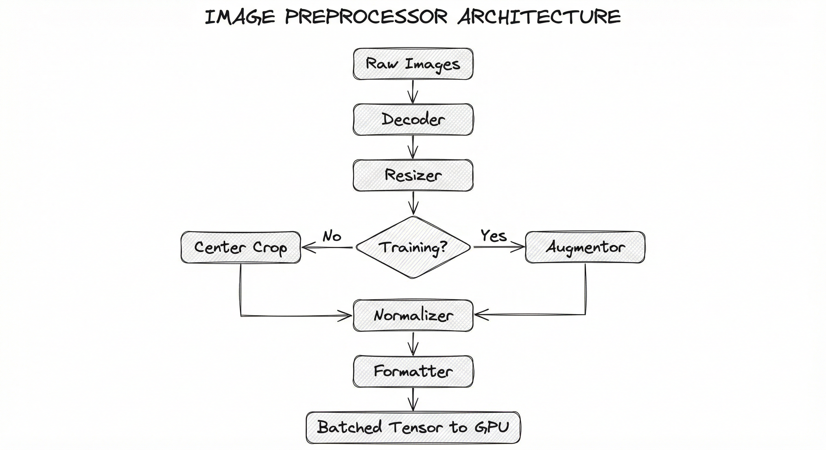
Station 1 (Decode): Unwrap the compressed format into raw pixel arrays. Station 2 (Resize): Stamp every image to the same spatial dimensions. Station 3 (Normalize): Calibrate the pixel values to a known distribution. Station 4 (Augment, training only): Introduce controlled randomness to build robustness. Station 5 (Format): Convert to the tensor format the model consumes (CHW vs HWC, float32 vs float16).
Skip a station and the product is defective. Run the stations in the wrong order and you get unexpected results. Operate the stations too slowly and the entire factory (your GPU) sits idle.
Why Order Matters
Here is a subtlety that trips up even experienced engineers: the order of preprocessing operations matters enormously. Consider normalization and augmentation. If you normalize first (subtract mean, divide by std) and then apply a random brightness shift, you are shifting already-normalized values, which can push pixels outside the expected distribution. The correct order is almost always: decode -> resize -> augment -> normalize -> convert to tensor.
Similarly, resizing before augmentation is usually preferred because spatial augmentations (rotation, affine transforms) are faster on smaller images and produce more predictable results.
The Invisible Contract
Every pretrained model has an implicit preprocessing contract: the exact sequence of operations that were applied to training data. When you use a pretrained model, you must honor this contract exactly. If ResNet-50 was trained with bilinear resize to 256, center crop to 224, and ImageNet normalization, your inference pipeline must do the same -- not bicubic resize to 224, not [0, 1] normalization. Violating this contract is the number one cause of "my model works in training but fails in production" bugs.
Expert Note: When debugging unexpected model behavior, the first thing to check is whether training and inference preprocessing pipelines are identical. Serialize your preprocessing config (as a YAML or JSON file) and version-control it alongside your model checkpoint. This one practice prevents more production incidents than any monitoring system.
Technical Foundations
Mathematical Formulation
Let be a raw input image with height , width , and channels (typically for RGB). The image preprocessor applies a composition of transformations to produce a model-ready tensor :
Core Transformations
Resizing. Given target dimensions , resizing maps to via an interpolation kernel :
where is the neighborhood of pixels contributing to the output. For bilinear interpolation, (2x2 neighborhood). For bicubic, (4x4 neighborhood). For nearest neighbor, .
Normalization. Channel-wise standardization transforms each pixel in channel :
For ImageNet-pretrained models, the canonical values are:
These were computed across the 1.28 million training images in ILSVRC-2012. The normalization ensures that each channel has approximately zero mean and unit variance, which stabilizes gradient flow during training.
Color Space Conversion. RGB to grayscale uses the luminance formula:
RGB to HSV, RGB to LAB, and other conversions follow standard colorimetry transforms. The choice of color space can significantly affect model performance: HSV separates color from intensity (useful for lighting-invariant features), while LAB approximates human perceptual uniformity.
Augmentation. Let be a set of stochastic augmentation operations. At training time, a subset is sampled and applied:
where each is a random transformation parameterized by magnitude and probability . For example, RandAugment selects operations uniformly from , each with a shared magnitude -- reducing the search space from in AutoAugment to just two hyperparameters .
Computational Complexity
For a batch of images resized to :
- Bilinear resize: -- four multiplications per output pixel
- Normalization: -- one subtract and one divide per pixel
- JPEG decode: -- inverse DCT is the bottleneck, typically 2-5ms per image on CPU
- Total per batch: Dominated by decode and resize for large images; augmentation cost varies with complexity
Practical Note: For a batch of 64 images at 224x224x3, normalization takes ~0.3ms on CPU. JPEG decoding takes ~150-300ms total (the real bottleneck). This is why GPU-accelerated decoding (NVIDIA DALI, nvJPEG) matters so much at scale.
Internal Architecture
A production image preprocessing pipeline typically consists of five stages arranged in a sequential data flow, with optional parallelism at the batch level. The pipeline must handle both the training path (with augmentation) and the inference path (deterministic transforms only), ideally sharing configuration to prevent train-serve skew.
The pipeline is designed for throughput: each stage should be pipelined so that while one batch is being normalized, the next batch is being resized, and the one after that is being decoded. This pipelining is what libraries like NVIDIA DALI, tf.data, and PyTorch DataLoader with multiple workers achieve.
For serving, the pipeline is often compiled into an ONNX graph or TensorRT engine that includes the preprocessing operations, ensuring zero possibility of train-serve skew. This is a best practice that separates production-grade deployments from research prototypes.
Key Components
Image Decoder
Decompresses raw image bytes (JPEG, PNG, WebP, DICOM) into pixel arrays. This is often the single slowest stage -- a CPU-based JPEG decoder handles ~200-400 images/sec, while NVIDIA's nvJPEG on a GPU can decode 2,000-5,000 images/sec. For medical imaging (DICOM), specialized decoders like pydicom or highdicom handle metadata-rich formats.
Spatial Resizer
Resizes images to the model's expected input dimensions using interpolation (bilinear, bicubic, area, nearest-neighbor). Supports multiple strategies: direct resize (stretch to target), resize-and-crop (resize shortest side, center-crop), letterboxing (resize with aspect ratio preservation, pad remaining area). Object detectors like YOLO often use letterboxing to avoid distortion.
Color Space Converter
Converts between color spaces: RGB, BGR (OpenCV default), grayscale, HSV, LAB, YCbCr. Critical when switching between libraries (PIL uses RGB, OpenCV uses BGR) or when the model expects a specific color space. Also handles bit-depth conversion (uint8 to float32).
Augmentation Engine
Applies stochastic transforms during training to improve generalization. Includes geometric transforms (flip, rotate, affine, elastic deformation), photometric transforms (brightness, contrast, hue, saturation), erasure transforms (Cutout, GridMask), and mixing transforms (Mixup, CutMix, Mosaic). Must correctly transform associated labels (bounding boxes, segmentation masks, keypoints) alongside the image.
Normalizer
Applies channel-wise mean subtraction and standard deviation division to shift pixel distributions to match the training data statistics. For ImageNet-pretrained models: mean=[0.485, 0.456, 0.406], std=[0.229, 0.224, 0.225]. For models trained from scratch, compute dataset-specific statistics. Some models (e.g., CLIP) use different normalization; always check the model card.
Tensor Formatter
Converts the processed image array into the framework-specific tensor format. PyTorch expects CHW (channels-first) layout; TensorFlow expects HWC (channels-last). Also handles dtype conversion (float32 for training, float16/bfloat16 for mixed-precision training, int8 for quantized inference).
Batch Collator
Groups individual preprocessed tensors into batches. Handles variable-size images via padding or rejection. In detection pipelines, also collates variable-length bounding box lists into padded tensors or nested structures.
Data Flow
Training Path: Raw images are loaded from disk (or object storage like S3/GCS/Azure Blob) by worker processes. Each worker decodes the image, applies the resize-augment-normalize-format pipeline, and places the result into a shared buffer. The DataLoader collates individual samples into a batch tensor and transfers it to GPU memory. With num_workers=4-8 and prefetch_factor=2, this pipeline can saturate most single-GPU training setups.
Inference Path: Images arrive via API request (base64 or multipart upload) or from a camera/video stream. The preprocessing pipeline applies deterministic transforms only (no augmentation). For batch inference, images are accumulated into a batch before preprocessing. For real-time inference, single-image preprocessing must complete within the latency budget (typically 5-20ms). The preprocessed tensor is passed to the inference engine (TorchServe, Triton, TensorRT).
Key Design Decision: Training and inference pipelines MUST use identical normalization and resize parameters. The recommended pattern is to define these as a shared config file that both pipelines import, eliminating the possibility of divergence.
A sequential flow from raw images through Decoder, Resizer, a conditional branch (Augmentor for training, Center Crop for inference), Normalizer, Formatter, and finally Batched Tensor output to GPU. The flow is left-to-right, emphasizing the pipeline nature of the process.
How to Implement
Three Tiers of Implementation
Image preprocessing implementations fall into three tiers based on scale and performance needs:
Tier 1: Framework-native transforms -- torchvision.transforms.v2 for PyTorch, tf.image / tf.data for TensorFlow. These are the default starting point. They run on CPU (with some GPU support in torchvision v2), are well-documented, and integrate seamlessly with the framework's data loading. Good for datasets up to ~1M images on a single GPU.
Tier 2: High-performance augmentation libraries -- Albumentations and imgaug provide extensive augmentation catalogs with NumPy-optimized backends. Albumentations is particularly popular because it handles bounding boxes, segmentation masks, and keypoints out of the box, and benchmarks show it is 2-5x faster than torchvision for complex augmentation pipelines. Over 100 million cumulative installations speak to its adoption.
Tier 3: GPU-accelerated preprocessing -- NVIDIA DALI moves the entire decode-resize-augment-normalize pipeline to the GPU, eliminating the CPU bottleneck entirely. In benchmarks, DALI achieves up to 2x end-to-end training speedup for ResNet-50 on ImageNet by keeping the GPU fully utilized. The cost of this performance is added complexity: DALI has its own pipeline abstraction and requires NVIDIA GPUs.
For a startup in Bengaluru training on a single A100 (~INR 2.5 lakh/month or ~$3,000/month on cloud), Tier 1 or 2 is usually sufficient. For a team at Flipkart processing 50 million product images, or an autonomous driving company like Ola Krutrim processing dashcam frames, Tier 3 becomes essential for cost efficiency.
Cost Impact: Moving from CPU preprocessing (Tier 1) to DALI (Tier 3) can reduce training time by 30-50% for data-heavy workloads. On a 4xA100 training job costing ~4-6/hour (~INR 340-500/hour) saved. Over a month-long training campaign, this adds up to thousands of dollars.
import torch
from torchvision.transforms import v2 as T
from torchvision.io import read_image

# === Training Preprocessing ===
train_transforms = T.Compose([
    T.RandomResizedCrop(size=(224, 224), scale=(0.08, 1.0),
                        interpolation=T.InterpolationMode.BILINEAR),
    T.RandomHorizontalFlip(p=0.5),
    T.ColorJitter(brightness=0.4, contrast=0.4, saturation=0.4, hue=0.1),
    T.RandomErasing(p=0.25, scale=(0.02, 0.33)),
    T.ToDtype(torch.float32, scale=True),  # uint8 [0,255] -> float32 [0,1]
    T.Normalize(mean=[0.485, 0.456, 0.406],
                std=[0.229, 0.224, 0.225]),
])

# === Inference Preprocessing ===
inference_transforms = T.Compose([
    T.Resize(size=256, interpolation=T.InterpolationMode.BILINEAR),
    T.CenterCrop(size=224),
    T.ToDtype(torch.float32, scale=True),
    T.Normalize(mean=[0.485, 0.456, 0.406],
                std=[0.229, 0.224, 0.225]),
])

# === Usage ===
img = read_image("photo.jpg")  # Returns uint8 CHW tensor
train_tensor = train_transforms(img)   # Shape: (3, 224, 224), dtype: float32
infer_tensor = inference_transforms(img)  # Deterministic, no randomness

print(f"Train tensor: shape={train_tensor.shape}, "
      f"mean={train_tensor.mean():.3f}, std={train_tensor.std():.3f}")
This is the standard recipe used by most PyTorch CV projects. The training pipeline uses RandomResizedCrop (which simultaneously handles resize and crop with scale augmentation), horizontal flip, color jitter, and random erasing. The inference pipeline uses deterministic resize + center crop. Both share identical normalization -- this is critical for avoiding train-serve skew. The v2 API is recommended over the legacy v1 transforms because it supports bounding boxes, masks, and video in addition to images.
import albumentations as A
from albumentations.pytorch import ToTensorV2
import cv2

# Define preprocessing for object detection training
train_transform = A.Compose(
    [
        A.LongestMaxSize(max_size=640),
        A.PadIfNeeded(
            min_height=640, min_width=640,
            border_mode=cv2.BORDER_CONSTANT, value=(114, 114, 114),
        ),  # Letterboxing: preserve aspect ratio, pad to square
        A.HorizontalFlip(p=0.5),
        A.RandomBrightnessContrast(brightness_limit=0.2, contrast_limit=0.2, p=0.5),
        A.HueSaturationValue(hue_shift_limit=20, sat_shift_limit=30, val_shift_limit=20, p=0.5),
        A.GaussNoise(var_limit=(10.0, 50.0), p=0.3),
        A.CLAHE(clip_limit=4.0, tile_grid_size=(8, 8), p=0.3),
        A.Normalize(
            mean=[0.485, 0.456, 0.406],
            std=[0.229, 0.224, 0.225],
            max_pixel_value=255.0,
        ),
        ToTensorV2(),
    ],
    bbox_params=A.BboxParams(
        format="pascal_voc",  # [x_min, y_min, x_max, y_max]
        label_fields=["class_labels"],
        min_visibility=0.3,   # Drop boxes that become <30% visible after crop
    ),
)

# Apply to image + bounding boxes
image = cv2.imread("image.jpg")
image = cv2.cvtColor(image, cv2.COLOR_BGR2RGB)  # OpenCV loads BGR!

transformed = train_transform(
    image=image,
    bboxes=[[50, 60, 200, 300], [120, 80, 400, 350]],
    class_labels=["car", "person"],
)

processed_image = transformed["image"]       # Tensor (3, 640, 640)
processed_bboxes = transformed["bboxes"]     # Adjusted bounding boxes
processed_labels = transformed["class_labels"]
Albumentations is the go-to library for detection and segmentation preprocessing because it automatically transforms bounding boxes and masks alongside the image. The bbox_params argument ensures that when the image is flipped, padded, or cropped, the bounding box coordinates are updated accordingly. The min_visibility=0.3 parameter drops boxes that become mostly occluded after cropping -- a subtle but important detail that prevents the model from learning on badly truncated objects. Note the explicit BGR-to-RGB conversion after cv2.imread -- forgetting this is one of the most common preprocessing bugs.
from nvidia.dali import pipeline_def
import nvidia.dali.fn as fn
import nvidia.dali.types as types
from nvidia.dali.plugin.pytorch import DALIGenericIterator

@pipeline_def(batch_size=64, num_threads=4, device_id=0)
def training_pipeline(data_dir):
    # Stage 1: Read raw JPEG bytes
    jpegs, labels = fn.readers.file(
        file_root=data_dir,
        random_shuffle=True,
        name="Reader",
    )

    # Stage 2: GPU-accelerated JPEG decode
    images = fn.decoders.image(
        jpegs,
        device="mixed",  # Decode on GPU via nvJPEG
        output_type=types.RGB,
    )

    # Stage 3: Random resize + crop on GPU
    images = fn.random_resized_crop(
        images,
        size=(224, 224),
        random_area=(0.08, 1.0),
        random_aspect_ratio=(0.75, 1.333),
        interp_type=types.INTERP_LINEAR,
    )

    # Stage 4: Augmentation on GPU
    images = fn.flip(images, horizontal=fn.random.coin_flip(probability=0.5))
    images = fn.color_twist(
        images,
        brightness=fn.random.uniform(range=(0.6, 1.4)),
        contrast=fn.random.uniform(range=(0.6, 1.4)),
        saturation=fn.random.uniform(range=(0.6, 1.4)),
    )

    # Stage 5: Normalize on GPU
    images = fn.crop_mirror_normalize(
        images,
        dtype=types.FLOAT,
        output_layout="CHW",
        mean=[0.485 * 255, 0.456 * 255, 0.406 * 255],
        std=[0.229 * 255, 0.224 * 255, 0.225 * 255],
    )

    return images, labels


# Build and run
pipe = training_pipeline(data_dir="/data/imagenet/train")
pipe.build()

# Wrap as PyTorch iterator
train_loader = DALIGenericIterator(
    pipe,
    output_map=["images", "labels"],
    reader_name="Reader",
    auto_reset=True,
)

for batch in train_loader:
    images = batch[0]["images"]  # GPU tensor, shape (64, 3, 224, 224)
    labels = batch[0]["labels"]  # GPU tensor, shape (64, 1)
    # Feed directly to model -- no CPU-GPU transfer needed!
    break
NVIDIA DALI runs the entire preprocessing pipeline on the GPU: decode (via nvJPEG hardware decoder), resize, augment, and normalize. The key advantage is that the preprocessed tensor is already in GPU memory -- there is no CPU-to-GPU data transfer bottleneck. The device='mixed' parameter for the decoder means the JPEG parsing happens on CPU but the heavy inverse DCT computation happens on GPU. For ImageNet-scale training on multi-GPU setups, DALI can reduce data loading time by 2-4x compared to CPU-based PyTorch DataLoader. The tradeoff is NVIDIA-specific hardware dependency and a steeper learning curve.
import cv2
import numpy as np
from typing import Tuple, Optional


def preprocess_for_inference(
    image_path: str,
    target_size: Tuple[int, int] = (224, 224),
    mean: Tuple[float, ...] = (0.485, 0.456, 0.406),
    std: Tuple[float, ...] = (0.229, 0.224, 0.225),
    letterbox: bool = False,
    pad_color: Tuple[int, int, int] = (114, 114, 114),
) -> np.ndarray:
    """Production-ready inference preprocessing with OpenCV."""
    # Decode
    img = cv2.imread(image_path, cv2.IMREAD_COLOR)
    if img is None:
        raise FileNotFoundError(f"Cannot read image: {image_path}")

    # BGR -> RGB (OpenCV loads as BGR)
    img = cv2.cvtColor(img, cv2.COLOR_BGR2RGB)

    if letterbox:
        # Preserve aspect ratio with padding (used by YOLO, SSD, etc.)
        h, w = img.shape[:2]
        target_h, target_w = target_size
        scale = min(target_w / w, target_h / h)
        new_w, new_h = int(w * scale), int(h * scale)

        img = cv2.resize(img, (new_w, new_h), interpolation=cv2.INTER_LINEAR)

        # Pad to target size
        pad_top = (target_h - new_h) // 2
        pad_bottom = target_h - new_h - pad_top
        pad_left = (target_w - new_w) // 2
        pad_right = target_w - new_w - pad_left

        img = cv2.copyMakeBorder(
            img, pad_top, pad_bottom, pad_left, pad_right,
            cv2.BORDER_CONSTANT, value=pad_color,
        )
    else:
        # Direct resize (may distort aspect ratio)
        img = cv2.resize(img, (target_size[1], target_size[0]),
                         interpolation=cv2.INTER_LINEAR)

    # Normalize: uint8 [0,255] -> float32, then standardize
    img = img.astype(np.float32) / 255.0
    img = (img - np.array(mean)) / np.array(std)

    # HWC -> CHW (for PyTorch)
    img = np.transpose(img, (2, 0, 1))

    # Add batch dimension
    img = np.expand_dims(img, axis=0)  # (1, 3, H, W)

    return img.astype(np.float32)


# Usage
tensor = preprocess_for_inference(
    "product_image.jpg",
    target_size=(640, 640),
    letterbox=True,  # For YOLO-style detection
)
print(f"Output shape: {tensor.shape}")  # (1, 3, 640, 640)
This OpenCV-based preprocessing function is what you would use in a production inference service where you want zero framework dependencies beyond NumPy and OpenCV. The letterbox option preserves aspect ratio by resizing the image to fit within the target dimensions and padding the remainder -- essential for object detection models that are sensitive to aspect ratio distortion. The pad color (114, 114, 114) is the standard gray used by YOLO models. Note the explicit BGR-to-RGB conversion and the HWC-to-CHW transpose -- these are the two most common sources of silent bugs in OpenCV-based pipelines.
import tensorflow as tf

AUTOTUNE = tf.data.AUTOTUNE
BATCH_SIZE = 64
IMG_SIZE = 224


def decode_and_preprocess(file_path, label, training=True):
    """Decode JPEG and apply preprocessing."""
    # Read and decode
    raw = tf.io.read_file(file_path)
    img = tf.io.decode_jpeg(raw, channels=3)

    if training:
        # Random crop + resize (standard ImageNet recipe)
        img = tf.image.random_crop(
            tf.image.resize(img, [256, 256]), [IMG_SIZE, IMG_SIZE, 3]
        )
        img = tf.image.random_flip_left_right(img)
        img = tf.image.random_brightness(img, max_delta=0.2)
        img = tf.image.random_contrast(img, lower=0.8, upper=1.2)
    else:
        # Deterministic resize + center crop
        img = tf.image.resize(img, [256, 256])
        img = tf.image.central_crop(img, central_fraction=224 / 256)
        img = tf.image.resize(img, [IMG_SIZE, IMG_SIZE])

    # Normalize to ImageNet statistics
    img = tf.cast(img, tf.float32) / 255.0
    mean = tf.constant([0.485, 0.456, 0.406])
    std = tf.constant([0.229, 0.224, 0.225])
    img = (img - mean) / std

    return img, label


def build_dataset(file_paths, labels, training=True):
    """Build an optimized tf.data pipeline."""
    ds = tf.data.Dataset.from_tensor_slices((file_paths, labels))

    if training:
        ds = ds.shuffle(buffer_size=10000)

    ds = ds.map(
        lambda fp, lbl: decode_and_preprocess(fp, lbl, training=training),
        num_parallel_calls=AUTOTUNE,  # Parallelize across CPU cores
    )
    ds = ds.batch(BATCH_SIZE)
    ds = ds.prefetch(AUTOTUNE)  # Overlap preprocessing with training

    return ds


# Usage
train_ds = build_dataset(train_files, train_labels, training=True)
val_ds = build_dataset(val_files, val_labels, training=False)
The tf.data API provides three key optimizations: num_parallel_calls=AUTOTUNE parallelizes the map function across CPU cores, prefetch(AUTOTUNE) overlaps preprocessing with model execution (so while the GPU trains on batch N, the CPU prepares batch N+1), and shuffle with a buffer ensures randomization. The AUTOTUNE parameter lets TensorFlow dynamically tune parallelism based on available resources. This pattern can keep a single GPU >90% utilized for most image classification workloads.
# preprocessing_config.yaml
# Shared between training and inference to prevent skew

model_name: resnet50
image_size: 224
resize_size: 256  # Resize shortest side to this before cropping
interpolation: bilinear
color_space: RGB

normalization:
  mean: [0.485, 0.456, 0.406]
  std: [0.229, 0.224, 0.225]
  max_pixel_value: 255.0

training_augmentation:
  random_resized_crop:
    scale: [0.08, 1.0]
    ratio: [0.75, 1.333]
  horizontal_flip: 0.5
  color_jitter:
    brightness: 0.4
    contrast: 0.4
    saturation: 0.4
    hue: 0.1
  random_erasing:
    probability: 0.25
    scale: [0.02, 0.33]
  rand_augment:  # Optional: RandAugment
    num_ops: 2
    magnitude: 9

inference:
  resize: 256
  center_crop: 224
  # No augmentation

performance:
  num_workers: 8
  prefetch_factor: 2
  pin_memory: true
  persistent_workers: true
Common Implementation Mistakes
- ●
BGR/RGB Channel Mismatch: OpenCV loads images in BGR order, while PIL, torchvision, and most pretrained models expect RGB. Forgetting
cv2.cvtColor(img, cv2.COLOR_BGR2RGB)silently swaps the red and blue channels, causing accuracy drops of 2-8% depending on the dataset. This is arguably the most common preprocessing bug in all of computer vision. - ●
Normalization Mismatch Between Training and Inference: Using ImageNet normalization (mean=[0.485, 0.456, 0.406]) during training but [0, 1] normalization (divide by 255 only) during inference. The model sees a completely different input distribution at serving time. Always serialize normalization parameters in a config file shared between training and serving code.
- ●
Wrong Interpolation for Downscaling: Using bilinear or bicubic interpolation when downscaling images significantly (e.g., 4000x3000 to 224x224). For downscaling,
cv2.INTER_AREA(area-based averaging) produces sharper results with fewer aliasing artifacts. Bilinear is better for upscaling. This matters especially for small objects in detection tasks. - ●
Augmenting Inference Data: Accidentally applying random augmentations (flips, color jitter) during inference instead of only during training. This produces non-deterministic predictions that vary with each call. The fix is simple: use a
trainingflag to conditionally apply augmentation, or define separate transform pipelines for training and inference. - ●
Not Transforming Labels with Images: When applying spatial augmentations (rotation, flip, crop) to detection or segmentation data, forgetting to apply the same transformation to bounding boxes, masks, or keypoints. Albumentations handles this automatically via
bbox_paramsandmaskarguments; if using raw torchvision or OpenCV, you must transform labels manually. - ●
Normalizing Before Augmentation: Applying normalization (mean subtraction, std division) before photometric augmentation (brightness, contrast changes). The augmentation then operates on normalized values, potentially pushing pixels far outside the expected [0, 1] range. Always normalize as the last step before tensor conversion.
- ●
Ignoring JPEG Compression Artifacts in Training: Training on losslessly decoded images but serving on images that have been re-compressed (e.g., via a CDN or mobile upload). The compression artifacts create a distribution shift. Mitigate by including JPEG compression as a training augmentation:
A.ImageCompression(quality_lower=60, quality_upper=100, p=0.3). - ●
Using float64 Instead of float32: NumPy defaults to float64 for division operations. Accidentally feeding float64 tensors to the model doubles memory usage and halves throughput. Always cast explicitly:
img.astype(np.float32)ortensor.to(torch.float32).
When Should You Use This?
Use When
You are building any computer vision pipeline -- classification, detection, segmentation, or generation -- and need to convert raw images to model-ready tensors
Your model uses a pretrained backbone (ResNet, EfficientNet, ViT, CLIP) that was trained with specific normalization and resize parameters
You need to augment training data to improve generalization, especially when your dataset is small (<50K images) or domain-specific (medical, satellite, industrial inspection)
Training throughput is bottlenecked by CPU-based data loading and preprocessing (GPU utilization <70%)
You are deploying a CV model to production and need deterministic, reproducible preprocessing that matches training exactly
Your images arrive in heterogeneous formats (JPEG, PNG, DICOM, RAW) and sizes that must be standardized before batching
You are processing high-resolution images (>2K pixels) where decode and resize dominate the preprocessing cost
Avoid When
Your input is already in the correct tensor format (e.g., synthetic data generated directly as tensors, or preprocessed offline and stored as TFRecords/WebDataset)
You are doing simple pixel-level operations (thresholding, edge detection) that don't require normalization or batching -- just use OpenCV directly
Your dataset is tiny (<1K images) and preprocessing overhead is negligible -- inline a few lines of PIL/OpenCV code instead of adding a library dependency
You are working with non-image modalities (tabular data, text, audio) where image-specific transforms are irrelevant
Your pipeline already uses a higher-level abstraction (like Hugging Face
ImageProcessorortimm'screate_transform) that handles preprocessing internally
Key Tradeoffs
Speed vs. Fidelity
Faster interpolation methods (nearest-neighbor, bilinear) produce lower-quality resized images compared to slower methods (bicubic, Lanczos). For classification, bilinear is almost always sufficient -- the accuracy difference between bilinear and bicubic is typically <0.1% on ImageNet. For super-resolution or medical imaging where fine details matter, bicubic or area interpolation is worth the 2-3x speed penalty.
Augmentation Strength vs. Training Stability
Aggressive augmentation (high magnitude in RandAugment, strong color jitter, large random erasing) acts as a powerful regularizer that prevents overfitting. But too much augmentation can make training unstable or slow convergence. The sweet spot depends on dataset size and model capacity:
| Dataset Size | Model Size | Recommended Augmentation |
|---|---|---|
| <10K images | Small (ResNet-18) | Strong: RandAugment(N=2, M=14), Mixup, CutMix |
| 10K-100K | Medium (ResNet-50) | Moderate: RandAugment(N=2, M=9), light color jitter |
| 100K-1M | Large (ViT-B/16) | Light: Random crop + flip + mild color jitter |
| >1M (ImageNet-scale) | Any | Standard: Random resized crop + flip |
CPU vs. GPU Preprocessing
CPU preprocessing (torchvision, Albumentations) is simpler to implement and debug, works on any hardware, and handles complex augmentations (elastic deformation, grid distortion) that may not be available in GPU libraries. GPU preprocessing (DALI) is 2-5x faster but requires NVIDIA hardware, has a steeper learning curve, and may not support every augmentation you need.
Rule of thumb: If your GPU utilization during training is >85%, CPU preprocessing is not the bottleneck -- don't add DALI complexity. If GPU utilization is <70%, investigate whether data loading is the culprit with a profiler (PyTorch Profiler, nvidia-smi dmon).
Online vs. Offline Preprocessing
Online preprocessing (on-the-fly during training) gives you fresh random augmentations every epoch but adds latency. Offline preprocessing (preprocess and cache to disk) eliminates training-time overhead but requires more storage and loses augmentation randomness (each image is augmented only once). For large datasets with light augmentation, offline preprocessing to WebDataset or TFRecord format can be a significant speedup.
Alternatives & Comparisons
Image augmentation is a subset of image preprocessing that focuses specifically on stochastic transformations for training data diversity. The full image preprocessor includes augmentation plus deterministic operations (resize, normalize, format conversion) needed for both training and inference. If you only need augmentation and already handle resize/normalization elsewhere, a standalone augmentation library suffices.
Modern pretrained models like CLIP and DINOv2 often ship with built-in preprocessing via ImageProcessor classes (Hugging Face) or create_transform (timm). These bundle the correct resize, normalize, and format conversion. Use these when available instead of manually reimplementing preprocessing -- they are less error-prone. Build a custom preprocessor when you need augmentation, non-standard transforms, or GPU-accelerated pipelines.
The data loader handles I/O (reading files from disk, network, or object storage) and batching, while the preprocessor transforms the loaded bytes into model-ready tensors. In practice, the two are tightly coupled -- PyTorch's DataLoader calls the preprocessor via the dataset's __getitem__. But they are conceptually distinct: the loader owns throughput, the preprocessor owns correctness.
Pros, Cons & Tradeoffs
Advantages
Standardizes heterogeneous inputs: Handles images of arbitrary sizes, formats, color spaces, and quality levels, producing uniform tensors that models can batch-process efficiently. This is the single most important function of the preprocessor.
Augmentation dramatically improves generalization: Well-designed augmentation can substitute for 2-10x more training data, reducing data collection costs by lakhs of rupees for data-scarce domains like medical imaging or satellite imagery.
GPU-accelerated options eliminate CPU bottlenecks: Libraries like NVIDIA DALI can reduce end-to-end training time by 30-50%, translating directly into cost savings on cloud GPU instances (e.g., saving INR 50K-2L/month on multi-GPU training jobs).
Composable transform APIs enable rapid experimentation: Changing from bilinear to bicubic resize, or adding a new augmentation, is typically a one-line change -- enabling fast iteration on preprocessing recipes.
Shared config prevents train-serve skew: Defining preprocessing as a versioned configuration file ensures training and inference pipelines use identical transforms, eliminating a major class of production bugs.
Extensive ecosystem: Between torchvision, Albumentations, DALI, tf.data, imgaug, and Kornia, there is a mature, well-tested library for every scale and requirement.
Disadvantages
Silent failure modes: A wrong normalization mean, mismatched color channel order, or incorrect interpolation method produces no error -- just degraded accuracy. These bugs can persist for weeks before being noticed.
Train-serve skew is easy to introduce: Any divergence between training and inference preprocessing (different resize method, different normalization, different color space) silently degrades production quality. This is the number one deployment bug in CV systems.
Augmentation tuning is empirical: There is no principled way to determine the optimal augmentation policy for a new dataset. AutoAugment and RandAugment help, but hyperparameter search over augmentation magnitudes still requires significant compute.
CPU preprocessing becomes a bottleneck at scale: On multi-GPU or multi-node training, CPU-based preprocessing can leave GPUs idle 30-60% of the time. Switching to DALI adds operational complexity.
Memory overhead for large images: Loading and processing high-resolution images (4K, 8K, or medical images at 50K+ pixels) can exhaust CPU RAM, especially with multiple DataLoader workers. A single 4K JPEG decompresses to ~50 MB in float32.
Augmentation can introduce artifacts: Aggressive rotation, elastic deformation, or JPEG compression augmentation can create unrealistic training samples that hurt performance. Validating augmentation visually is essential but often skipped.
Failure Modes & Debugging
Train-serve preprocessing skew
Cause
Training and inference pipelines use different preprocessing parameters: different normalization statistics, different resize methods, different color space assumptions. Common when training is in PyTorch (torchvision) and serving is in TensorRT or ONNX (with custom preprocessing).
Symptoms
Model performs well on validation set but poorly in production. Accuracy drops 5-20% at serving time. Predictions appear random or biased. A/B test shows degradation immediately upon deployment.
Mitigation
Define preprocessing as a shared configuration file versioned alongside the model. Use tools like timm.create_transform() or Hugging Face ImageProcessor that bundle preprocessing with the model. When exporting to ONNX/TensorRT, include preprocessing operations in the exported graph. Add integration tests that compare preprocessing output between training and serving code.
BGR/RGB channel swap
Cause
OpenCV loads images in BGR order. PIL, torchvision, and most pretrained models expect RGB. Mixing libraries without explicit conversion leads to swapped red and blue channels.
Symptoms
Model accuracy drops 2-8%. Images look incorrect when visualized from tensor (blue sky appears orange, red objects appear blue). Particularly devastating for color-sensitive tasks like food classification on Swiggy or fashion recommendation on Myntra.
Mitigation
Always convert explicitly after loading: cv2.cvtColor(img, cv2.COLOR_BGR2RGB). Better yet, standardize on one loading library throughout the pipeline. Add a unit test that verifies pixel values match between your loading code and a reference implementation.
Normalization with wrong statistics
Cause
Using ImageNet statistics (mean=[0.485, 0.456, 0.406], std=[0.229, 0.224, 0.225]) for a domain where image statistics differ significantly -- medical images, satellite imagery, depth maps. Or computing statistics on a dataset subset that is not representative.
Symptoms
Slow training convergence, higher loss plateau, model predictions biased toward certain classes. Feature activation distributions are skewed (can be visualized with histograms).
Mitigation
For domain-specific datasets (medical, satellite, industrial), compute mean and std across the entire training set: mean = dataset.mean(axis=(0, 1, 2)). For transfer learning from ImageNet-pretrained models, ImageNet statistics are usually fine even for different domains, because the pretrained weights expect that distribution. Document your choice and rationale.
CPU preprocessing bottleneck (GPU starvation)
Cause
Single-threaded or insufficiently parallelized preprocessing pipeline cannot feed the GPU fast enough. Common with large images, complex augmentation, or multi-GPU training.
Symptoms
GPU utilization consistently below 70% (check with nvidia-smi dmon -s u). Training throughput (images/sec) does not scale linearly with additional GPUs. CPU cores pegged at 100%.
Mitigation
Increase num_workers in DataLoader (start with num_workers = 4 * num_gpus). Enable persistent_workers=True and pin_memory=True. For severe bottlenecks, switch to NVIDIA DALI for GPU-accelerated preprocessing. For multi-node training, preprocess and cache data as WebDataset shards. Profile with PyTorch Profiler to confirm the bottleneck is in data loading, not elsewhere.
Augmentation destroying label consistency
Cause
Applying spatial augmentations (rotation, flip, crop, affine) to detection or segmentation data without transforming bounding boxes, masks, or keypoints accordingly.
Symptoms
Model trains but detection mAP or segmentation IoU is anomalously low. Visualizing augmented samples reveals misaligned boxes/masks. Particularly insidious because the training loss may still decrease (the model learns to ignore noisy labels).
Mitigation
Use Albumentations with bbox_params and mask arguments that automatically transform labels. If using custom augmentation, write explicit label transformation functions and validate visually on 50-100 augmented samples before training.
Aspect ratio distortion in detection models
Cause
Resizing images to a square (e.g., 640x640) by stretching, rather than letterboxing. This distorts object shapes, making tall objects appear wider and vice versa.
Symptoms
Object detection performance degrades on non-square images. Bounding box predictions are systematically offset. Circular objects appear elliptical after preprocessing.
Mitigation
Use letterbox resizing (resize to fit within target dimensions, pad remaining area with a neutral color like gray 114). This is the standard approach for YOLO, SSD, and most detection architectures. The padding region is ignored by the model during NMS.
JPEG artifact amplification
Cause
Training on high-quality images but serving on images that have been heavily JPEG-compressed (by user uploads, CDNs, or mobile apps). The compression artifacts create a distribution shift the model has never seen.
Symptoms
Model works well on test set but poorly on user-uploaded images. Performance degrades particularly on images with compression quality <60. Edge detection and fine-grained classification tasks are most affected.
Mitigation
Include JPEG compression as a training augmentation: A.ImageCompression(quality_lower=40, quality_upper=100, p=0.3). This exposes the model to compression artifacts during training, building robustness.
Placement in an ML System
Where Does It Sit in the Pipeline?
The image preprocessor is the first computational block in any computer vision pipeline. It sits immediately after data loading (reading bytes from disk, network, or camera) and immediately before the model's forward pass.
In a training pipeline: Dataset -> DataLoader -> Image Preprocessor (resize + augment + normalize) -> Model -> Loss -> Optimizer. The preprocessor runs on every image, every epoch. For ImageNet with 1.28M images and 90 epochs, that is 115 million preprocessing operations per training run.
In an inference pipeline: API Request -> Image Decode -> Image Preprocessor (resize + normalize, no augmentation) -> Model -> Post-Processing -> Response. The preprocessor is on the critical path of every prediction, so its latency directly impacts serving P99.
In an edge deployment (e.g., Ola self-driving, factory inspection cameras): Camera Frame -> Image Preprocessor (often fused into TensorRT graph) -> Model -> Action. Here, preprocessing must run in <5ms to meet real-time requirements, and is typically compiled into the inference engine.
Key Insight: The preprocessor is the quality gatekeeper of your CV pipeline. Every pixel that reaches the model passes through it. A bug here affects every prediction, every user, every deployment. This is why preprocessing deserves the same engineering rigor as model architecture.
Pipeline Stage
Data Preprocessing / Feature Engineering
Upstream
- data-loader
- image-storage
- camera-input
- video-decoder
Downstream
- object-detector
- image-classifier
- segmentation
- feature-extractor
Scaling Bottlenecks
CPU decode/resize is the primary bottleneck. A single CPU core can decode ~200-400 JPEGs per second. A single A100 GPU can consume 2,000-5,000 images per second during training. With 8 GPUs, you need 16,000-40,000 images/sec throughput -- requiring 40-100 CPU cores just for decoding, or GPU-accelerated decoding via DALI.
Memory pressure with high-resolution images. A 4K image (3840x2160x3) requires ~25 MB as uint8, ~100 MB as float32. With 8 DataLoader workers each holding a batch of 16, that is 12.8 GB of CPU RAM just for the preprocessing buffer -- before the model even loads. For satellite or medical imaging (50K+ pixels), this becomes untenable without tiled processing.
Augmentation complexity scales with task. Simple classification augmentation (flip, crop, jitter) adds <1ms per image. Complex detection augmentation (mosaic, mixup with 4 images, elastic deformation) can add 5-20ms per image, becoming a bottleneck at high throughput.
Some concrete numbers: on a DGX A100 (8 GPUs), achieving peak training throughput for ResNet-50 on ImageNet requires DALI to sustain ~25,000 images/sec preprocessing. CPU-based torchvision caps around ~6,000 images/sec with 64 workers, leaving 6 of 8 GPUs partially idle.
Production Case Studies
Flipkart's VisNet system processes 50 million product images for visual search and recommendation. Their preprocessing pipeline handles 100K product additions/deletions per hour, requiring images to be decoded, resized, normalized, and encoded into embeddings in near real-time. The pipeline uses a VGG-16-based architecture that requires consistent 224x224 input with ImageNet normalization. Preprocessing includes background removal, aspect ratio normalization, and color calibration to handle the massive heterogeneity of seller-uploaded product photos.
The visual recommendation system serves 2,000 queries/second across 50M products. Consistent preprocessing (particularly color calibration and aspect ratio handling) was cited as critical for achieving reliable visual similarity scores, reducing duplicate product listings by ~30%.
Waymo's perception pipeline preprocesses images from five high-resolution cameras capturing synchronized frames at up to 10 Hz. Preprocessing includes intrinsic/extrinsic camera calibration (rectification), exposure normalization across cameras, and resizing to the model's input resolution. The preprocessing must handle HDR (12-bit) camera input, converting to the model's expected range while preserving detail in both shadows and highlights -- critical for safe perception in varying lighting conditions.
The Waymo Open Dataset contains over 12 million labeled 3D annotations across 1,150 diverse driving segments. Their preprocessing pipeline achieves <5ms per frame per camera, enabling real-time perception at 10 Hz across all five cameras simultaneously.
Swiggy uses deep learning to classify and enhance food images uploaded by restaurant partners. Their preprocessing pipeline handles extreme variability: images from professional photographers, smartphone cameras, and low-resolution screenshots. Preprocessing includes resizing to 299x299 (for Inception-based classifiers), normalization, and augmentation designed to simulate real-world upload conditions -- including JPEG compression, variable lighting, and partial occlusion by watermarks or UI elements.
The food image classification pipeline processes millions of restaurant menu images. Preprocessing with JPEG compression augmentation improved production accuracy by 4.2% compared to training on clean images only, directly reducing food misclassification complaints.
Tesla's official AI and Robotics page describing their vision-only autonomous driving approach, which processes 8-camera inputs at 720p/30fps through neural networks for real-time perception without lidar or radar.
Transitioned to vision-only perception in 2021, removing radar sensors; HydraNet multi-task architecture introduced at AI Day 2021 processes images into 3D vector space for Full Self-Driving (Supervised).
Indian Institute of Remote Sensing (IIRS), ISRO's official research unit established in 1966, documenting their advanced satellite image preprocessing techniques including radiometric correction, atmospheric correction, and geometric distortion correction for earth observation.
IIRS publishes 60-70 peer-reviewed papers annually on remote sensing; operates state-of-the-art labs with ERDAS Imagine, ENVI, and ISRO's IGiS software for processing satellite imagery from multiple ISRO missions.
Tooling & Ecosystem
PyTorch's official image transform library. The v2 API (stable since PyTorch 2.0) supports images, bounding boxes, segmentation masks, video, and keypoints with a unified interface. Includes CutMix, MixUp, RandAugment, and AugMix out of the box. The default choice for PyTorch-based CV projects.
Fast and flexible image augmentation library with 100+ transforms, NumPy-optimized backends, and native support for bounding boxes, masks, and keypoints. 2-5x faster than torchvision for complex pipelines. Over 100 million cumulative installations. The industry standard for detection and segmentation preprocessing.
GPU-accelerated data preprocessing library that moves decode, resize, augment, and normalize operations to the GPU. Achieves up to 2x end-to-end training speedup for data-heavy workloads. Integrates with PyTorch, TensorFlow, and PaddlePaddle. Essential for multi-GPU and multi-node training at scale.
The foundational computer vision library. Provides low-level primitives for image decode, resize (with multiple interpolation methods), color space conversion, and geometric transforms. Used as the backend by many higher-level libraries. Available in C++, Python, Java, and JavaScript.
Python Imaging Library fork. Default image backend for torchvision. Handles format decode/encode, basic transforms, and color conversion. Slower than OpenCV for most operations but has a simpler API and consistent RGB channel ordering (no BGR surprise).
Differentiable computer vision library built on PyTorch. Provides GPU-accelerated image transforms that can be backpropagated through -- useful for learned augmentation policies, adversarial training, and spatial transformer networks. All operations run as PyTorch tensor operations on GPU.
TensorFlow's built-in image processing and data pipeline APIs. tf.image provides stateless transform functions; tf.data provides high-performance pipelining with parallel map, prefetch, and interleave. The AUTOTUNE parameter dynamically optimizes parallelism.
Ross Wightman's library of 1,000+ pretrained vision models with built-in create_transform() that returns the exact preprocessing pipeline each model was trained with. Eliminates train-serve skew by coupling model weights with their preprocessing contract.
Research & References
Cubuk, Zoph, Mane, Vasudevan & Le (2019)CVPR 2019
Pioneered automated augmentation policy search using reinforcement learning. Found task-specific augmentation policies that improved ImageNet accuracy by 0.4% over hand-designed augmentation. Demonstrated that augmentation policy matters as much as architecture.
Cubuk, Zoph, Shlens & Le (2020)NeurIPS 2020
Simplified AutoAugment's massive search space to just two hyperparameters (N=number of operations, M=magnitude), making automated augmentation practical without expensive policy search. Matches or exceeds AutoAugment performance on ImageNet, CIFAR, and COCO.
Buslaev, Iglovikov, Khvedchenya, Parinov, Druzhinin & Kalinin (2020)Information (MDPI), Vol. 11, No. 2
Introduced the Albumentations library with a focus on performance (NumPy-optimized), extensibility, and native support for bounding boxes and masks. Became the de facto standard for detection and segmentation augmentation.
Yun, Han, Oh, Chun, Choe & Yoo (2019)ICCV 2019
Proposed cutting and pasting image patches between training samples with proportional label mixing. Outperforms Mixup and Cutout on classification while additionally improving object localization -- the model learns spatially aware features because the label depends on the patch area.
Talebi & Milanfar (2021)ICCV 2021
Demonstrated that replacing traditional bilinear/bicubic resizers with a learned CNN-based resizer consistently improves downstream task performance. The learned resizer creates machine-friendly visual manipulations that preserve task-relevant information lost by linear interpolation.
Yang, Xiao, Zhang, Yin & Li (2023)arXiv (updated Nov 2023)
Comprehensive survey of image augmentation methods covering geometric transforms, color space manipulations, kernel filters, mixing strategies (Mixup, CutMix), random erasing, GANs, and neural style transfer. Includes extensive experiments on classification, detection, and segmentation.
Xu, Xiao, Zhang, Yang & Zhang (2023)Pattern Recognition, Vol. 137
Provides a taxonomy of augmentation techniques with analysis of their strengths and weaknesses across different CV tasks. Covers both traditional augmentation and learned augmentation approaches, with practical guidelines for selecting techniques.
Interview & Evaluation Perspective
Common Interview Questions
- ●
Walk me through how you would design the preprocessing pipeline for a food image classification system at Zomato/Swiggy.
- ●
What are the ImageNet normalization values and why do we use them? When would you NOT use them?
- ●
How do you ensure preprocessing consistency between training and serving? What happens if they diverge?
- ●
Your GPU utilization is only 50% during training. How would you diagnose and fix this?
- ●
Explain the tradeoffs between bilinear, bicubic, and area interpolation for image resizing.
- ●
How does letterbox resizing work and why is it important for object detection models?
- ●
You're training an object detector with augmentation but mAP is unusually low. What could be wrong?
- ●
Compare RandAugment, AutoAugment, and TrivialAugment. When would you use each?
Key Points to Mention
- ●
Preprocessing order matters: decode -> resize -> augment -> normalize -> format. Normalizing before augmentation or augmenting after formatting are common bugs that produce subtle accuracy degradation.
- ●
Train-serve skew is the number one deployment bug in CV systems. Always define preprocessing as a shared config file. Better yet, use
timm.create_transform()or Hugging FaceImageProcessorthat couples preprocessing with model weights. - ●
ImageNet normalization (mean=[0.485, 0.456, 0.406], std=[0.229, 0.224, 0.225]) is correct for ImageNet-pretrained transfer learning. For domain-specific data (medical, satellite), compute dataset-specific statistics.
- ●
BGR vs RGB: OpenCV loads BGR, PIL/torchvision uses RGB. This silent channel swap causes 2-8% accuracy drops. Always verify with a visualization test.
- ●
Augmentation strategy scales inversely with dataset size: small datasets need aggressive augmentation (RandAugment, CutMix, Mixup), large datasets need minimal augmentation (random crop + flip is usually sufficient).
- ●
GPU preprocessing (DALI) is worth it only when CPU preprocessing is the proven bottleneck (GPU utilization <70%). Profile first, optimize second.
Pitfalls to Avoid
- ●
Describing preprocessing as 'just resizing and normalizing' -- this signals a lack of production experience. Preprocessing includes augmentation strategy, performance optimization, format handling, and train-serve consistency.
- ●
Not knowing the ImageNet mean/std values or being unable to explain why they are used -- this is CV fundamentals.
- ●
Suggesting GPU preprocessing (DALI) without first confirming that CPU preprocessing is actually the bottleneck -- premature optimization is a red flag.
- ●
Ignoring label transformation when discussing augmentation for detection/segmentation tasks -- a critical oversight that signals inexperience with non-classification CV.
- ●
Treating augmentation as free -- strong augmentation can slow convergence and requires careful tuning of magnitude and probability.
Senior-Level Expectation
A senior candidate should discuss the full lifecycle: preprocessing config versioning and CI validation, augmentation ablation studies to justify the chosen policy, profiling data to prove CPU vs GPU bottleneck, cost analysis of DALI investment vs baseline, edge deployment considerations (fusing preprocessing into TensorRT graph, quantized preprocessing for int8 inference), and cross-device testing (how preprocessing behaves on different camera hardware). They should also discuss monitoring: drift detection on input image statistics (mean pixel value, resolution distribution, format distribution) to catch upstream data quality issues before they affect model performance. Understanding the interplay between preprocessing and model architecture choices (ViT's patch embedding effectively includes a resize, CLIP uses its own normalization) demonstrates true depth.
Summary
Wrapping Up
The image preprocessor is the silent foundation of every computer vision pipeline. It transforms raw, heterogeneous images into the standardized tensors that models consume, handling four core responsibilities: decoding (JPEG/PNG to pixel arrays), resizing (arbitrary dimensions to fixed model input), normalization (shifting pixel distributions to match training statistics), and augmentation (introducing controlled randomness to improve generalization).
The critical engineering challenge is consistency: training and inference pipelines must apply identical preprocessing, and any mismatch -- a different normalization mean, a different interpolation method, a BGR/RGB channel swap -- silently degrades production accuracy with no error message. The solution is to treat preprocessing as a versioned configuration artifact stored alongside model weights, enforced by integration tests, and ideally embedded into the exported model graph.
At scale, preprocessing performance becomes a first-class concern. CPU-based preprocessing (torchvision, Albumentations) can leave GPUs idle 30-60% of the time on multi-GPU training, wasting thousands of dollars per month in cloud compute costs. NVIDIA DALI addresses this by moving the entire pipeline to GPU, achieving 2-4x throughput improvements. The decision to invest in GPU preprocessing should be driven by profiling data, not intuition -- if GPU utilization is already >85%, the bottleneck is elsewhere.
For augmentation, the field has converged on RandAugment as the practical default: two hyperparameters (N operations, M magnitude) that match or exceed expensive policy search methods like AutoAugment. The key insight is that augmentation strength should scale inversely with dataset size -- small datasets need aggressive augmentation (CutMix, Mixup, strong color jitter), while ImageNet-scale datasets need only random crop and flip.
The bottom line: Image preprocessing is not glamorous, but it is the quality gatekeeper of your entire CV system. Every pixel that reaches your model passes through it. Treat it with the same engineering rigor as your model architecture, and your production systems will thank you.