Image Classifier in Machine Learning
An image classifier is arguably the most foundational building block in computer vision. It takes an image as input and assigns it one or more categorical labels from a predefined set -- "cat", "dog", "pneumonia", "defective screw", "biryani", whatever your domain requires.
Why does this matter for ML system design? Because image classification is the gateway task. Nearly every other vision capability -- object detection, segmentation, visual search, content moderation -- either builds on top of a classifier backbone or shares its core architecture. If you understand how to design, train, and deploy an image classifier at production scale, you have the foundation for the entire computer vision stack.
The field has evolved dramatically. From hand-crafted features (SIFT, HOG) fed into SVMs, to AlexNet's 2012 breakthrough on ImageNet, to today's landscape where Vision Transformers compete with highly optimized CNNs like EfficientNetV2 and ConvNeXt. The architectures have changed, but the system design challenges remain: how do you handle class imbalance in a Flipkart product catalog with 10,000 categories? How do you serve inference at sub-50ms latency for Swiggy's food image classification across millions of daily orders? How do you continuously retrain as new categories emerge?
This guide covers the full lifecycle: from choosing an architecture and training strategy, through handling real-world data challenges, to deploying and monitoring a classifier in production. Whether you are building a medical imaging system at a hospital in Chennai or a visual quality inspection pipeline for a manufacturing plant in Pune, the principles are the same.
Concept Snapshot
- What It Is
- A model that maps an input image to one or more categorical labels from a fixed set of classes, producing a probability distribution over those classes.
- Category
- Computer Vision
- Complexity
- Intermediate
- Inputs / Outputs
- Input: raw image (typically resized to 224x224 or 384x384 pixels, 3 color channels). Output: probability distribution over $C$ classes, or a binary vector for multi-label classification.
- System Placement
- Sits after image preprocessing (resizing, normalization, augmentation) and before downstream tasks like object detection, visual search, or business logic that acts on the predicted class.
- Also Known As
- image classification model, visual classifier, CNN classifier, image recognition model, category predictor
- Typical Users
- ML Engineers, Computer Vision Engineers, Data Scientists, Applied Researchers, MLOps Engineers
- Prerequisites
- Neural network fundamentals (layers, activation functions, backpropagation), Convolutional neural networks (convolution, pooling, feature maps), Loss functions (cross-entropy, binary cross-entropy), Basic image processing (resizing, normalization, color spaces)
- Key Terms
- softmaxcross-entropy losstransfer learningfine-tuningbackbonetop-k accuracyclass imbalancedata augmentationfeature extractionImageNet
Why This Concept Exists
The Problem: Humans Can't Scale
Consider Zomato. They receive roughly 100,000 new images every single day -- photos uploaded by restaurants and users. These images need to be classified into categories like food, ambiance, menu, and human for organizing restaurant pages. A team of human moderators would need to label one image every 3 seconds, working 8 hours a day, to keep up. That's clearly not sustainable.
Or consider quality inspection at a Tata Motors manufacturing plant. Every bolt, every weld, every paint surface needs visual inspection. Human inspectors fatigue after a few hours, and their accuracy drops. An automated image classifier can maintain consistent accuracy 24/7.
The Evolution: From Features to End-to-End Learning
Before deep learning, image classification was a two-stage process: (1) hand-engineer features like SIFT descriptors, HOG gradients, or color histograms, then (2) feed those features into a traditional classifier like an SVM or Random Forest. This worked for constrained problems but broke down when visual complexity increased -- the feature engineering was the bottleneck, and it required domain expertise for every new task.
The watershed moment came in 2012 when AlexNet won the ImageNet Large Scale Visual Recognition Challenge (ILSVRC), reducing the top-5 error rate from 26% to 15.3%. The key insight: let the network learn its own features end-to-end from raw pixels. No more hand-crafting.
What followed was a rapid architectural evolution:
- 2014: VGGNet showed that depth matters (16-19 layers)
- 2015: ResNet introduced skip connections, enabling networks with 152+ layers without vanishing gradients
- 2017: MobileNet brought classification to mobile devices via depthwise separable convolutions
- 2019: EfficientNet unified scaling of depth, width, and resolution with compound scaling
- 2020: Vision Transformer (ViT) proved that pure attention mechanisms, without any convolutions, could match or exceed CNN performance
- 2022: ConvNeXt modernized the ResNet architecture with Transformer-inspired design choices, showing that CNNs still had untapped potential
Why It's Still Relevant in the Age of Foundation Models
You might wonder: with CLIP, DINOv2, and other foundation models available, do we still need custom image classifiers? Absolutely. Foundation models provide excellent general-purpose features, but for production systems that need high accuracy on specific domains -- diagnosing retinal diseases, classifying defects in semiconductor wafers, identifying crop diseases from drone imagery in Indian agriculture -- fine-tuned task-specific classifiers consistently outperform zero-shot approaches.
Key Insight: Image classification is not just a solved toy problem. It remains the backbone architecture that powers object detection (classifying region proposals), content moderation (classifying user-uploaded images), visual search (classifying and embedding products), and medical imaging (classifying pathologies). Master this, and everything else in computer vision becomes more approachable.
Core Intuition & Mental Model
What's Really Happening Inside?
Here's the mental model. An image classifier is a learned feature hierarchy followed by a decision boundary.
The early layers of the network learn to detect simple patterns: edges, corners, color gradients. Middle layers compose these into textures and parts: fur patterns, wheel shapes, leaf structures. Deep layers assemble parts into objects: "this combination of fur texture + pointed ears + whiskers = cat." The final classification layer draws a decision boundary in the learned feature space.
Think of it like a factory assembly line. Raw materials (pixels) enter at one end. Each station (layer) transforms them into increasingly abstract and useful intermediate products (feature maps). The quality control inspector at the end (softmax layer) makes the final classification based on the finished product (high-level features).
Transfer Learning: Standing on the Shoulders of Giants
Here is the most important practical insight in modern image classification: you almost never train from scratch.
ImageNet contains 14 million images across 21,000 categories. Training a ResNet-50 on it from scratch takes about 90 GPU-hours on an A100. That's roughly INR 5,400 ($65) in cloud compute just for one training run. But the features learned from ImageNet -- edges, textures, shapes, object parts -- transfer remarkably well to entirely different domains.
So instead of training from scratch, you take a model pre-trained on ImageNet (or better yet, on a larger dataset like ImageNet-21K or JFT-300M), replace the final classification head, and fine-tune on your specific dataset. This approach typically needs 10-100x less data and training time compared to training from scratch, while often achieving better accuracy.
Multi-Class vs. Multi-Label: A Critical Distinction
This trips up a surprising number of engineers. In multi-class classification, each image belongs to exactly one class (a photo is either a cat OR a dog). In multi-label classification, an image can belong to multiple classes simultaneously (a photo can contain BOTH a cat AND a dog).
The distinction matters because it changes your entire pipeline: the loss function (cross-entropy vs. binary cross-entropy), the output activation (softmax vs. sigmoid), the evaluation metrics (accuracy vs. mAP), and the serving logic. Get this wrong at the architecture stage, and you'll be refactoring everything later.
Technical Foundations
Mathematical Formulation
Let's formalize image classification precisely. An image classifier is a function parameterized by weights , where is the spatial resolution, represents RGB channels, and is the number of classes.
Multi-class classification (exactly one label per image):
The model outputs logits , which are converted to probabilities via the softmax function:
The predicted class is .
Training minimizes the categorical cross-entropy loss:
where is the one-hot encoded ground truth.
Multi-label classification (zero or more labels per image):
Each class is treated as an independent binary classification. The model outputs logits , and each is passed through a sigmoid function:
Training minimizes the binary cross-entropy loss summed across all classes:
Handling Class Imbalance: Focal Loss
When class distributions are severely skewed -- common in real-world datasets like defect detection where 99% of images are "normal" -- standard cross-entropy fails because the model learns to always predict the majority class. Focal loss (Lin et al., 2017) addresses this by down-weighting easy (well-classified) examples:
where is the model's estimated probability for the true class, is a class-weighting factor, and is the focusing parameter. When , focal loss reduces to standard cross-entropy. When (the typical default), it dramatically reduces the contribution of easy examples, forcing the model to focus on hard, misclassified samples.
Key Evaluation Metrics
- Top-1 Accuracy: fraction of images where the highest-probability prediction matches the true label
- Top-5 Accuracy: fraction of images where the true label appears in the top-5 predictions (standard on ImageNet)
- Precision, Recall, F1: per-class and macro-averaged, especially important for imbalanced datasets
- mAP (mean Average Precision): standard for multi-label classification, computed as the mean of per-class AP
- Confusion Matrix: reveals which classes the model confuses -- essential for debugging
Computational Complexity
For a convolutional layer with kernel, input channels, output channels, and spatial output of :
A ResNet-50 requires approximately 4.1 GFLOPs per forward pass at 224x224 resolution. An EfficientNet-B0 achieves comparable accuracy with only 0.39 GFLOPs -- roughly a 10x reduction. A ViT-Large/16 demands 61.6 GFLOPs but achieves higher accuracy on large-scale datasets.
Internal Architecture
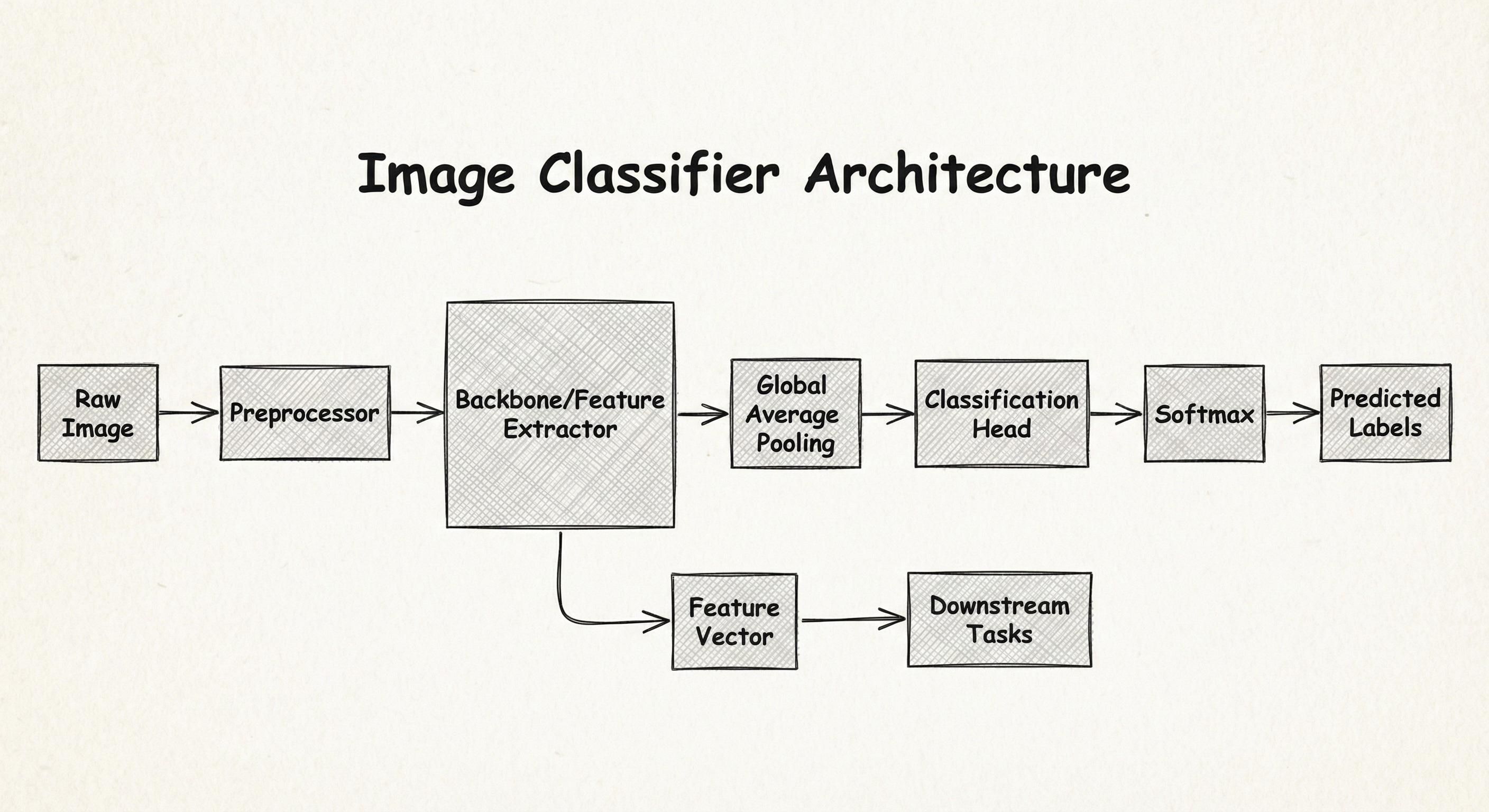
A production image classification system is far more than just the model. It's a pipeline that spans data ingestion, preprocessing, model inference, post-processing, and monitoring. Let's look at the full architecture.
The core model itself follows a backbone + head pattern. The backbone (also called the feature extractor or encoder) processes the raw image through a series of convolutional or attention layers, producing a feature vector. The classification head -- typically a fully connected layer or a small MLP -- maps this feature vector to class logits.
In production, this model sits inside a serving infrastructure that handles batching, GPU scheduling, input validation, output caching, and A/B testing. The preprocessing stage (resizing, normalization, augmentation during training) is critical and must be exactly identical between training and inference -- even a 1-pixel difference in resize interpolation can degrade accuracy.
The backbone architectures in common use today fall into three families:
CNN-based: ResNet, EfficientNet, ConvNeXt, MobileNet. These use convolutional operations that exploit spatial locality and translation invariance. ResNet-50 remains the default baseline due to its well-understood behavior and extensive benchmarking. EfficientNetV2 offers the best accuracy-per-FLOP ratio for most practical workloads. ConvNeXt modernizes ResNet with Transformer-inspired design choices (larger kernels, LayerNorm, GELU activations) and matches ViT performance.
Transformer-based: ViT (Vision Transformer), DeiT, Swin Transformer. These split images into patches and process them with self-attention. ViT-Large achieves state-of-the-art accuracy but requires large datasets (or strong pre-training) and significant compute. Swin Transformer introduces hierarchical feature maps and shifted windows, making it more practical for dense prediction tasks.
Hybrid: CoAtNet, MaxViT, FastViT. These combine convolutional layers (for local feature extraction) with attention layers (for global context). They often achieve the best accuracy-efficiency tradeoffs in practice.
Key Components
Image Preprocessor
Resizes input images to the model's expected resolution (e.g., 224x224 for ResNet, 384x384 for ViT), normalizes pixel values using dataset-specific mean and standard deviation (typically ImageNet statistics: mean=[0.485, 0.456, 0.406], std=[0.229, 0.224, 0.225]), and applies data augmentation during training (random crops, flips, color jitter, RandAugment, Mixup, CutMix).
Backbone / Feature Extractor
The core neural network that transforms raw pixel inputs into a high-dimensional feature representation. This is where the learned feature hierarchy lives -- from low-level edges to high-level semantic concepts. In transfer learning, this component is initialized from pre-trained weights and optionally fine-tuned. Common choices: ResNet-50 (25.6M params), EfficientNet-B4 (19.3M params), ViT-Base/16 (86.6M params).
Global Average Pooling (GAP)
Reduces the spatial dimensions of the backbone's output feature map to a single feature vector by averaging across all spatial positions. For a ResNet-50, this reduces a 7x7x2048 feature map to a 2048-dimensional vector. GAP acts as a regularizer and makes the model invariant to small spatial translations.
Classification Head
A fully connected layer (or small MLP) that maps the pooled feature vector to class logits. For transfer learning, this is the component you always replace and retrain. For a 1000-class ImageNet model adapted to a 10-class problem, this changes from a (2048, 1000) to a (2048, 10) linear layer.
Output Activation
Softmax for multi-class classification (probabilities sum to 1, enforcing mutual exclusivity). Sigmoid for multi-label classification (each class gets an independent probability between 0 and 1). The choice here determines the loss function and evaluation metrics for the entire pipeline.
Post-Processor
Applies confidence thresholds (reject predictions below a threshold), maps model outputs to business labels, handles edge cases (e.g., 'unknown' class for out-of-distribution images), and formats results for downstream consumers. In production, this layer often includes calibration (Platt scaling or temperature scaling) to ensure predicted probabilities are well-calibrated.
Data Flow
Training Path: Raw images are loaded from storage (S3, GCS, or local disk) -> augmented and preprocessed into tensors -> batched (typically 32-256 images per GPU) -> forward pass through backbone and head -> loss computed against ground truth labels -> gradients backpropagated -> optimizer updates weights. This loop repeats for 10-100 epochs depending on dataset size and transfer learning strategy.
Inference Path: A single image (or batch) arrives via API -> preprocessed identically to training (same resize, same normalization, NO augmentation unless using test-time augmentation) -> forward pass through the frozen model -> logits converted to probabilities via softmax/sigmoid -> post-processing (thresholding, label mapping) -> response returned to caller.
Key Invariant: The preprocessing pipeline MUST be identical between training and inference. Any discrepancy -- different interpolation method for resizing, different normalization constants, different image decoding library -- will silently degrade accuracy. This is the single most common deployment bug in image classification systems.
A linear flow from 'Raw Image' through 'Preprocessor', 'Backbone/Feature Extractor', 'Global Average Pooling', 'Classification Head', 'Softmax/Sigmoid' to 'Predicted Labels'. A branch from the backbone outputs a feature vector for downstream tasks like visual search or object detection.
How to Implement
Practical Implementation Strategy
The implementation approach depends on three factors: dataset size, compute budget, and whether a pre-trained model exists for your domain.
Small dataset (<5K images): Use a pre-trained backbone (ResNet-50 or EfficientNet-B0), freeze all backbone layers, and only train the classification head. This is pure transfer learning -- you're using the backbone as a fixed feature extractor. Training takes minutes on a single GPU.
Medium dataset (5K-100K images): Start with a frozen backbone, train the head for 5-10 epochs, then gradually unfreeze backbone layers from top to bottom and fine-tune with a much lower learning rate (10-100x smaller than the head's learning rate). This discriminative fine-tuning strategy preserves low-level features while adapting high-level features to your domain.
Large dataset (>100K images): Fine-tune the entire model end-to-end. You might still benefit from ImageNet pre-training (it converges faster), but the model has enough data to learn domain-specific features at all levels.
Key Implementation Decisions
-
Architecture selection: EfficientNet-B0/B4 for best accuracy-per-FLOP, ResNet-50 for maximum ecosystem support and debugging, ViT-Base for tasks with large datasets and where global context matters, MobileNetV3 for edge/mobile deployment.
-
Optimizer: AdamW with cosine learning rate schedule for Transformers. SGD with momentum (0.9) and step/cosine schedule for CNNs. Learning rate warmup for the first 5-10% of training helps stability.
-
Augmentation strategy: Start with standard augmentations (random crop, horizontal flip, color jitter). Add RandAugment or TrivialAugment for a significant boost with minimal tuning. Mixup and CutMix regularize effectively and help with class imbalance.
-
Mixed precision training: Always use FP16 (or BF16 on A100/H100) mixed precision. It halves memory usage and doubles throughput with negligible accuracy impact. There is no reason not to use it in 2026.
Cost Estimate: Fine-tuning an EfficientNet-B4 on 50K images for 30 epochs takes approximately 2 hours on a single T4 GPU. On AWS, that's roughly 10-15 (~INR 840-1,260).
import torch
import torch.nn as nn
import torchvision.transforms as T
from torchvision.models import efficientnet_b0, EfficientNet_B0_Weights
from torch.utils.data import DataLoader
from torchvision.datasets import ImageFolder

# 1. Define preprocessing (must match training transforms at inference)
train_transforms = T.Compose([
    T.RandomResizedCrop(224),
    T.RandomHorizontalFlip(),
    T.TrivialAugmentWide(),
    T.ToTensor(),
    T.Normalize(mean=[0.485, 0.456, 0.406], std=[0.229, 0.224, 0.225]),
])

val_transforms = T.Compose([
    T.Resize(256),
    T.CenterCrop(224),
    T.ToTensor(),
    T.Normalize(mean=[0.485, 0.456, 0.406], std=[0.229, 0.224, 0.225]),
])

# 2. Load dataset (expects directory structure: root/class_name/image.jpg)
train_dataset = ImageFolder("data/train", transform=train_transforms)
val_dataset = ImageFolder("data/val", transform=val_transforms)
train_loader = DataLoader(train_dataset, batch_size=64, shuffle=True, num_workers=4)
val_loader = DataLoader(val_dataset, batch_size=64, shuffle=False, num_workers=4)

num_classes = len(train_dataset.classes)

# 3. Load pre-trained model and replace classification head
model = efficientnet_b0(weights=EfficientNet_B0_Weights.IMAGENET1K_V1)

# Freeze backbone initially
for param in model.features.parameters():
    param.requires_grad = False

# Replace classifier head
model.classifier = nn.Sequential(
    nn.Dropout(p=0.3),
    nn.Linear(model.classifier[1].in_features, num_classes),
)

device = torch.device("cuda" if torch.cuda.is_available() else "cpu")
model = model.to(device)

# 4. Train head only first
optimizer = torch.optim.AdamW(model.classifier.parameters(), lr=1e-3, weight_decay=0.01)
criterion = nn.CrossEntropyLoss()
scheduler = torch.optim.lr_scheduler.CosineAnnealingLR(optimizer, T_max=10)

for epoch in range(10):
    model.train()
    for images, labels in train_loader:
        images, labels = images.to(device), labels.to(device)
        outputs = model(images)
        loss = criterion(outputs, labels)
        optimizer.zero_grad()
        loss.backward()
        optimizer.step()
    scheduler.step()

# 5. Unfreeze backbone and fine-tune with lower LR
for param in model.features.parameters():
    param.requires_grad = True

optimizer = torch.optim.AdamW([
    {"params": model.features.parameters(), "lr": 1e-5},
    {"params": model.classifier.parameters(), "lr": 1e-4},
], weight_decay=0.01)
scheduler = torch.optim.lr_scheduler.CosineAnnealingLR(optimizer, T_max=20)

for epoch in range(20):
    model.train()
    for images, labels in train_loader:
        images, labels = images.to(device), labels.to(device)
        outputs = model(images)
        loss = criterion(outputs, labels)
        optimizer.zero_grad()
        loss.backward()
        optimizer.step()
    scheduler.step()
This code demonstrates the standard two-phase transfer learning approach for image classification:
Phase 1 (epochs 1-10): Freeze the pre-trained backbone and train only the new classification head. This quickly adapts the output layer to your specific classes without disturbing the learned features.
Phase 2 (epochs 11-30): Unfreeze the entire backbone and fine-tune with discriminative learning rates -- the backbone gets a 10x smaller learning rate (1e-5) than the head (1e-4). This lets the backbone adapt to your domain while preserving the general features learned from ImageNet.
Key details: TrivialAugmentWide provides strong data augmentation with zero hyperparameters to tune. AdamW with cosine annealing is the standard optimizer-scheduler combination. The num_workers=4 in the DataLoader ensures CPU-based data loading doesn't bottleneck GPU training.
import torch
import torch.nn as nn
import torch.nn.functional as F
from torchvision.models import resnet50, ResNet50_Weights


class FocalLoss(nn.Module):
    """Focal Loss for multi-label classification with class imbalance."""
    def __init__(self, alpha=0.25, gamma=2.0):
        super().__init__()
        self.alpha = alpha
        self.gamma = gamma

    def forward(self, logits, targets):
        bce_loss = F.binary_cross_entropy_with_logits(logits, targets, reduction="none")
        probs = torch.sigmoid(logits)
        p_t = probs * targets + (1 - probs) * (1 - targets)
        focal_weight = self.alpha * (1 - p_t) ** self.gamma
        return (focal_weight * bce_loss).mean()


class MultiLabelClassifier(nn.Module):
    """Multi-label image classifier using ResNet-50 backbone."""
    def __init__(self, num_labels: int, pretrained: bool = True):
        super().__init__()
        weights = ResNet50_Weights.IMAGENET1K_V2 if pretrained else None
        backbone = resnet50(weights=weights)
        self.features = nn.Sequential(*list(backbone.children())[:-1])  # Remove FC layer
        self.classifier = nn.Sequential(
            nn.Flatten(),
            nn.Dropout(0.3),
            nn.Linear(2048, 512),
            nn.ReLU(),
            nn.Dropout(0.2),
            nn.Linear(512, num_labels),  # No softmax -- using sigmoid per label
        )

    def forward(self, x):
        features = self.features(x)
        return self.classifier(features)


# Usage
num_labels = 20  # e.g., 20 attributes for a product image
model = MultiLabelClassifier(num_labels=num_labels)
criterion = FocalLoss(alpha=0.25, gamma=2.0)

# Training loop
model.train()
images = torch.randn(16, 3, 224, 224)  # batch of 16 images
targets = torch.randint(0, 2, (16, num_labels)).float()  # multi-hot labels

logits = model(images)
loss = criterion(logits, targets)
loss.backward()

# Inference: apply sigmoid and threshold
model.eval()
with torch.no_grad():
    logits = model(images)
    probs = torch.sigmoid(logits)
    predictions = (probs > 0.5).int()  # threshold at 0.5
This example illustrates two critical concepts:
-
Multi-label classification architecture: Unlike multi-class (softmax), each label gets an independent sigmoid activation. The model outputs raw logits, and we apply
sigmoid+ thresholding at inference time. This allows an image to have zero, one, or many labels simultaneously -- essential for tasks like product attribute prediction (a shirt can be both "blue" and "cotton" and "formal"). -
Focal Loss for class imbalance: In real-world multi-label datasets, most labels are absent for most images (the target matrix is sparse). Standard BCE loss wastes gradient on easy negatives. Focal loss with down-weights these easy examples by a factor of , focusing training on the hard cases that actually improve the model.
import onnxruntime as ort
import numpy as np
from PIL import Image
from typing import List, Dict
import json


class ImageClassifierService:
    """Production image classifier with ONNX Runtime for fast inference."""

    def __init__(self, model_path: str, labels_path: str, input_size: int = 224):
        self.session = ort.InferenceSession(
            model_path,
            providers=["CUDAExecutionProvider", "CPUExecutionProvider"],
        )
        self.input_name = self.session.get_inputs()[0].name
        self.input_size = input_size
        with open(labels_path) as f:
            self.labels = json.load(f)

        # ImageNet normalization constants
        self.mean = np.array([0.485, 0.456, 0.406], dtype=np.float32).reshape(1, 3, 1, 1)
        self.std = np.array([0.229, 0.224, 0.225], dtype=np.float32).reshape(1, 3, 1, 1)

    def preprocess(self, image: Image.Image) -> np.ndarray:
        image = image.convert("RGB").resize(
            (self.input_size, self.input_size), Image.BILINEAR
        )
        arr = np.array(image, dtype=np.float32) / 255.0
        arr = arr.transpose(2, 0, 1)  # HWC -> CHW
        arr = (arr - self.mean[0]) / self.std[0]
        return arr

    def predict_batch(self, images: List[Image.Image], top_k: int = 5) -> List[Dict]:
        batch = np.stack([self.preprocess(img) for img in images])
        logits = self.session.run(None, {self.input_name: batch})[0]

        # Softmax
        exp_logits = np.exp(logits - logits.max(axis=1, keepdims=True))
        probs = exp_logits / exp_logits.sum(axis=1, keepdims=True)

        results = []
        for prob in probs:
            top_indices = prob.argsort()[-top_k:][::-1]
            results.append({
                "predictions": [
                    {"label": self.labels[str(idx)], "confidence": float(prob[idx])}
                    for idx in top_indices
                ]
            })
        return results


# Usage
service = ImageClassifierService("model.onnx", "labels.json")
images = [Image.open(f"test_{i}.jpg") for i in range(8)]
results = service.predict_batch(images, top_k=3)
This production-ready inference service demonstrates several best practices:
- ONNX Runtime for deployment: exporting the PyTorch model to ONNX and serving with ONNX Runtime typically gives 2-4x speedup over native PyTorch inference, and decouples the serving framework from the training framework.
- Batched inference: processing multiple images in a single forward pass maximizes GPU utilization. On a T4, batch size 8 is often 3-4x faster than processing images one at a time.
- Numerically stable softmax: subtracting the max logit before exponentiation prevents overflow.
- Provider fallback:
CUDAExecutionProviderfor GPU, falling back to CPU if GPU is unavailable. This makes the service portable across deployment environments.
# Training configuration (YAML)
model:
  backbone: efficientnet_b4
  pretrained: imagenet
  num_classes: 150
  dropout: 0.3
  head: linear  # or mlp

data:
  train_dir: data/train
  val_dir: data/val
  input_size: 380
  batch_size: 32
  num_workers: 8
  augmentation:
    - RandomResizedCrop: {size: 380, scale: [0.7, 1.0]}
    - RandomHorizontalFlip: {p: 0.5}
    - TrivialAugmentWide: {}
    - Normalize: {mean: [0.485, 0.456, 0.406], std: [0.229, 0.224, 0.225]}

training:
  epochs: 30
  optimizer: adamw
  learning_rate: 1e-3
  weight_decay: 0.01
  scheduler: cosine
  warmup_epochs: 3
  mixed_precision: true
  gradient_clip: 1.0
  label_smoothing: 0.1

  # Two-phase fine-tuning
  freeze_backbone_epochs: 5
  backbone_lr_multiplier: 0.1

loss:
  type: focal  # or cross_entropy
  focal_gamma: 2.0
  focal_alpha: 0.25

evaluation:
  metrics: [accuracy, top5_accuracy, f1_macro, per_class_f1]
  best_metric: f1_macro
  early_stopping_patience: 7
Common Implementation Mistakes
- ●
Training-inference preprocessing mismatch: Using different resize interpolation (bilinear vs. bicubic), different normalization constants, or different image decoding libraries (PIL vs. OpenCV decode RGB differently) between training and serving. This silently drops accuracy by 2-10%. Always serialize your preprocessing pipeline alongside the model.
- ●
Not using pre-trained weights: Training from scratch on a dataset smaller than 100K images almost always underperforms transfer learning. Even for highly specialized domains (satellite imagery, medical X-rays), ImageNet pre-training provides a better starting point than random initialization.
- ●
Using softmax for multi-label problems: Softmax enforces mutual exclusivity -- probabilities sum to 1. If an image can have multiple labels (e.g., a dish that is both 'spicy' and 'vegetarian'), you need sigmoid activations with binary cross-entropy, not softmax with categorical cross-entropy.
- ●
Ignoring class imbalance: Real-world datasets are almost never balanced. A defect detection dataset might be 99% 'normal' and 1% 'defective'. Training with standard cross-entropy will produce a model that always predicts 'normal' with 99% accuracy -- and misses every defect. Use focal loss, class-weighted loss, or resampling strategies.
- ●
Skipping learning rate warmup: Especially with pre-trained models, starting with a high learning rate can destroy the pre-trained features in the first few iterations. Use linear warmup for 5-10% of total training steps before applying the main schedule.
- ●
Overfitting to augmentation: Applying excessive augmentation (extreme rotations, heavy color distortion) on small datasets can cause the model to learn augmentation artifacts rather than genuine visual features. Start with mild augmentation and increase gradually while monitoring validation loss.
- ●
Not monitoring per-class metrics: Overall accuracy can mask poor performance on minority classes. Always track precision, recall, and F1 per class. A model with 95% overall accuracy might have 0% recall on a rare but critical class.
When Should You Use This?
Use When
You need to assign categorical labels to images -- the canonical image classification task (product categorization, content moderation, medical diagnosis, quality inspection)
Your problem has a well-defined, relatively stable set of classes (tens to low thousands of categories)
Sufficient labeled training data exists or can be collected (at least 100-500 images per class for transfer learning)
You need a feature extraction backbone for downstream tasks like object detection, similarity search, or visual recommendation
Inference latency requirements are in the 10-100ms range (achievable with optimized CNN/ViT models on GPU or even CPU)
The visual patterns that distinguish classes are learnable from 2D images (texture, shape, color, spatial relationships)
You want to leverage the massive ecosystem of pre-trained models, tooling, and research built around image classification
Avoid When
You need to locate objects within images (use object detection or segmentation instead -- though the classifier backbone is often shared)
Your label space is open-ended or changes frequently (consider CLIP-based zero-shot classification or a retrieval-based approach instead)
You have fewer than 50-100 labeled examples per class and cannot collect more -- few-shot learning or zero-shot approaches may be more appropriate
The task requires understanding spatial relationships between objects (use scene graph generation or visual question answering)
The input is video and temporal dynamics matter (use video classification architectures like TimeSformer or SlowFast)
Simple rule-based heuristics (color thresholding, template matching) can solve the problem -- don't use a neural network where OpenCV suffices
Key Tradeoffs
Accuracy vs. Latency vs. Cost
This is the central tradeoff triangle for image classifiers in production. Here's a concrete comparison:
| Model | Top-1 Acc (ImageNet) | Params | GFLOPs | Latency (T4, batch=1) | Training Cost (50K images, 30 epochs) |
|---|---|---|---|---|---|
| MobileNetV3-Large | 75.2% | 5.4M | 0.22 | ~3ms | ~INR 15 ($0.18) |
| EfficientNet-B0 | 77.1% | 5.3M | 0.39 | ~5ms | ~INR 25 ($0.30) |
| ResNet-50 | 80.4% | 25.6M | 4.1 | ~8ms | ~INR 45 ($0.54) |
| EfficientNet-B4 | 82.9% | 19.3M | 4.5 | ~12ms | ~INR 90 ($1.08) |
| ConvNeXt-Base | 83.8% | 88.6M | 15.4 | ~18ms | ~INR 180 ($2.16) |
| ViT-Base/16 | 81.8% | 86.6M | 17.6 | ~15ms | ~INR 250 ($3.00) |
| ViT-Large/16 | 82.5% | 304.3M | 61.6 | ~45ms | ~INR 840 ($10.08) |
CNN vs. Transformer: When to Choose Which
Choose CNNs (EfficientNet, ConvNeXt) when: your dataset is small-to-medium (<100K images), you need fast inference on edge devices, your compute budget is limited, or you need well-understood, debuggable architectures.
Choose Transformers (ViT, Swin) when: you have a large dataset (>500K images) or strong pre-training, you need to capture global context (the entire image matters, not just local patterns), or you plan to use the same backbone for multiple vision tasks (ViT backbones transfer well to detection and segmentation).
Choose Hybrid models (CoAtNet, FastViT) when: you want the best of both worlds -- local feature extraction from convolutions and global context from attention -- and your latency budget is moderate.
Transfer Learning vs. Training from Scratch
Transfer learning almost always wins. Even when your domain looks nothing like ImageNet (medical images, satellite imagery, microscopy), the low-level features (edges, textures) learned from ImageNet transfer well. The only exception is when your images are fundamentally different in structure -- e.g., spectrograms, radar images, or highly stylized graphics where natural image statistics don't apply.
Rule of Thumb: Start with EfficientNet-B0 + transfer learning. It's the Toyota Camry of image classification -- not the flashiest, but reliable, efficient, and gets the job done. Upgrade to B4 or ConvNeXt-Base only if accuracy demands it and your latency budget allows.
Alternatives & Comparisons
Object detectors (YOLO, Faster R-CNN) classify AND localize objects within images. If you only need to know what's in the image (not where), an image classifier is simpler, faster, and more accurate. If you need bounding boxes or per-object labels, use an object detector -- but note that most detectors use a classifier backbone internally.
Feature extraction produces a dense embedding vector for similarity search rather than discrete class labels. Use feature extraction when the goal is retrieval or similarity ("find images like this one") rather than categorization ("this image is a cat"). In practice, the classifier backbone often serves double duty: classification head for labeling, feature vector (from the penultimate layer) for retrieval.
The image preprocessor handles resizing, normalization, and augmentation before the classifier sees the image. It's not an alternative but an essential upstream component. A well-designed preprocessor can be worth 2-5% accuracy improvement through proper augmentation, while a mismatched preprocessor between training and inference can silently destroy performance.
The model training pipeline is the infrastructure (data loading, distributed training, experiment tracking, hyperparameter tuning) that trains the image classifier. The classifier is the model; the training pipeline is the factory that produces it. At scale, the training pipeline becomes more complex than the model itself.
Pros, Cons & Tradeoffs
Advantages
Mature ecosystem: Decades of research, hundreds of pre-trained models, battle-tested frameworks (PyTorch, TensorFlow), and comprehensive tooling. You're never starting from zero.
Transfer learning dramatically reduces data requirements: With ImageNet pre-training, you can achieve strong performance with as few as 100-500 images per class, compared to the thousands needed when training from scratch.
Efficient inference: Optimized models (MobileNetV3, EfficientNet-B0) can run at 3-5ms per image on a T4 GPU, or even on mobile CPUs at 30-50ms. This makes real-time classification feasible even on budget hardware.
Versatile backbone: The same feature extractor trained for classification can be repurposed for object detection (Faster R-CNN), segmentation (U-Net), visual search (embedding extraction), and more. One training investment, many downstream applications.
Well-understood failure modes: Unlike newer paradigms (generative models, multimodal systems), image classifiers have well-documented failure modes and established debugging techniques. Confusion matrices, GradCAM visualizations, and per-class metrics make diagnosis straightforward.
Scalable serving: Classifier models compress well (quantization, pruning, distillation) and batch efficiently on GPUs. A single T4 instance (~INR 28/hour on AWS) can serve 500+ inferences per second.
Disadvantages
Requires labeled training data: Every class needs sufficient labeled examples. Labeling is expensive -- at INR 1-3 per image annotation via services like Labelbox or Scale AI, a 100K-image dataset costs INR 1-3 lakh (3,600).
Closed-world assumption: The model can only predict classes it was trained on. Novel classes require retraining. This is problematic for rapidly evolving catalogs (e-commerce, content moderation where new violation types emerge).
Sensitive to distribution shift: A model trained on studio-quality product photos will fail on user-uploaded images with poor lighting, motion blur, or unusual angles. Robustness to distribution shift requires careful augmentation and periodic retraining.
Class imbalance is pervasive: Real-world class distributions are almost never uniform. A Flipkart catalog has millions of "t-shirts" but only hundreds of "antique gramophones". Handling this requires specialized loss functions, sampling strategies, and evaluation metrics.
Black-box predictions: Despite interpretability techniques (GradCAM, SHAP), it can be difficult to explain WHY a model made a specific prediction. This is a regulatory concern in medical imaging and financial applications.
Computational cost scales with accuracy: The jump from 80% to 85% accuracy might require a 10x larger model and 50x more training data. Diminishing returns are steep at the high end.
Failure Modes & Debugging
Training-inference preprocessing skew
Cause
Different image decoding libraries (PIL vs. OpenCV), different resize interpolation methods (bilinear vs. bicubic), or different normalization constants between training and serving. This is the most common and most insidious failure in production classifiers.
Symptoms
Accuracy on the production serving system is consistently 2-10% lower than reported during offline evaluation, despite using the exact same model weights. The gap is unexplained by data distribution differences.
Mitigation
Serialize the preprocessing pipeline as part of the model artifact (e.g., include transforms in the ONNX graph or use torchvision.transforms consistently). Write integration tests that compare preprocessing outputs between training and serving environments. Use a shared preprocessing library.
Class imbalance collapse
Cause
Heavily imbalanced class distribution (e.g., 95% of images are class A, 5% across classes B-F) causes the model to learn to always predict the majority class, achieving high overall accuracy while completely failing on minority classes.
Symptoms
High overall accuracy (e.g., 95%) but near-zero recall on minority classes. The confusion matrix shows the model never predicts certain classes. Users report the model 'doesn't work' for specific categories.
Mitigation
Use focal loss () or class-weighted cross-entropy. Apply oversampling (duplicate minority samples) or undersampling (reduce majority samples). Use Mixup/CutMix augmentation which naturally smooths class boundaries. Evaluate with macro-averaged F1 instead of overall accuracy. Set up per-class recall alerts.
Distribution shift / domain gap
Cause
Training data distribution differs from production data. Common scenarios: model trained on curated studio images but deployed on user-uploaded photos; model trained on one camera sensor but deployed on another; seasonal/temporal drift in visual patterns.
Symptoms
Accuracy degrades gradually over time. The model performs well on the validation set but poorly on live traffic. GradCAM shows the model attending to irrelevant features (background instead of the object).
Mitigation
Implement continuous monitoring of prediction confidence distributions and per-class accuracy. Set up a data flywheel: sample low-confidence predictions for human labeling and periodically retrain. Use domain randomization and aggressive augmentation during training to improve robustness.
Adversarial / out-of-distribution inputs
Cause
The model receives images entirely outside its training distribution -- blank images, screenshots, memes, or adversarially crafted inputs. Since softmax always produces a probability distribution, the model will confidently classify even random noise into some category.
Symptoms
High-confidence predictions on nonsensical inputs. Users exploit the classifier by uploading adversarial images. The system fails silently without raising errors.
Mitigation
Add an OOD (out-of-distribution) detection layer: monitor the maximum softmax probability and flag inputs below a confidence threshold (e.g., 0.7). Train a binary 'in-distribution vs. out-of-distribution' classifier. Use Monte Carlo Dropout at inference time to estimate prediction uncertainty.
Label noise corruption
Cause
Training labels contain errors -- human annotators made mistakes, automated labeling pipelines introduced systematic errors, or ambiguous edge cases were inconsistently labeled. At scale (Zomato labels 100K images daily), even a 5% label error rate means 5,000 incorrect labels per day.
Symptoms
Model accuracy plateaus below expected levels despite sufficient data. The model learns to reproduce labeling errors. Per-class confusion matrix shows systematic confusion between visually similar classes that were likely mislabeled.
Mitigation
Use label cleaning techniques: train a model, identify samples where the model's prediction consistently disagrees with the label (these are likely mislabeled), and send them for re-annotation. Libraries like cleanlab automate this process. Implement label smoothing () to reduce the model's sensitivity to label noise.
Catastrophic forgetting during fine-tuning
Cause
When fine-tuning a pre-trained model with a high learning rate or without proper scheduling, the model 'forgets' the useful features learned during pre-training and overfits to the (often small) fine-tuning dataset.
Symptoms
Training loss decreases rapidly but validation loss increases after a few epochs. The fine-tuned model performs worse than a model with a frozen backbone. Feature visualizations show the model has lost its ability to detect basic visual patterns.
Mitigation
Use discriminative learning rates: 10-100x smaller LR for early backbone layers compared to the classification head. Apply gradual unfreezing: train the head first (5-10 epochs), then unfreeze layers progressively from top to bottom. Use weight decay (0.01-0.1) and early stopping on validation loss.
Placement in an ML System
Where Does the Image Classifier Sit?
In a computer vision pipeline, the image classifier sits right after the preprocessor and represents the first stage of visual understanding. Its outputs feed into two main downstream paths:
-
Direct classification output: The predicted class label drives business logic -- routing a customer support ticket with an attached image, flagging inappropriate content, categorizing a product listing on Flipkart, or triaging a medical scan.
-
Feature backbone for downstream tasks: The classifier's penultimate layer outputs serve as rich visual features for object detection (the ResNet-50 backbone in Faster R-CNN), visual search (extracting embeddings for similarity retrieval), and image segmentation (encoder in U-Net or DeepLab).
In a recommendation system (like Myntra's style recommendations), the classifier identifies product attributes (color, pattern, style) that feed into the recommendation engine. The classifier is one signal among many, but it provides structured visual features that complement collaborative filtering.
In a content moderation pipeline (like ShareChat or Moj), the classifier runs on every uploaded image, classifying it across multiple moderation dimensions (NSFW, violence, hate speech in text overlays). This is a multi-label classification task where recall on harmful content is prioritized over precision.
Key Insight: The image classifier is both a standalone component and a feature factory. Its backbone provides the visual understanding that powers most other computer vision tasks in the system.
Pipeline Stage
Inference / Serving
Upstream
- image-preprocessor
- model-training
Downstream
- object-detector
- feature-extraction
Scaling Bottlenecks
The primary bottleneck is GPU compute at inference time. A single T4 GPU can handle approximately 300-500 inferences per second for EfficientNet-B0 at batch size 32. For a platform like Swiggy processing millions of food images daily, this translates to needing 2-4 GPU instances during peak hours.
Image decoding and preprocessing can become CPU-bound. Decoding a JPEG image takes 2-5ms on CPU, which can dominate the total latency for lightweight models. Libraries like nvJPEG (GPU-accelerated JPEG decoding) or pre-decoded image caches can help.
Model size and memory scale with the number of classes. A ResNet-50 classifier with 10 classes takes ~100 MB. The same backbone with 10,000 classes takes ~180 MB due to the larger classification head. This is rarely a bottleneck for classification but matters when the same backbone serves multiple tasks.
Data labeling and retraining is the operational bottleneck. As new classes are added or the data distribution shifts, the classifier needs retraining. Automating the data flywheel -- collecting low-confidence predictions, sending them for labeling, retraining, validating, and deploying -- is the key scalability challenge for the ML team.
Some concrete cost numbers: serving an EfficientNet-B4 classifier at 100 QPS with P99 latency < 50ms requires approximately one T4 GPU instance. On AWS (g4dn.xlarge), that costs ~$0.526/hour or roughly INR 1,300/day (~INR 39,000/month). On E2E Networks (India), equivalent GPU instances start around INR 22,000/month.
Production Case Studies
Official AWS Machine Learning blog post co-authored by Zomato ML engineers, detailing their computer vision system that uses CNNs to classify 500M+ images into categories (food, ambiance, menu, human) and digitize restaurant menus at scale.
Processes 100,000 new images daily; menu digitization system uses Amazon Textract and SageMaker with 4,086 labeled images costing $1,400 for annotation, enabling automatic dish-based restaurant recommendations.
Pinterest evolved their visual search system through progressively advanced classifier architectures -- from AlexNet (2014) to VGG16 to ResNet/ResNeXt (2016) to SE-ResNeXt (2018). The classifier backbone powers their Pinterest Lens feature, which processes over 150 million visual searches per month. They train visual embeddings with a proxy-based metric learning approach, using the classification backbone as the feature extractor.
Pinterest Lens enables real-time visual search across billions of Pins, with the classifier backbone providing the visual understanding that matches user photos to similar products and ideas. The system has driven significant increases in shopping engagement on the platform.
Swiggy built a Food Intelligence platform using deep learning classifiers to categorize food items into a structured taxonomy. Their multi-label classification system assigns cuisine type, dish category, and dietary attributes to each menu item using image and text features. They use an encoder-decoder architecture with a ResNet encoder and transformer decoder for ingredient prediction from food images, enabling automated menu understanding at scale.
Automated food categorization across millions of menu items from 200,000+ restaurant partners. The system enables personalized food recommendations, search improvements, and operational optimizations like predicting preparation time based on dish complexity.
Google's Cloud Vision API provides image classification as a managed service, powered by models trained on Google's massive internal image datasets. The API classifies images into thousands of categories (label detection), detects explicit content (SafeSearch), identifies landmarks, and reads text. Under the hood, it uses an ensemble of EfficientNet and ViT models with multi-task learning across all these capabilities.
Serves millions of classification requests daily across industries. Customers like Disney, Realtor.com, and The New York Times use the API for content organization, moderation, and visual search. Pricing at $1.50 per 1,000 images (~INR 126 per 1,000 images) makes it accessible for teams that don't want to train custom models.
OLX, a global online classifieds platform, built a visual fraud detection system using triplet loss training to identify stolen product photos. Fraudsters commonly steal photos from legitimate listings to create fake ads. OLX trained a CNN with triplet loss to learn image embeddings where identical/near-identical images cluster together, enabling near-duplicate detection at marketplace scale across millions of listings (2020).
The triplet loss-based image classifier detects 95%+ of stolen photos with minimal false positives, significantly reducing fraudulent listings. The system processes new listing images in real-time, comparing against the entire existing catalog to flag suspected fraud before listings go live.
Tooling & Ecosystem
The dominant framework for image classification research and production. torchvision.models provides 50+ pre-trained classifier architectures (ResNet, EfficientNet, ViT, ConvNeXt, MobileNet, etc.) with standardized APIs. Supports mixed precision training, distributed training, and export to ONNX/TorchScript.
The largest collection of PyTorch image classification models: 1,000+ architectures with pre-trained weights. Created by Ross Wightman and now maintained by Hugging Face. Includes ResNet, EfficientNet, ViT, Swin, ConvNeXt, MaxViT, and many more. The go-to library when torchvision doesn't have the architecture you need.
Hugging Face's Transformers library supports ViT, Swin, DeiT, BEiT, and other transformer-based classifiers with a unified API. Includes Trainer for fine-tuning, pipeline for quick inference, and seamless integration with the Hugging Face Hub for model sharing.
High-performance inference engine for deploying trained classifiers. Supports CPU, GPU (CUDA, TensorRT), and edge devices. Typically provides 2-4x speedup over native PyTorch inference. Essential for production serving where every millisecond counts.
Google's ML framework with built-in tf.keras.applications providing pre-trained classifiers (EfficientNet, ResNet, MobileNet, etc.). Strong support for TFLite (mobile/edge deployment) and TensorFlow Serving (production serving). Still widely used in production systems at Indian companies like Google India, Flipkart, and Jio.
Fast image augmentation library that supports 70+ augmentation techniques. Optimized for speed (uses OpenCV under the hood) and commonly used in production training pipelines. Supports spatial transforms (crops, rotations), pixel transforms (color jitter, blur), and advanced techniques (GridDistortion, CoarseDropout).
Experiment tracking and visualization platform widely used for image classification projects. Log training metrics, compare runs, visualize predictions, and track model versions. Integrates with PyTorch, TensorFlow, and Keras out of the box. Free tier available for individual researchers.
Automated data quality and label error detection library. Uses confident learning to identify mislabeled images in training datasets. Critical for large-scale classification where manual label verification is infeasible. Can improve accuracy by 2-5% simply by fixing label errors.
Research & References
He, Zhang, Ren & Sun (2016)CVPR 2016
Introduced ResNet with skip connections, enabling training of networks with 152+ layers. Solved the vanishing gradient problem and remains the most widely-used classifier backbone. ResNet-50 is still the default baseline for image classification benchmarks.
Tan & Le (2019)ICML 2019
Proposed compound scaling -- uniformly scaling network depth, width, and resolution with a fixed ratio. EfficientNet-B7 achieved 84.3% top-1 accuracy on ImageNet while being 8.4x smaller than the best existing CNN. The EfficientNet family remains the go-to for accuracy-efficient classification.
Dosovitskiy, Beyer, Kolesnikov et al. (2021)ICLR 2021
Introduced the Vision Transformer (ViT), proving that pure Transformer architectures (without convolutions) can match or exceed CNN performance on image classification when pre-trained on large datasets. Spawned an entire family of vision transformer variants.
Liu, Mao, Wu et al. (2022)CVPR 2022
Introduced ConvNeXt, a pure CNN that modernizes ResNet with Transformer-inspired design choices (patchify stem, inverted bottleneck, larger kernels, LayerNorm, GELU). Matched Swin Transformer accuracy while maintaining CNN simplicity, proving that CNNs still have untapped potential.
Lin, Goyal, Girshick, He & Dollar (2017)ICCV 2017
Introduced focal loss to address extreme class imbalance by down-weighting easy examples. While designed for object detection (RetinaNet), focal loss has become the standard loss function for imbalanced classification tasks across all domains.
Tan & Le (2021)ICML 2021
Improved on the original EfficientNet with Fused-MBConv blocks and progressive learning (increasing image size during training). EfficientNetV2-L achieves 85.7% top-1 on ImageNet while training 5-11x faster than the original EfficientNet.
Liu, Lin, Cao et al. (2021)ICCV 2021 (Best Paper)
Introduced shifted window self-attention, enabling linear computational complexity with respect to image size (vs. quadratic for ViT). Produces hierarchical feature maps suitable for dense prediction tasks. Won ICCV 2021 Best Paper and became the standard backbone for detection and segmentation.
Northcutt, Jiang & Chuang (2021)Journal of Artificial Intelligence Research (JAIR)
Formalized the problem of label noise in datasets and introduced confident learning to identify and correct mislabeled examples. The associated cleanlab library has become essential for improving training data quality in production classification systems.
Interview & Evaluation Perspective
Common Interview Questions
- ●
Design an image classification system for Flipkart to categorize 10 million product images into 5,000 categories. Walk me through architecture, training, and deployment.
- ●
How would you handle severe class imbalance in a defect detection classifier where only 1% of images contain defects?
- ●
Explain the tradeoffs between ResNet-50, EfficientNet-B4, and ViT-Base for a production image classifier. When would you choose each?
- ●
What is transfer learning, and why does it work so well for image classification? When might it fail?
- ●
How do you ensure consistency between your training preprocessing pipeline and your production inference pipeline?
- ●
Design a multi-label image classification system for content moderation that handles NSFW, violence, and hate speech detection.
- ●
Your image classifier's accuracy dropped 5% after deployment. Walk me through your debugging process.
Key Points to Mention
- ●
Always start with transfer learning from ImageNet (or better, ImageNet-21K). Training from scratch is almost never the right choice unless your domain is fundamentally different from natural images.
- ●
Architecture selection is a function of constraints: EfficientNet-B0 for latency-constrained serving, ResNet-50 for maximum ecosystem compatibility, ViT for large datasets where global context matters, MobileNetV3 for edge deployment.
- ●
Multi-class vs. multi-label changes everything: loss function (CE vs. BCE), activation (softmax vs. sigmoid), evaluation metric (accuracy vs. mAP), and serving logic. Clarify this requirement upfront.
- ●
Preprocessing parity between training and inference is the #1 deployment pitfall. Serialize transforms with the model artifact and write integration tests.
- ●
Class imbalance is the norm, not the exception. Always check the class distribution before training. Use focal loss, class-weighted loss, or oversampling. Evaluate with macro-F1, not overall accuracy.
- ●
Monitoring in production: track prediction confidence distribution, per-class accuracy drift, input data distribution shifts, and latency P99. Set up automated retraining triggers.
Pitfalls to Avoid
- ●
Claiming you would train a CNN from scratch on a 10K-image dataset -- this immediately signals you don't understand transfer learning.
- ●
Proposing only 'overall accuracy' as the evaluation metric without considering class imbalance, per-class metrics, or top-k accuracy.
- ●
Ignoring the preprocessing pipeline when discussing deployment -- this is where most production bugs live.
- ●
Not discussing the cost implications: a ViT-Large might give 2% higher accuracy, but at 10x the inference cost. Always frame architecture choices in terms of the accuracy-latency-cost tradeoff.
- ●
Forgetting to mention data augmentation -- it's often worth 3-5% accuracy improvement and is essentially free at training time.
- ●
Treating image classification as a solved one-time task rather than a continuous system that requires monitoring, retraining, and label maintenance.
Senior-Level Expectation
A senior/staff-level candidate should discuss the full system lifecycle, not just the model. This includes: data pipeline design (labeling strategy, active learning, label quality assurance with tools like cleanlab), training infrastructure (distributed training, experiment tracking, hyperparameter search), model selection with quantitative justification (FLOPs, latency, accuracy tradeoffs), deployment strategy (model optimization with ONNX/TensorRT, A/B testing, canary deployments), monitoring (data drift detection, per-class accuracy tracking, confidence calibration), and the organizational process (how to handle escalations when the model fails, when to retrain vs. add training data vs. change the architecture). The candidate should naturally discuss cost optimization -- for instance, using T4 GPUs for inference instead of A100s, or quantizing the model to INT8 for a 2x latency reduction with <1% accuracy drop. At Indian startups, compute budget awareness separates senior from mid-level engineers.
Summary
Let's recap what we've covered about image classification in ML systems:
An image classifier maps input images to categorical labels using a learned feature hierarchy. The modern approach is overwhelmingly transfer learning: take a backbone pre-trained on ImageNet (ResNet-50, EfficientNet, ViT, ConvNeXt), replace the classification head, and fine-tune on your domain-specific data. This approach reduces data requirements by 10-100x and training time by a similar factor. The choice of backbone depends on your constraints: EfficientNet-B0/B4 for the best accuracy-per-FLOP, MobileNetV3 for edge deployment, ViT for large datasets with global context, and ResNet-50 when you need maximum ecosystem support and debuggability.
The critical design decisions are: multi-class vs. multi-label (softmax + CE vs. sigmoid + BCE -- get this wrong and everything downstream breaks), class imbalance handling (focal loss, class-weighted loss, oversampling -- real-world datasets are never balanced), and preprocessing parity (training and inference must use identical transforms -- this is the #1 source of production bugs). For serving, export to ONNX and use ONNX Runtime or TensorRT for 2-4x speedup over native PyTorch. A single T4 GPU (~INR 20,000/month) can serve 500+ inferences/second for EfficientNet-B0.
The image classifier is both a standalone component and a feature factory. Its backbone provides the visual understanding that powers object detection, segmentation, visual search, and content moderation. Master the fundamentals here -- architecture selection, transfer learning, class imbalance, augmentation strategy, and deployment optimization -- and you have the foundation for the entire computer vision stack in any ML system.