Normalization in Machine Learning
Normalization is the unglamorous workhorse of every ML pipeline -- the preprocessing step that rescales your raw feature values into a common range or distribution so that downstream models can actually learn from them. Skip it and your gradient descent will zigzag like an autorickshaw in Bengaluru traffic; get it right and your model converges faster, generalizes better, and produces stable predictions.
At its core, normalization addresses a fundamental mismatch: raw features come in wildly different scales. A user's age might range from 18 to 80, their annual income from 200,000 to 50,000,000 (in INR), and a sensor reading from 0.001 to 0.999. Without normalization, any distance-based or gradient-based algorithm will be dominated by the high-magnitude feature -- income will drown out everything else.
This guide covers the three classical normalization techniques (min-max, Z-score, and decimal scaling), extends into L1/L2 vector normalization, draws the critical boundary between data-level normalization and deep-learning normalization layers (BatchNorm, LayerNorm), and provides production-ready code you can drop into a scikit-learn or TensorFlow pipeline today.
Whether you are building a fraud detection model at Razorpay, a recommendation engine at Flipkart, or a demand forecasting system at Swiggy, understanding when and how to normalize your features is non-negotiable. Let's dig in.
Concept Snapshot
- What It Is
- A data preprocessing technique that transforms numerical features to a common scale or distribution without distorting relative differences between values.
- Category
- Data Processing
- Complexity
- Beginner
- Inputs / Outputs
- Inputs: raw numerical feature vectors with arbitrary ranges and distributions. Outputs: rescaled feature vectors in a standardized range (e.g., [0,1]) or distribution (e.g., mean 0, variance 1).
- System Placement
- Sits after data cleaning and before feature extraction or model training in a typical ML pipeline. Applied during preprocessing, carried forward into serving via saved scaler parameters.
- Also Known As
- feature scaling, data scaling, feature normalization, data standardization, range scaling, variance scaling
- Typical Users
- ML Engineers, Data Scientists, Data Analysts, MLOps Engineers, Research Scientists
- Prerequisites
- Basic statistics (mean, standard deviation, variance), Understanding of feature vectors and tabular data, Familiarity with gradient descent optimization, Basic Python / NumPy
- Key Terms
- min-max scalingZ-score standardizationdecimal scalingL1 normL2 normunit variancefeature rangetraining-serving skewscaler parametersrobust scaling
Why This Concept Exists
The Scale Mismatch Problem
Imagine you are building a loan default prediction model at a fintech company like Razorpay. Your feature set includes:
- Age: 21 to 65
- Annual income: INR 1,80,000 to INR 5,00,00,000 (~600,000)
- Credit score: 300 to 900
- Loan amount: INR 50,000 to INR 1,00,00,000 (~120,000)
- Number of existing loans: 0 to 15
Without normalization, a gradient-based model sees income as 10,000x more important than age simply because its numerical range is 10,000x larger. The gradient update for the income weight will dominate every other weight, causing the optimizer to oscillate wildly along the income dimension while barely moving along the others. The result? Slow convergence, poor generalization, or outright training failure.
Why Not Just Let the Model Figure It Out?
Tree-based models (Random Forests, XGBoost, LightGBM) are largely immune to feature scale differences because they split on rank order, not magnitude. But the moment you use any of the following, normalization becomes critical:
- Linear regression / logistic regression: Coefficients are directly proportional to feature scale
- Support Vector Machines (SVMs): Kernel computations depend on distances between feature vectors
- K-Nearest Neighbors (KNN): Euclidean distance is scale-sensitive
- Neural networks: Gradient descent is sensitive to input scale, and unnormalized inputs cause exploding or vanishing activations
- K-Means clustering: Centroid computation uses Euclidean distance
- Principal Component Analysis (PCA): Variance-based, so high-scale features dominate principal components
Historical Evolution
Normalization is not a modern invention. Statistical standardization (Z-score) dates back to the early 20th century, introduced as part of the standard normal distribution framework. Min-max scaling became popular with early neural network research in the 1980s and 1990s, where sigmoid activations required inputs in the [0,1] range to avoid saturation.
The modern era brought two key developments. First, scikit-learn (released 2007) made normalization trivially easy with its fit/transform API, establishing the pattern of learning scaler parameters from training data and applying them consistently to test/production data. Second, Ioffe and Szegedy's 2015 Batch Normalization paper showed that normalization could happen inside the network itself, not just as a preprocessing step -- a breakthrough that enabled training of much deeper networks.
Today, normalization is a first-class concern in production ML platforms. Google's TFX Transform component, Uber's Michelangelo Palette, and Feature Store systems all include normalization as a core transformation primitive, ensuring consistency between training and serving.
Key Takeaway: Normalization exists because raw features live on incompatible scales. Without it, distance-based and gradient-based algorithms cannot function correctly. It is one of the simplest yet most impactful steps in the entire ML pipeline.
Core Intuition & Mental Model
The Mental Model: Units of Measurement
Here is the simplest way to think about normalization: it is a unit conversion for your features. If you are comparing distances between cities, you would not mix kilometers and miles in the same calculation. Similarly, you should not mix features measured in INR (lakhs) with features measured in years or counts without converting them to a common "unit."
Normalization does not change the information content of your features -- it changes the scale so that every feature gets a fair vote in the model's decision-making process. A normalized income of 0.75 and a normalized age of 0.75 contribute equally to a distance calculation, whereas raw income of 37,50,000 would completely overwhelm raw age of 45.
Three Flavors, One Goal
Think of the three classical normalization methods as three different ways to standardize a ruler:
-
Min-Max Normalization says: "Let the smallest value be 0, the largest be 1, and everything else proportionally in between." Simple, bounded, and intuitive -- like resizing a photograph to fit a frame.
-
Z-Score Standardization says: "Let the average value be 0, and measure everything in units of standard deviation." This is the statistical purist's approach -- it tells you how many standard deviations a value is from the mean, regardless of the original scale.
-
Decimal Scaling says: "Divide everything by a power of 10 so the largest absolute value is less than 1." Quick and dirty -- useful when you need a fast approximation and don't want to compute full statistics.
Each method has different properties when it comes to outliers, bounded ranges, and distributional assumptions. The right choice depends on your data and your model -- and we will cover that decision framework in detail.
The Gradient Descent Connection
Why does normalization make gradient descent converge faster? Picture the loss landscape as a topographic map. When features are on different scales, the contours of the loss surface become highly elongated ellipses -- the gradient points away from the minimum and the optimizer bounces between the walls of a narrow valley. After normalization, the contours become more circular, and the gradient points much more directly toward the minimum. Fewer steps, less oscillation, faster convergence. This is not just theory -- it is the single most common reason training runs fail or take 10x longer than expected.
Technical Foundations
Min-Max Normalization
Min-max normalization rescales each feature to a target range , most commonly :
For the default range , this simplifies to:
Properties:
- Output is bounded in
- Preserves the shape of the original distribution
- Sensitive to outliers: a single extreme value compresses all other values into a narrow sub-range
- Time complexity: per feature (single pass to find min/max, single pass to transform)
Z-Score Standardization
Z-score standardization transforms each feature to have zero mean and unit variance:
where is the sample mean and is the sample standard deviation.
Properties:
- Output is unbounded (no fixed range)
- Resulting distribution has and
- More robust to outliers than min-max (outliers do not compress the range of non-outlier values)
- Assumes features are approximately Gaussian for optimal behavior (but works reasonably well even when they are not)
- Time complexity: per feature (two passes: one for statistics, one for transform)
Decimal Scaling Normalization
Decimal scaling normalizes by dividing each value by a power of 10 such that the maximum absolute value becomes less than 1:
where is the smallest integer such that .
Properties:
- Output range is
- Preserves sign and relative ordering
- Extremely fast: only requires finding the maximum absolute value
- Less commonly used in practice because it does not center or standardize the distribution
- Time complexity: per feature
L1 Normalization (Manhattan Norm)
L1 normalization scales each sample (row) so that the absolute values of its components sum to 1:
This projects each sample onto the L1 unit ball (a diamond/rhombus shape in 2D).
L2 Normalization (Euclidean Norm)
L2 normalization scales each sample so that it lies on the unit hypersphere:
This is critical for cosine similarity calculations, where vectors must be unit-normalized for the dot product to equal the cosine of the angle between them.
Batch Normalization (Deep Learning)
Batch normalization normalizes activations within a mini-batch during training:
where and are the mini-batch mean and variance, is a small constant for numerical stability, and , are learned affine parameters.
Critical Distinction: Min-max, Z-score, and decimal scaling operate on features (columns) across samples. L1/L2 normalization operates on samples (rows) across features. Batch normalization operates on activations within a neural network layer. These are three fundamentally different axes of normalization.
Internal Architecture
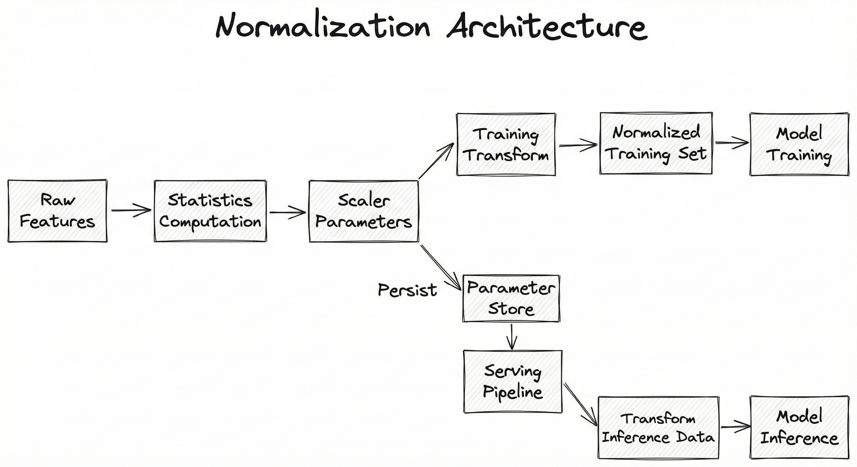
The normalization pipeline in a production ML system is deceptively simple in concept but requires careful engineering to avoid training-serving skew. The architecture consists of three stages: statistics computation (learning the scaler parameters), transformation (applying the normalization), and parameter persistence (saving and loading scaler state for serving).
In a typical setup, the statistics computation runs once on the training data during the training pipeline. The computed parameters (min, max, mean, standard deviation, or power-of-10 exponent) are serialized and stored alongside the model artifact. At serving time, the same parameters are loaded and applied to incoming feature vectors before they reach the model -- ensuring that the normalization applied during inference is identical to what was applied during training.
The critical architectural invariant is: scaler parameters must be computed ONLY from training data and applied identically to validation, test, and production data. Computing statistics on the full dataset (including test data) introduces data leakage, and using different statistics at serving time causes training-serving skew -- both of which silently degrade model performance.
Key Components
Statistics Analyzer
Computes aggregate statistics from the training data: per-feature min, max, mean, standard deviation, or maximum absolute value depending on the chosen normalization method. Runs as a single full pass over the training dataset.
Scaler Transformer
Applies the normalization formula to each feature vector using the pre-computed statistics. Operates element-wise, transforming raw values into normalized values. Must be deterministic and invertible (for debugging and interpretability).
Parameter Store
Serializes and persists the scaler parameters (e.g., as a pickle file, JSON, or part of a TFX Transform SavedModel). Ensures the same parameters are available at both training and serving time. In production, this is often a versioned artifact in a model registry.
Pipeline Integration Layer
Wraps the scaler into the broader ML pipeline using abstractions like sklearn.pipeline.Pipeline, TFX Transform, or a Feature Store transformation. Ensures normalization is applied consistently and in the correct order relative to other preprocessing steps (e.g., after imputation but before feature selection).
Inverse Transformer
Reverses the normalization to recover original-scale values. Essential for model interpretability, SHAP explanations, and debugging predictions. Supported by inverse_transform() in scikit-learn scalers.
Data Flow
Training Path: Raw feature vectors flow from the data store into the Statistics Analyzer, which computes and caches normalization parameters. These parameters feed into the Scaler Transformer, which outputs normalized feature vectors to the model training loop. Parameters are simultaneously written to the Parameter Store for later retrieval.
Serving Path: Incoming feature vectors at inference time are intercepted by the Pipeline Integration Layer, which loads the saved scaler parameters from the Parameter Store and applies the identical transformation before passing the normalized vectors to the model. This ensures zero training-serving skew.
Monitoring Path: A monitoring sidecar compares the distribution of incoming features against the training distribution statistics. If the incoming feature range drifts significantly beyond the scaler's learned min/max or mean/std, a data drift alert is triggered -- indicating the scaler parameters may need recomputation.
A directed flow diagram showing Raw Features flowing into a Statistics Computation stage that outputs Scaler Parameters. These parameters feed both the Training Transform path (producing normalized training data for model training) and the Serving Transform path (normalizing inference data for model prediction). The scaler parameters are persisted to a Parameter Store that bridges the training and serving pipelines.
How to Implement
Practical Implementation Approaches
Normalization implementation falls into three tiers of complexity:
Tier 1: Standalone scikit-learn scalers. Perfect for offline batch training, prototyping, and Kaggle competitions. You fit() on training data, transform() train/test data, and pickle the scaler for later use. This covers 80% of use cases.
Tier 2: Pipeline-integrated normalization. Using sklearn.pipeline.Pipeline or sklearn.compose.ColumnTransformer, you embed the scaler into the model pipeline itself. This eliminates the possibility of forgetting to normalize at serving time, because the pipeline object includes both the scaler and the model.
Tier 3: Production-grade normalization. Using TFX Transform, Feature Store transformations (Feast, Tecton), or custom serving code. This is where you handle streaming features, versioned scaler parameters, data drift detection, and the full lifecycle of scaler management. Companies like Google (TFX), Uber (Michelangelo Palette), and Razorpay (Apache Flink-based pipelines) operate at this tier.
The key principle across all tiers is the same: learn statistics from training data only, apply everywhere consistently. The implementation details change, but this invariant does not.
Cost Consideration: For most Indian startups, Tier 1 or Tier 2 is sufficient. Moving to Tier 3 typically costs INR 5-15 lakh/year (~18,000/year) in engineering time and infrastructure, and is only justified when you have multiple models sharing features across real-time serving endpoints.
import numpy as np

# Feature 0: Age | Feature 1: Income INR | Feature 2: Credit score
X = np.array([
    [25, 350000, 720], [45, 1200000, 650],
    [32, 580000, 810], [55, 4500000, 430], [28, 290000, 780],
], dtype=np.float64)

# --- Min-Max Normalization [0, 1] ---
def min_max_normalize(X_train):
    x_min, x_max = X_train.min(axis=0), X_train.max(axis=0)
    return (X_train - x_min) / (x_max - x_min), (x_min, x_max)

# --- Z-Score Standardization ---
def z_score_normalize(X_train):
    mu, sigma = X_train.mean(axis=0), X_train.std(axis=0)
    return (X_train - mu) / sigma, (mu, sigma)

# --- Decimal Scaling ---
def decimal_scaling(X_train):
    max_abs = np.abs(X_train).max(axis=0)
    j = np.ceil(np.log10(max_abs + 1e-10)).astype(int)
    divisor = 10.0 ** j
    return X_train / divisor, divisor

X_mm, _ = min_max_normalize(X)
X_zs, _ = z_score_normalize(X)
X_ds, _ = decimal_scaling(X)
print("Min-Max:", X_mm[0])   # [0.0, 0.014, 0.763]
print("Z-Score:", X_zs[0])   # [-0.86, -0.64, 0.53]
print("Decimal:", X_ds[0])   # [0.25, 0.035, 0.72]
All three classical normalization methods implemented from scratch. The decimal_scaling function calculates the smallest power of 10 that makes the max absolute value less than 1. Note: always compute statistics from training data only; apply the saved parameters to test/production data. For production use, prefer scikit-learn's optimized implementations.
from sklearn.pipeline import Pipeline
from sklearn.compose import ColumnTransformer
from sklearn.preprocessing import StandardScaler, RobustScaler, MinMaxScaler
from sklearn.linear_model import LogisticRegression
from sklearn.model_selection import train_test_split
import pandas as pd, numpy as np, joblib

np.random.seed(42)
n = 10000
df = pd.DataFrame({
    "age": np.random.randint(21, 65, n),
    "income_inr": np.random.lognormal(13, 1, n).astype(int),
    "credit_score": np.random.randint(300, 900, n),
    "loan_amount_inr": np.random.lognormal(12, 0.8, n).astype(int),
    "num_existing_loans": np.random.randint(0, 10, n),
    "default": np.random.binomial(1, 0.15, n),
})

X = df.drop("default", axis=1)
y = df["default"]
X_train, X_test, y_train, y_test = train_test_split(
    X, y, test_size=0.2, random_state=42, stratify=y
)

preprocessor = ColumnTransformer(transformers=[
    ("zscore", StandardScaler(), ["age", "credit_score"]),
    ("robust", RobustScaler(), ["income_inr", "loan_amount_inr"]),
    ("minmax", MinMaxScaler(), ["num_existing_loans"]),
])

pipe = Pipeline([
    ("preprocessor", preprocessor),
    ("classifier", LogisticRegression(max_iter=1000)),
])
pipe.fit(X_train, y_train)
print(f"Test accuracy: {pipe.score(X_test, y_test):.4f}")
joblib.dump(pipe, "loan_default_pipeline.joblib")
# Serving: pipe = joblib.load(...); pipe.predict(new_data)
This is the production-recommended pattern. By wrapping the scaler inside a ColumnTransformer within a Pipeline, you achieve several goals: (1) different features get different normalization strategies, (2) the scaler parameters are learned exclusively from training data, (3) the entire pipeline is serializable as a single artifact, and (4) normalization is automatically applied at prediction time. Note the use of RobustScaler for income and loan amount, which are typically right-skewed with outliers -- using the IQR instead of mean/std prevents a few high-income individuals from distorting the scaling.
from sklearn.preprocessing import normalize
import numpy as np

# Sample feature vectors (e.g., TF-IDF or raw embeddings)
X = np.array([
    [3.0, 4.0, 0.0],
    [1.0, 1.0, 1.0],
    [0.0, 0.0, 5.0],
])

# L2 normalization: each row becomes a unit vector
X_l2 = normalize(X, norm="l2")
print("L2 norms per row:", np.linalg.norm(X_l2, axis=1))
# Output: [1.0, 1.0, 1.0]

# L1 normalization: absolute values per row sum to 1
X_l1 = normalize(X, norm="l1")
print("L1 norms per row:", np.abs(X_l1).sum(axis=1))
# Output: [1.0, 1.0, 1.0]

# Why this matters: cosine similarity between L2-normalized vectors
# equals their dot product -- no need for the full cosine formula
from numpy import dot
cos_sim = dot(X_l2[0], X_l2[1])
print(f"Cosine similarity (via dot product): {cos_sim:.4f}")
L1/L2 normalization operates row-wise (per sample), unlike min-max and Z-score which operate column-wise (per feature). L2 normalization is essential when you need cosine similarity -- after L2 normalization, the dot product between any two vectors directly equals their cosine similarity, which is a major computational shortcut used in vector stores and recommendation systems. L1 normalization is useful for sparse data like TF-IDF vectors, where you want each document's feature weights to sum to 1.
import tensorflow as tf
from tensorflow.keras import layers, Model
import numpy as np

# --- Option 1: tf.keras.layers.Normalization (data-level) ---
# Learns mean/variance from training data, applies at inference
norm_layer = layers.Normalization(axis=-1)

# Adapt (fit) on training data
X_train = np.random.randn(1000, 5).astype(np.float32)
X_train[:, 0] *= 1000  # Scale feature 0 to a large range
norm_layer.adapt(X_train)

# Build model with normalization as first layer
model = tf.keras.Sequential([
    norm_layer,
    layers.Dense(64, activation="relu"),
    layers.Dense(1, activation="sigmoid"),
])

model.compile(optimizer="adam", loss="binary_crossentropy")
print("Normalization mean:", norm_layer.mean.numpy()[:3])
print("Normalization variance:", norm_layer.variance.numpy()[:3])

# --- Option 2: Batch Normalization (activation-level) ---
# Normalizes activations per mini-batch during training,
# uses running statistics during inference
model_with_bn = tf.keras.Sequential([
    layers.Dense(128),
    layers.BatchNormalization(),  # normalizes after dense, before activation
    layers.Activation("relu"),
    layers.Dense(64),
    layers.BatchNormalization(),
    layers.Activation("relu"),
    layers.Dense(1, activation="sigmoid"),
])

model_with_bn.compile(optimizer="adam", loss="binary_crossentropy")
print(f"\nBatchNorm model params: {model_with_bn.count_params()}")
This example shows the two fundamentally different places normalization happens in deep learning. layers.Normalization is data-level normalization -- it learns mean/variance from training data via adapt() and applies Z-score standardization to inputs. layers.BatchNormalization is activation-level normalization -- it normalizes intermediate activations within the network during training. Both serve normalization goals but at different stages: data normalization handles the input, batch normalization handles the internal representations. In production, you typically use BOTH.
import tensorflow as tf
import tensorflow_transform as tft

# This function runs inside a TFX Transform component
# It defines feature transformations that are consistent
# between training and serving
def preprocessing_fn(inputs):
    outputs = {}

    # Z-score normalization using full training set statistics
    outputs["age_normalized"] = tft.scale_to_z_score(
        inputs["age"]
    )

    # Min-Max scaling to [0, 1]
    outputs["credit_score_scaled"] = tft.scale_to_0_1(
        inputs["credit_score"]
    )

    # Log transform + Z-score for heavily skewed features
    outputs["income_normalized"] = tft.scale_to_z_score(
        tf.math.log1p(tf.cast(inputs["income_inr"], tf.float32))
    )

    # Bucketize + one-hot (alternative to normalization)
    outputs["age_bucket"] = tft.bucketize(
        inputs["age"], num_buckets=5
    )

    # Pass through label unchanged
    outputs["label"] = inputs["label"]

    return outputs

# The key advantage: TFX generates a TF SavedModel that
# encodes these transforms, so the exact same normalization
# is applied during serving with zero code duplication.
TFX Transform is Google's production solution for normalization (and other feature transformations). The preprocessing_fn defines transformations declaratively -- TFX analyzes the full training dataset to compute statistics (mean, std, min, max) and then generates a TensorFlow graph that applies these transforms. The resulting SavedModel is deployed alongside the trained model, guaranteeing zero training-serving skew. Note the combination of log1p with scale_to_z_score for the income feature -- this is a common pattern for right-skewed monetary features in Indian financial datasets where incomes can span orders of magnitude.
# sklearn pipeline config (YAML representation)
pipeline:
  steps:
    - name: preprocessor
      type: ColumnTransformer
      transformers:
        - name: numeric_zscore
          scaler: StandardScaler
          columns: ["age", "credit_score", "tenure_months"]
        - name: numeric_minmax
          scaler: MinMaxScaler
          feature_range: [0, 1]
          columns: ["num_transactions"]
        - name: monetary_robust
          scaler: RobustScaler
          quantile_range: [25.0, 75.0]
          columns: ["income_inr", "loan_amount_inr"]
    - name: model
      type: LogisticRegression
      params:
        max_iter: 1000
        C: 0.1

# Scaler persistence
artifact_store:
  path: s3://ml-artifacts/scalers/
  versioning: enabled
  format: joblib
Common Implementation Mistakes
- ●
Fitting the scaler on the entire dataset (including test data): This is the most common and most harmful mistake. When you compute min/max or mean/std from the full dataset, information from the test set leaks into the training process, inflating evaluation metrics and producing models that perform worse in production than on your test set. Always call
fit()on training data only, thentransform()on train, validation, test, and production data. - ●
Normalizing the target variable unintentionally: For regression tasks, normalizing the target (y) can be useful for training stability, but you MUST remember to inverse-transform predictions back to the original scale. Forgetting this step results in predictions that are meaningless (e.g., predicting a house price of 0.73 instead of INR 73,00,000).
- ●
Applying column-wise normalization when row-wise is needed (or vice versa): Min-max and Z-score normalize features across samples (column-wise). L1/L2 normalize samples across features (row-wise). Confusing these axes produces completely wrong results. If you are working with TF-IDF vectors or embeddings that need cosine similarity, you need row-wise L2 normalization, not column-wise standardization.
- ●
Ignoring the impact of outliers on min-max scaling: A single extreme value (e.g., an income of INR 100 crore in a dataset where most incomes are under INR 50 lakh) will compress 99.9% of your data into a tiny fraction of the [0,1] range. Use
RobustScaleror clip outliers before applying min-max scaling. - ●
Not persisting scaler parameters for serving: Training a great model with normalized features but then serving it with raw features (or with scaler parameters computed from a different data slice) introduces training-serving skew. Always serialize the scaler alongside the model artifact.
- ●
Normalizing categorical features: One-hot encoded or label-encoded categorical variables should NOT be normalized. Normalizing a binary indicator (0/1) to have mean 0 and std 1 is mathematically valid but semantically meaningless and can hurt tree-based models that rely on exact split values.
When Should You Use This?
Use When
Your model uses gradient descent optimization (neural networks, logistic regression, SVMs) and features are on different scales -- normalization is almost always required here
You are computing distances or similarities between samples (KNN, K-Means, cosine similarity in recommendation/search systems)
Features have vastly different ranges (e.g., age 18-65 vs. income INR 1.8L-5Cr) and you want each feature to contribute proportionally
You are using PCA or other variance-based dimensionality reduction techniques where high-scale features would dominate
Your neural network activations are saturating (sigmoid/tanh outputs clustering at 0 or 1) due to large input magnitudes
You want faster convergence during training -- normalization can reduce required training epochs by 2-10x
You are deploying models behind a feature store and need consistent, versioned transformations across training and serving
Avoid When
You are using tree-based models exclusively (Random Forest, XGBoost, LightGBM, CatBoost) -- these are invariant to monotonic feature transformations, so normalization adds complexity with zero benefit
Your features are already on the same scale (e.g., all are percentages between 0-100, or all are boolean indicators)
You are working with count data that will be fed into Poisson regression or other count-based models that expect raw counts
Your feature engineering specifically relies on absolute magnitudes (e.g., a rule-based system that triggers when transaction amount exceeds INR 10,00,000)
You are using algorithms that internally normalize (some implementations of Naive Bayes, certain kernel methods)
The feature is categorical, ordinal, or already one-hot encoded -- normalizing these distorts their semantics
Key Tradeoffs
Min-Max vs. Z-Score: The Central Decision
| Criterion | Min-Max | Z-Score |
|---|---|---|
| Output range | Bounded [0, 1] | Unbounded |
| Outlier sensitivity | High (compresses non-outliers) | Moderate (outliers get extreme z-scores but don't compress others) |
| Distribution assumption | None | Works best with approximately Gaussian data |
| Best for | Neural networks with sigmoid/tanh, image pixel values, algorithms needing bounded inputs | Linear models, PCA, SVM, any algorithm assuming centered data |
| Information preserved | Relative distances within the observed range | Statistical properties (mean, variance) |
When to Use Robust Scaling
If your data has significant outliers (common in Indian financial datasets -- think a few INR 100Cr+ transactions in a pool of INR 10,000-10,00,000 transactions), RobustScaler using the IQR is your best bet. It scales based on the median and interquartile range, making it immune to extreme values. The tradeoff is that it does not bound the output range.
The Hidden Cost of Normalization
Normalization adds operational complexity. Every scaler introduces state (its learned parameters) that must be versioned, persisted, and kept in sync between training and serving. For a pipeline with 50 features using 3 different scalers, that is 3 serialized scaler objects, each coupled to the training data distribution. When your data distribution drifts (and it will), you need to decide whether to retrain the scalers -- and that means retraining the model too.
Rule of Thumb: Start with
StandardScaler(Z-score) as the default. Switch toMinMaxScalerif you need bounded outputs. Switch toRobustScalerif outliers are a problem. UseNormalizer(L2) only when you need unit-norm sample vectors. And always, always persist your scaler parameters.
Alternatives & Comparisons
Normalization is a specific subset of feature scaling. The broader scaling category includes log transforms, Box-Cox transforms, Yeo-Johnson transforms, and quantile transforms. When your feature distribution is heavily skewed (e.g., income, transaction amounts in INR), a log or Box-Cox transform followed by Z-score standardization often outperforms raw Z-score alone. Use general feature scaling when distribution shape matters more than range.
Data cleaning handles missing values, duplicates, and data quality issues. Normalization handles scale differences. They are complementary: always clean first, then normalize. Applying normalization to dirty data (e.g., features with missing values encoded as -999) produces misleading results. Data cleaning is upstream of normalization in every well-designed pipeline.
Feature extraction creates new features from raw data (e.g., TF-IDF from text, embeddings from images). Normalization rescales existing features. The two often work together: you extract features, then normalize them before feeding to a model. Some extraction methods (like TF-IDF) produce inherently scaled outputs, reducing the need for additional normalization.
Data transformation is a broader category that includes normalization, encoding, binning, polynomial features, and more. Normalization is specifically about rescaling numerical features to a common range or distribution. Use data transformation when you need structural changes to your features (e.g., one-hot encoding, log transforms, interaction terms) beyond simple rescaling.
Pros, Cons & Tradeoffs
Advantages
Dramatically faster gradient descent convergence -- normalization can reduce training time by 2-10x by transforming the loss landscape from elongated ellipses to near-circular contours, letting the optimizer take more direct paths to the minimum
Equal feature contribution -- ensures no single high-magnitude feature dominates distance calculations or gradient updates, giving all features a fair influence on model predictions regardless of their original measurement unit
Improved numerical stability -- prevents floating-point overflow or underflow in computations involving features with extreme ranges (e.g., multiplying INR 50,000,000 by a small weight can cause precision issues)
Better model interpretability -- with Z-score normalization, feature coefficients in linear models become directly comparable: a coefficient of 0.5 for age and 0.3 for income means age genuinely has more predictive power, not just a larger scale
Enables effective regularization -- L1/L2 regularization penalizes coefficient magnitude; without normalization, the regularizer disproportionately penalizes features with small scales, effectively imposing different regularization strengths per feature
Compatible with transfer learning and pretrained models -- many pretrained models expect inputs in specific ranges (e.g., ImageNet models expect pixel values normalized to mean=[0.485, 0.456, 0.406], std=[0.229, 0.224, 0.225])
Disadvantages
Adds operational complexity -- every scaler introduces state that must be versioned, persisted, and kept in sync between training and serving; this is a real maintenance burden at scale
Sensitive to training data distribution -- scaler parameters are only as good as the training data they were computed from; if production data drifts (new feature ranges, different distributions), the normalization becomes stale and can degrade performance
Outliers can distort scaling -- a single extreme value in the training set (e.g., a billionaire in a dataset of middle-class incomes) can compress the useful range of min-max scaling to a tiny fraction of [0,1]
Loss of absolute magnitude information -- after normalization, you lose the ability to reason about raw feature values (e.g., "income above INR 10 lakh") without inverse-transforming, which complicates debugging and business rule integration
Training-serving skew risk -- if the scaler applied during serving differs even slightly from the one used during training (different version, different data slice, rounding differences), model predictions silently degrade
Not universally needed -- applying normalization to tree-based models adds pipeline complexity with zero benefit, and normalizing categorical/binary features is actively harmful
Failure Modes & Debugging
Data Leakage Through Full-Dataset Fitting
Cause
Calling scaler.fit(X) on the entire dataset (including test/validation data) before splitting, or calling fit_transform() on the full dataset. This is the most common normalization bug in data science code.
Symptoms
Inflated test/validation metrics that do not reproduce in production. The model appears to perform well offline but underperforms when deployed. The gap between offline and online metrics is the telltale sign.
Mitigation
Always split data first, then fit the scaler exclusively on the training split. Use sklearn.pipeline.Pipeline to enforce this automatically. In code reviews, grep for fit_transform applied before train_test_split -- this pattern is almost always a bug.
Training-Serving Skew from Mismatched Scaler Parameters
Cause
Serving infrastructure loads a different version of the scaler than the one used during training, or computes normalization statistics from a different data source. Common when scaler artifacts are not versioned alongside model artifacts.
Symptoms
Model predictions are systematically biased or have higher variance than expected. Input feature distributions at serving time do not match the expected normalized distribution. Prediction confidence scores may cluster at extremes.
Mitigation
Bundle the scaler into the same artifact as the model (e.g., a single Pipeline object in scikit-learn, or a single SavedModel in TFX). Version the combined artifact in your model registry. Add a serving-time validation check that compares the scaler's expected input statistics against actual incoming feature distributions.
Outlier-Induced Range Compression
Cause
Applying MinMaxScaler to features with extreme outliers. For example, if income ranges from INR 2,00,000 to INR 100,00,00,000 but 99% of values are below INR 50,00,000, the [0,1] range is dominated by the single outlier, and 99% of values are squeezed into [0, 0.005].
Symptoms
Most normalized values cluster near 0 (or near 1 if the outlier is at the low end). The model effectively treats the feature as nearly constant for the majority of samples, destroying its predictive power.
Mitigation
Use RobustScaler (IQR-based) instead of MinMaxScaler for outlier-prone features. Alternatively, clip outliers before normalization using percentile-based bounds (e.g., clip at 1st and 99th percentile). For monetary features in Indian datasets, a log transform before normalization is often the best approach.
Zero Variance Feature Division by Zero
Cause
Applying Z-score standardization to a feature with zero variance (all values are identical). The standard deviation is 0, causing a division-by-zero error or NaN values.
Symptoms
NaN or Inf values in the normalized dataset, which propagate through the model and produce NaN losses or predictions. Some implementations silently return 0, masking the issue.
Mitigation
Add a variance check before normalization: drop or flag features with near-zero variance (e.g., sklearn.feature_selection.VarianceThreshold). Scikit-learn's StandardScaler handles this gracefully by leaving zero-variance features unchanged, but custom implementations may not.
Distribution Shift Rendering Scaler Parameters Stale
Cause
The production data distribution shifts over time (concept drift or data drift), but the scaler parameters remain fixed from the original training data. For example, a salary prediction model trained in 2023 with mean income INR 8,00,000 encounters 2026 data where mean income is INR 12,00,000 due to inflation.
Symptoms
Normalized feature values systematically shift (e.g., more values above 1.0 for min-max, or the Z-score distribution is no longer centered at 0). Model performance degrades gradually over weeks or months.
Mitigation
Implement data drift monitoring that compares incoming feature distributions against the training distribution. Set alerts when the Kolmogorov-Smirnov statistic or Population Stability Index (PSI) exceeds a threshold. Retrain the scaler (and model) on a regular cadence or when drift is detected.
Incorrect Normalization Axis (Column vs. Row)
Cause
Applying column-wise normalization (Z-score, min-max) when row-wise normalization (L1, L2) is needed, or vice versa. This is common when switching between tabular data (column-wise) and text/embedding data (row-wise).
Symptoms
For column-wise error on embeddings: cosine similarity calculations produce incorrect rankings. For row-wise error on tabular data: features lose their individual statistical properties and become meaningless.
Mitigation
Explicitly document the normalization axis in your pipeline code. Use sklearn.preprocessing.StandardScaler (column-wise) vs. sklearn.preprocessing.Normalizer (row-wise) -- the API makes the distinction clear. In code reviews, always verify which axis is being normalized.
Placement in an ML System
Where Normalization Fits in the ML Pipeline
Normalization sits in the data processing / feature engineering stage, after raw data has been cleaned (missing values handled, duplicates removed, outliers identified) and after basic feature extraction (e.g., converting timestamps to day-of-week, extracting text length). It is typically the last transformation before features enter the model.
In a production pipeline at a company like Razorpay or Zerodha, the flow looks like this:
- Data ingestion (Kafka, event streams) -> 2. Data cleaning (null handling, deduplication) -> 3. Feature extraction (aggregations, encodings) -> 4. Normalization (scaling to model-expected ranges) -> 5. Model training / inference
The normalization step acts as a contract between the feature engineering pipeline and the model: the model expects inputs in a specific distribution (e.g., zero mean, unit variance), and the normalization step guarantees that contract is met. Breaking this contract -- by changing the scaler, retraining on different data, or simply forgetting to normalize at serving time -- is one of the most common causes of silent model degradation in production.
Key Insight: Think of normalization as the "adapter" between your data and your model. The data speaks in raw units (INR, years, counts); the model speaks in normalized units. The scaler is the translator, and it must be the same translator at training and serving time.
Pipeline Stage
Data Processing / Feature Engineering
Upstream
- data-cleaning
- feature-extraction
- data-transformation
Downstream
- model-training
- feature-extraction
- scaling
Scaling Bottlenecks
Normalization itself is computationally cheap -- where is the number of samples and is the number of features. For a dataset with 100 million rows and 500 features, a single-threaded Python implementation takes roughly 30-60 seconds; with NumPy vectorization, it drops to 2-5 seconds.
The real bottleneck is not the transformation but the statistics computation on the full training set. For distributed training (e.g., Spark MLlib, Dask, Ray), computing global mean/std across partitioned data requires a reduce step that introduces communication overhead. At Flipkart or Swiggy scale (billions of events per day), this statistics computation may itself need to be distributed.
Another scaling concern is scaler parameter management. With hundreds of models, each potentially using different scaler configurations for different feature sets, the number of scaler artifacts that need to be versioned, stored, and served grows combinatorially. Feature stores (Feast, Tecton, Hopsworks) address this by centralizing feature transformations.
Production Case Studies
Google's Machine Learning Crash Course explicitly recommends normalization as a core preprocessing step. Their TFX Transform component (tft.scale_to_z_score, tft.scale_to_0_1) provides production-grade normalization that generates a TensorFlow SavedModel encoding the exact transformation -- ensuring zero training-serving skew. This pattern is used internally across Google's ML infrastructure for Search ranking, Ads prediction, and YouTube recommendations.
TFX Transform processes billions of examples per day across Google's ML pipelines. The key insight is that baking normalization into the model graph eliminates an entire class of training-serving skew bugs.
Uber's Michelangelo ML platform includes a feature transformation DSL that supports normalization and bucketization. Features like ride distance (0.5 to 200 km), surge multiplier (1.0 to 8.0), and estimated fare (500) are normalized before feeding into pricing and ETA prediction models. Michelangelo Palette (their feature store) ensures that the same normalization is applied in both batch training and real-time serving.
Michelangelo serves predictions for millions of rides per day. Centralized feature normalization through Palette reduced feature-related production incidents by standardizing transformations across hundreds of ML models.
Razorpay's ML team uses Apache Flink for real-time feature engineering including normalization of transaction features for fraud detection models. Transaction amounts (ranging from INR 1 to INR 10,00,00,000+), merchant risk scores, and velocity features are normalized using robust scaling techniques to handle the extreme skew typical of Indian payment data. The real-time pipeline ensures normalized features are available within milliseconds for serving.
Real-time normalized features enabled Razorpay to detect fraudulent transactions with sub-100ms latency at their scale of processing millions of transactions daily, while maintaining consistent feature distributions between model training and live serving.
Netflix's recommendation system normalizes diverse user interaction signals -- watch time (0 to 180 minutes), scroll depth, thumbs-up/down counts, and recency features -- into comparable scales before feeding them into their ranking models. Their engineering team has published extensively on the importance of consistent feature preprocessing for maintaining recommendation quality across their 260M+ subscriber base.
Netflix attributes approximately 80% of content viewed to recommendations powered by their ML systems. Proper feature normalization is a foundational requirement for combining heterogeneous user signals into a single ranking score.
Tooling & Ecosystem
The gold standard for tabular data normalization. Provides StandardScaler (Z-score), MinMaxScaler (min-max), RobustScaler (IQR-based), MaxAbsScaler, Normalizer (L1/L2 row-wise), PowerTransformer (Box-Cox/Yeo-Johnson), and QuantileTransformer. All follow the fit/transform API and integrate with Pipeline for safe, leak-free preprocessing.
Google's production library for feature preprocessing in TFX pipelines. Functions like tft.scale_to_z_score() and tft.scale_to_0_1() analyze the full dataset, compute statistics, and produce a TensorFlow graph that applies the exact transformation at serving time. Eliminates training-serving skew by design.
PyTorch provides nn.BatchNorm1d/2d/3d, nn.LayerNorm, nn.GroupNorm, and nn.InstanceNorm as built-in normalization layers for deep learning. These handle activation-level normalization within neural networks, complementing data-level normalization applied to inputs.
For quick normalization without scikit-learn, NumPy's vectorized operations (np.mean, np.std, np.min, np.max) and pandas' built-in methods (df.apply, broadcasting) provide a lightweight alternative. Common in EDA notebooks and Kaggle kernels.
Distributed normalization for big data. Spark MLlib's StandardScaler and MinMaxScaler compute statistics across a Spark DataFrame distributed across a cluster, enabling normalization of datasets too large to fit in memory on a single machine. Used at companies like Flipkart and Swiggy for batch feature engineering.
Open-source feature store that supports feature transformations including normalization. By defining normalization as a feature transformation in Feast, you ensure the same scaling is applied consistently across online serving, offline training, and batch scoring. Integrates with scikit-learn and pandas transformations.
Research & References
Ioffe, S. & Szegedy, C. (2015)ICML 2015
The foundational paper introducing batch normalization as a technique for normalizing activations within neural network layers. Showed that BatchNorm enables higher learning rates, reduces sensitivity to initialization, and acts as a regularizer -- fundamentally changing how deep networks are trained.
Ba, J. L., Kiros, J. R. & Hinton, G. E. (2016)arXiv preprint (widely cited, 10,000+ citations)
Proposed LayerNorm as an alternative to BatchNorm that normalizes across features within a single sample rather than across the batch. Now the standard normalization in Transformer architectures (GPT, BERT, LLaMA) where batch statistics are impractical.
Wu, Y. & He, K. (2018)ECCV 2018
Introduced GroupNorm, which divides channels into groups and normalizes within each group. Achieved 10.6% lower error than BatchNorm on ImageNet with batch size 2, making it the preferred choice for GPU-memory-constrained training and detection/segmentation tasks.
Patro, S. G. & Sahu, K. K. (2015)arXiv preprint
A systematic review of classical normalization techniques including min-max, Z-score, and decimal scaling. Provides formal definitions, comparative analysis, and proposes integer scaling as an additional technique. Widely cited as a reference for data preprocessing fundamentals.
Wu, S., Li, G., Deng, L., Liu, L., Wu, D., Xie, Y. & Shi, L. (2018)arXiv preprint
Proposed replacing L2-norm-based batch normalization with L1-norm, which avoids costly square and square-root operations. L1BN achieves nearly identical accuracy to standard BatchNorm while being computationally cheaper -- important for edge deployment in cost-sensitive markets.
Baier-Reinio, A. & Xu, L. (2024)arXiv preprint
A 2024 deep-dive into the geometric properties of LayerNorm, proving its irreversibility property and comparing it with RMSNorm (used in LLaMA models). Provides modern theoretical grounding for why normalization layers work in Transformers.
Interview & Evaluation Perspective
Common Interview Questions
- ●
When should you normalize features and when should you not? Give specific examples.
- ●
What is the difference between normalization and standardization?
- ●
How does feature normalization affect gradient descent convergence? Explain geometrically.
- ●
You have a feature with extreme outliers (e.g., income in India ranging from INR 50,000 to INR 100 Crore). How would you normalize it?
- ●
What happens if you fit the scaler on the entire dataset before splitting into train/test?
- ●
Explain the difference between batch normalization in deep learning and min-max normalization in preprocessing.
- ●
How do you handle normalization in a real-time serving pipeline to avoid training-serving skew?
- ●
Should you normalize features before or after feature selection? Why?
Key Points to Mention
- ●
Always fit the scaler on training data only -- fitting on the full dataset is data leakage. This is the single most important rule of normalization.
- ●
Tree-based models (XGBoost, LightGBM, Random Forest) do NOT need normalization -- they split on rank order, not magnitude. Adding normalization to tree pipelines is wasted complexity.
- ●
Z-score standardization is more robust to outliers than min-max because a single extreme value shifts the mean/std but does not compress the entire range. For severe outliers, use
RobustScaler(IQR-based). - ●
The distinction between column-wise normalization (StandardScaler, MinMaxScaler -- across samples for each feature) and row-wise normalization (Normalizer with L1/L2 -- across features for each sample) is fundamental and often confused.
- ●
In production, normalization parameters must be serialized and deployed alongside the model. Use
sklearn.pipeline.Pipelineor TFX Transform to make this automatic rather than manual. - ●
Batch normalization is an INTERNAL network technique that normalizes activations during training; data normalization is an EXTERNAL preprocessing step. They serve different purposes and are typically both used in deep learning pipelines.
Pitfalls to Avoid
- ●
Saying 'always normalize your data' without acknowledging that tree-based models do not benefit from it -- this signals a lack of depth
- ●
Confusing normalization (rescaling values) with regularization (penalizing model complexity) -- they sound similar but are completely different concepts
- ●
Claiming Z-score normalization makes data Gaussian -- it shifts mean to 0 and std to 1 but does NOT change the shape of the distribution
- ●
Ignoring the training-serving skew angle -- in an MLE interview, production awareness is critical
- ●
Applying normalization to one-hot encoded or binary features -- this is a common mistake that signals you are not thinking about what normalization actually does
Senior-Level Expectation
A senior ML engineer should discuss normalization in the context of the full production lifecycle: (1) choosing the right normalization per feature type (Z-score for Gaussian-ish features, robust scaling for skewed monetary data, log+Z-score for power-law distributions common in Indian fintech), (2) pipeline integration patterns that prevent training-serving skew (Pipeline, TFX Transform, Feature Store), (3) monitoring for distribution drift that makes scaler parameters stale, (4) the interaction between normalization and downstream components (regularization strength depends on feature scale, learning rate sensitivity depends on input scale), and (5) cost-performance tradeoffs (when is it worth investing in a Feature Store vs. just persisting a pickle file). The ability to reason about WHY normalization helps gradient descent converge (geometric argument about loss surface contours) separates candidates who memorize from those who understand.
Summary
Normalization is the essential preprocessing step that transforms raw features from arbitrary scales into a common range or distribution, enabling gradient-based and distance-based ML models to function correctly. The three classical techniques -- min-max normalization (), Z-score standardization (), and decimal scaling () -- each offer different tradeoffs between bounded output ranges, outlier robustness, and computational simplicity. Beyond these, L1/L2 normalization operates row-wise for vector direction preservation (critical for cosine similarity in search and retrieval), and batch/layer normalization operates within neural network layers to stabilize training dynamics.
The single most important rule in production normalization is: learn scaler parameters from training data only, and apply them identically everywhere -- to validation data, test data, and production data. Violating this invariant through data leakage (fitting on the full dataset) or training-serving skew (using different scalers in training vs. serving) is among the most common and most damaging bugs in production ML systems. Tools like scikit-learn's Pipeline, TFX Transform, and Feature Stores exist specifically to enforce this invariant.
For practitioners: start with StandardScaler (Z-score) as your default. Switch to RobustScaler when outliers are present (common in Indian financial data where transaction amounts span INR 1 to INR 100 Crore). Use MinMaxScaler when bounded outputs are required. Use Normalizer (L2) for embedding and retrieval workloads. Skip normalization entirely for tree-based models. And always, always persist your scaler parameters alongside your model artifacts -- the normalization is part of the model, whether your deployment system treats it that way or not.