Feature Scaling in Machine Learning
Feature scaling is one of those deceptively simple preprocessing steps that separates production-grade ML pipelines from weekend experiments. At its core, feature scaling transforms the numerical range of input features so that they occupy comparable magnitudes -- preventing features measured in large units (say, annual salary in INR) from dominating features measured in small units (say, age in years).
Why does this matter? Because most optimization algorithms -- gradient descent, L-BFGS, and even k-nearest neighbors -- are sensitive to the relative scale of input features. When one feature ranges from 0 to 10,000,000 (a Mumbai apartment price in INR) and another ranges from 0 to 5 (number of bedrooms), the loss landscape becomes elongated, gradients oscillate, and convergence slows to a crawl.
This guide covers the six major scaling techniques you will encounter in production ML systems: StandardScaler, MinMaxScaler, RobustScaler, MaxAbsScaler, PowerTransformer, and QuantileTransformer. We will walk through the math behind each, show when to use (and when NOT to use) each one, discuss critical pitfalls like data leakage, and provide production-ready code examples. Whether you are building a fraud detection model at Razorpay or a recommendation engine at Flipkart, the principles here apply directly.
By the end, you will know exactly which scaler to reach for in any situation -- and more importantly, when scaling is entirely unnecessary.
Concept Snapshot
- What It Is
- A preprocessing transformation that adjusts the numerical range or distribution of input features to ensure comparable magnitudes across all dimensions, improving model convergence and fairness between features.
- Category
- Feature Engineering
- Complexity
- Beginner
- Inputs / Outputs
- Input: raw numerical feature matrix (n_samples x n_features) with potentially different scales. Output: transformed feature matrix where all features occupy comparable ranges or distributions.
- System Placement
- Sits after data cleaning and imputation but before model training in the ML pipeline. Must be fitted only on training data and applied consistently to validation, test, and production data.
- Also Known As
- feature normalization, data standardization, feature rescaling, data normalization, feature preprocessing
- Typical Users
- ML Engineers, Data Scientists, Applied Researchers, MLOps Engineers, Analytics Engineers
- Prerequisites
- Basic statistics (mean, variance, median, IQR), Understanding of feature vectors, Familiarity with gradient descent, Python and scikit-learn basics
- Key Terms
- standardizationmin-max scalingrobust scalingz-scorepower transformationquantile transformationdata leakagefit vs transformtraining-serving skew
Why This Concept Exists
The Magnitude Problem
Consider a simple dataset for predicting loan defaults at a fintech company like Razorpay or LendingClub. You have two features: annual income (range: INR 2,00,000 to INR 50,00,000, i.e., roughly 60,000) and number of previous defaults (range: 0 to 10). Without scaling, a gradient-based model will allocate most of its gradient updates to the income feature simply because its numerical range is ~500,000x larger. The model is not learning that income is more important -- it is just reacting to magnitude.
This is the fundamental problem that feature scaling solves: it decouples the numerical range of a feature from its informational importance.
Historical Context
The need for feature scaling was recognized early in numerical optimization. Fisher's Linear Discriminant Analysis (1936) implicitly assumed comparable feature scales through the covariance matrix. As gradient-based optimization became the workhorse of machine learning in the 1980s and 1990s (backpropagation for neural networks, SVMs with gradient solvers), the impact of unscaled features on convergence became painfully obvious.
The scikit-learn library, first released in 2007, standardized the fit/transform API pattern that is now ubiquitous. This API pattern -- fit parameters on training data, apply transformation to all data -- encodes the correct statistical practice and prevents data leakage when used properly.
Why It Matters More Than Ever
In modern ML systems, feature scaling is not just about convergence speed. It affects:
- Regularization fairness: L1 and L2 penalties are applied uniformly across features. If features have different scales, regularization disproportionately penalizes small-scale features. A salary feature in INR will be regularized almost not at all, while a binary feature will be heavily penalized -- the exact opposite of what you want.
- Distance-based algorithms: KNN, K-Means, DBSCAN, and SVM with RBF kernel all use distance metrics that are dominated by large-scale features.
- Interpretability: Standardized coefficients allow direct comparison of feature importance in linear models.
- Neural network training: Batch normalization (Ioffe & Szegedy, 2015) is effectively a learned form of feature scaling applied at every layer, which shows how central the concept is.
Key Takeaway: Feature scaling exists because optimization algorithms and distance metrics are sensitive to feature magnitudes, and raw data rarely comes in comparable ranges. It is a necessary bridge between real-world measurements and the mathematical assumptions of ML models.
Core Intuition & Mental Model
The Mental Model
Think of feature scaling as unit conversion for machine learning. When you compare temperatures, you convert everything to the same unit -- Celsius or Fahrenheit -- before comparing. Feature scaling does the same thing: it puts all features into a common "unit" so that the model can compare them fairly.
Here is another way to think about it. Imagine you are running on a hilly landscape trying to find the lowest point (this is gradient descent finding the minimum loss). If the landscape is stretched much more in one direction than another -- like a long, narrow valley -- you will zigzag back and forth inefficiently. Feature scaling reshapes this landscape into something closer to a bowl, where you can walk straight to the bottom.
When NOT to Scale: The Tree Exception
Here is the twist that trips up many practitioners: tree-based models do not need feature scaling. Decision trees, Random Forests, XGBoost, LightGBM, and CatBoost all make splits based on feature value thresholds. Whether a feature ranges from 0 to 1 or 0 to 1,000,000, the tree finds the same optimal split point. The ordering of values is preserved under any monotonic transformation, and that is all a tree cares about.
So if you are building an XGBoost model for click-through rate prediction at Flipkart, you can skip the scaler entirely. But the moment you switch to a neural network, logistic regression, SVM, or KNN, scaling becomes essential.
The Scaler Selection Intuition
The choice between scalers boils down to three questions:
- Is your data approximately Gaussian? Use StandardScaler.
- Do you need a bounded range (e.g., [0, 1])? Use MinMaxScaler.
- Are there significant outliers? Use RobustScaler.
- Is your data heavily skewed? Use PowerTransformer or QuantileTransformer first, then scale.
That is genuinely 90% of the decision framework. The remaining 10% is about edge cases we will cover in the decision framework section.
Technical Foundations
Mathematical Definitions
Let be the feature matrix with samples and features. For each feature , let denote the column vector of values for feature .
1. StandardScaler (Z-Score Normalization)
Transforms each feature to have zero mean and unit variance:
where is the sample mean and is the sample standard deviation.
Properties: After transformation, and . Not bounded -- output range is . Sensitive to outliers because both and are influenced by extreme values.
2. MinMaxScaler
Scales each feature to a target range (default ):
where and .
Properties: Output is bounded in . Preserves the shape of the original distribution. Extremely sensitive to outliers -- a single outlier can compress all other values into a tiny range.
3. RobustScaler
Uses the median and interquartile range (IQR), which are robust to outliers:
where (the 75th percentile minus the 25th percentile).
Properties: Centers around the median instead of the mean. Not bounded. Outliers are still present in the output but do not distort the scaling of the majority of the data.
4. MaxAbsScaler
Scales each feature by its maximum absolute value:
Properties: Output is bounded in . Preserves sparsity (zero values remain zero). Ideal for sparse matrices.
5. PowerTransformer (Box-Cox / Yeo-Johnson)
Applies a parametric power transformation to make data more Gaussian-like.
Box-Cox (requires ):
Yeo-Johnson (supports all real values):
The optimal is estimated via maximum likelihood.
6. QuantileTransformer
Maps values to a uniform or normal distribution using the empirical cumulative distribution function (CDF):
where is the empirical CDF of feature and is the inverse CDF of the target distribution (standard normal by default).
Properties: Non-linear. Robust to outliers (they are mapped to the tails). Can distort linear correlations. Output follows the chosen target distribution exactly.
Computational Complexity
| Scaler | Fit Time | Transform Time | Space |
|---|---|---|---|
| StandardScaler | |||
| MinMaxScaler | |||
| RobustScaler | |||
| MaxAbsScaler | |||
| PowerTransformer | |||
| QuantileTransformer |
where is the number of iterations for MLE optimization and is the number of quantiles stored.
Internal Architecture
Feature scaling operates as a stateful transformation in the ML pipeline. The architecture has two distinct phases: a fit phase (compute statistics from training data) and a transform phase (apply the transformation using those statistics). This separation is critical for preventing data leakage.
In production systems, the scaler sits inside a Pipeline or feature transformation service that ensures consistent application across training, validation, and serving. The scaler's fitted parameters (mean, std, min, max, quantiles, etc.) must be serialized and versioned alongside the model.
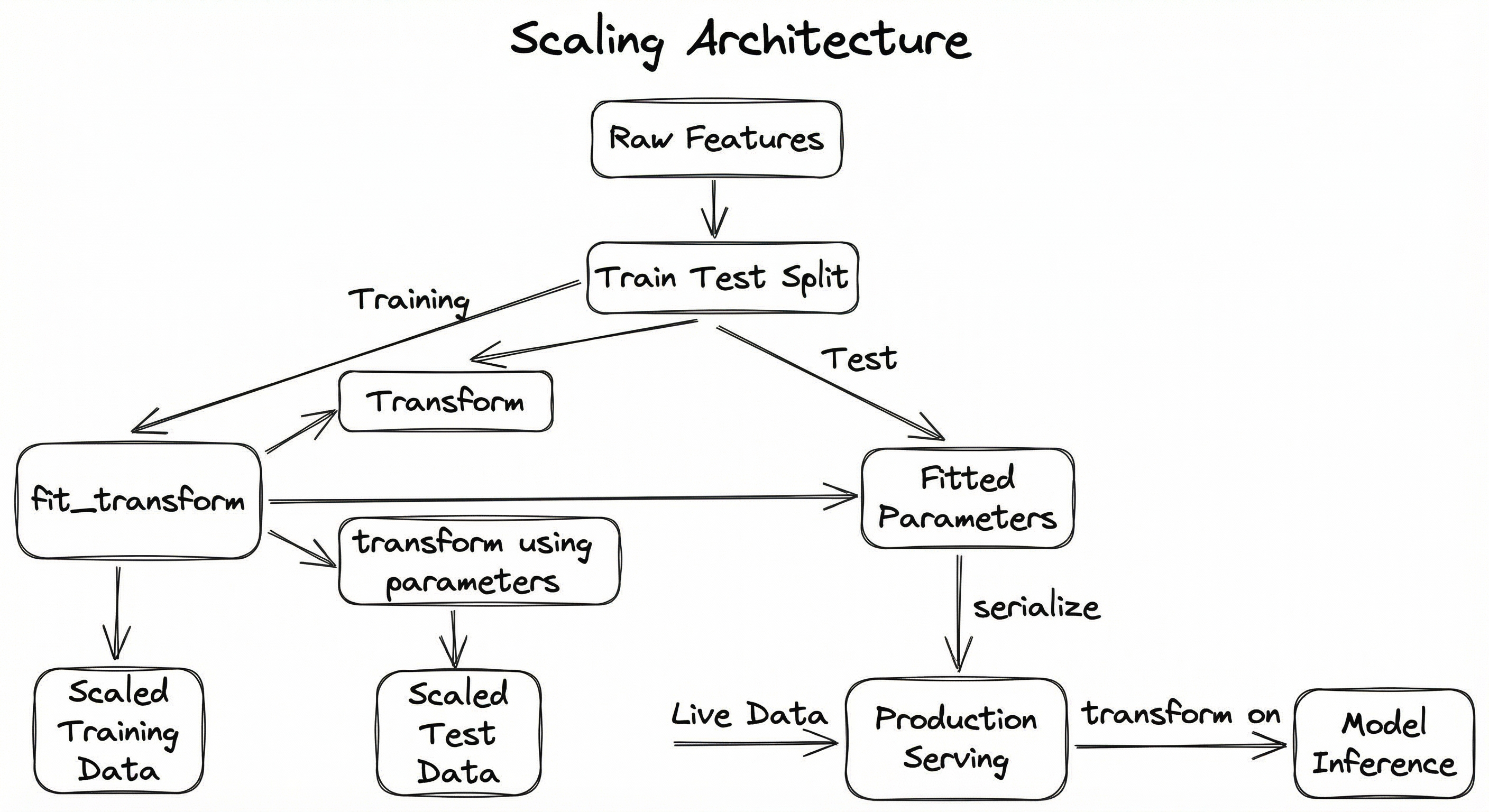
The diagram above illustrates the critical data flow: the scaler is fitted only on training data, and the same fitted parameters are used for test data and production serving. This prevents information from the test set or future data from leaking into the training process.
Key Components
Statistics Computer (Fit Phase)
Computes the scaling parameters from training data: mean/std for StandardScaler, min/max for MinMaxScaler, median/IQR for RobustScaler, quantile breakpoints for QuantileTransformer, or the optimal lambda for PowerTransformer. This runs once per training cycle.
Transformer (Transform Phase)
Applies the stored parameters to transform input features. This runs on every data point -- training, validation, test, and production. Must be deterministic and fast (typically per sample).
Parameter Store
Persists the fitted scaling parameters (means, standard deviations, quantile maps, etc.). In scikit-learn, these are attributes like scaler.mean_ and scaler.scale_. In production, these must be serialized (pickle, ONNX, or custom format) and versioned alongside the model.
Pipeline Orchestrator
Ensures the scaler is applied in the correct order relative to other preprocessing steps (imputation -> scaling -> encoding -> model). scikit-learn's Pipeline and ColumnTransformer serve this role. In production, feature stores like Uber's Michelangelo Palette or Google Vertex AI Feature Store handle this.
Validation Guard
Monitors for distribution drift between training-time statistics and production-time input distributions. Alerts when incoming features fall outside the expected range, indicating either a data pipeline issue or genuine distribution shift that warrants re-fitting the scaler.
Data Flow
Training Path: Raw features arrive -> train/test split is performed -> scaler.fit() computes statistics on training set only -> scaler.transform() applies the transformation to both training and test sets -> scaled data is fed to the model.
Serving Path: Live features arrive at the prediction service -> the serialized scaler (fitted on training data) applies transform() -> scaled features are passed to the model for inference.
Re-training Path: When the model is retrained on new data, the scaler must be re-fit on the new training set. The old scaler parameters are archived (not deleted) to support model rollback. This creates a versioned chain: scaler_v1 + model_v1, scaler_v2 + model_v2, etc.
A directed flow showing raw features split into training and test sets. The training set flows through fit_transform to produce fitted scaler parameters and scaled training data. The test set flows through transform (using the fitted parameters) to produce scaled test data. The fitted parameters are also serialized for production serving, where live data flows through transform before model inference.
How to Implement
Implementation Patterns
There are three main implementation patterns for feature scaling in ML systems:
Pattern 1: scikit-learn Pipeline -- The gold standard for single-machine workflows. Wrapping scalers in a Pipeline ensures correct fit/transform semantics and prevents data leakage during cross-validation. This is what you should use for any model that fits in memory.
Pattern 2: Feature Store Integration -- For production systems at companies like Uber (Michelangelo), Google (Vertex AI Feature Store), or Flipkart, scaling transformations are defined in a feature store or transformation service. The store ensures that the same transformation logic applies during training and serving, preventing training-serving skew.
Pattern 3: In-Database Preprocessing -- Tools like BigQuery ML provide built-in scaling functions (ML.STANDARD_SCALER, ML.MIN_MAX_SCALER) that run inside the data warehouse. This avoids data movement and is cost-effective for large datasets. Google Cloud charges roughly $5 per TB processed (~INR 420/TB), so keeping transformations in BigQuery can save significant egress and compute costs.
Cost Note: For a typical Indian startup processing 10 million records with 50 features, the compute cost of scaling is negligible (under INR 100 / $1.20 on a standard VM). The real cost comes from getting it wrong -- data leakage or training-serving skew can waste weeks of engineering time and degrade model performance silently.
import numpy as np
from sklearn.preprocessing import StandardScaler, MinMaxScaler, RobustScaler

# Sample data: annual income (INR) and age
X_train = np.array([
    [500000, 25],
    [1200000, 35],
    [800000, 28],
    [15000000, 45],   # outlier: very high income
    [600000, 30],
    [900000, 32],
])
X_test = np.array([
    [700000, 27],
    [1100000, 40],
])

# --- StandardScaler ---
std_scaler = StandardScaler()
X_train_std = std_scaler.fit_transform(X_train)
X_test_std = std_scaler.transform(X_test)  # use transform, NOT fit_transform
print("StandardScaler mean:", std_scaler.mean_)
print("StandardScaler std:", std_scaler.scale_)

# --- MinMaxScaler ---
mm_scaler = MinMaxScaler(feature_range=(0, 1))
X_train_mm = mm_scaler.fit_transform(X_train)
X_test_mm = mm_scaler.transform(X_test)
print("MinMax range:", mm_scaler.data_min_, mm_scaler.data_max_)

# --- RobustScaler ---
rob_scaler = RobustScaler()
X_train_rob = rob_scaler.fit_transform(X_train)
X_test_rob = rob_scaler.transform(X_test)
print("RobustScaler median:", rob_scaler.center_)
print("RobustScaler IQR:", rob_scaler.scale_)

# Compare how the outlier (15M income) is handled:
print(f"\nOutlier (row 3, income=15M INR):")
print(f"  StandardScaler: {X_train_std[3, 0]:.2f}")  # large z-score
print(f"  MinMaxScaler:   {X_train_mm[3, 0]:.2f}")    # pushed to 1.0, others compressed
print(f"  RobustScaler:   {X_train_rob[3, 0]:.2f}")   # large but doesn't distort others
This example demonstrates the three core scalers on a realistic dataset with an outlier. Notice how MinMaxScaler compresses all non-outlier incomes into a tiny range near 0 because the outlier (INR 15M) stretches the max. StandardScaler gives the outlier a large z-score but also shifts the mean. RobustScaler handles this best -- the outlier gets a large value, but the median-based centering means the majority of data points are scaled sensibly. The critical pattern to note: fit_transform() on training data, transform() on test data.
from sklearn.pipeline import Pipeline
from sklearn.compose import ColumnTransformer
from sklearn.preprocessing import StandardScaler, OneHotEncoder
from sklearn.linear_model import LogisticRegression
from sklearn.model_selection import cross_val_score
import numpy as np
import pandas as pd

# Simulated Razorpay fraud detection dataset
np.random.seed(42)
df = pd.DataFrame({
    'transaction_amount_inr': np.random.lognormal(10, 2, 1000),
    'time_since_last_txn_sec': np.random.exponential(3600, 1000),
    'merchant_category': np.random.choice(['food', 'electronics', 'travel'], 1000),
    'num_failed_attempts': np.random.poisson(0.5, 1000),
    'is_fraud': np.random.binomial(1, 0.05, 1000),
})

X = df.drop('is_fraud', axis=1)
y = df['is_fraud']

# Define column-specific preprocessing
numeric_features = ['transaction_amount_inr', 'time_since_last_txn_sec', 'num_failed_attempts']
categorical_features = ['merchant_category']

preprocessor = ColumnTransformer(
    transformers=[
        ('num', StandardScaler(), numeric_features),
        ('cat', OneHotEncoder(drop='first', sparse_output=False), categorical_features),
    ]
)

# Pipeline ensures scaler is fit ONLY on training folds
pipeline = Pipeline([
    ('preprocessor', preprocessor),
    ('classifier', LogisticRegression(max_iter=1000, C=0.1)),
])

# Cross-validation automatically handles fit/transform correctly
scores = cross_val_score(pipeline, X, y, cv=5, scoring='roc_auc')
print(f"ROC-AUC: {scores.mean():.3f} +/- {scores.std():.3f}")

# WRONG way (data leakage):
# scaler = StandardScaler()
# X_scaled = scaler.fit_transform(X)  # <-- fits on ALL data including test
# scores = cross_val_score(LogisticRegression(), X_scaled, y, cv=5)
This is the most important code example in this entire guide. The Pipeline ensures that during each cross-validation fold, the StandardScaler is fit only on the training portion and applied to the validation portion. The commented-out "WRONG" approach at the bottom shows the classic data leakage mistake: fitting the scaler on the entire dataset before splitting. This leaks test-set statistics into training and produces over-optimistic evaluation metrics. In a fraud detection system handling crores of INR in transactions, this kind of leakage can mean deploying a model that performs 5-10% worse in production than in evaluation.
import numpy as np
from sklearn.preprocessing import PowerTransformer, QuantileTransformer
import warnings
warnings.filterwarnings('ignore')

# Highly skewed data: e-commerce order values (INR)
np.random.seed(42)
order_values = np.random.lognormal(mean=7, sigma=1.5, size=(1000, 1))
print(f"Original skewness: {float(np.mean((order_values - order_values.mean())**3) / order_values.std()**3):.2f}")
print(f"Original range: [{order_values.min():.0f}, {order_values.max():.0f}]")

# --- PowerTransformer (Yeo-Johnson) ---
pt = PowerTransformer(method='yeo-johnson', standardize=True)
order_pt = pt.fit_transform(order_values)
print(f"\nPowerTransformer (Yeo-Johnson):")
print(f"  Lambda: {pt.lambdas_[0]:.4f}")
print(f"  Skewness after: {float(np.mean((order_pt - order_pt.mean())**3) / order_pt.std()**3):.2f}")

# --- PowerTransformer (Box-Cox, requires positive data) ---
pt_bc = PowerTransformer(method='box-cox', standardize=True)
order_bc = pt_bc.fit_transform(order_values)  # works because all values > 0
print(f"\nPowerTransformer (Box-Cox):")
print(f"  Lambda: {pt_bc.lambdas_[0]:.4f}")
print(f"  Skewness after: {float(np.mean((order_bc - order_bc.mean())**3) / order_bc.std()**3):.2f}")

# --- QuantileTransformer ---
qt = QuantileTransformer(n_quantiles=100, output_distribution='normal', random_state=42)
order_qt = qt.fit_transform(order_values)
print(f"\nQuantileTransformer (to normal):")
print(f"  Skewness after: {float(np.mean((order_qt - order_qt.mean())**3) / order_qt.std()**3):.2f}")
print(f"  Range: [{order_qt.min():.2f}, {order_qt.max():.2f}]")
E-commerce order values are almost always right-skewed (many small orders, few large ones). A StandardScaler would not fix the underlying skewness -- it would just shift and scale it. PowerTransformer applies a parametric transformation (Box-Cox or Yeo-Johnson) that minimizes skewness via maximum likelihood estimation. QuantileTransformer takes a non-parametric approach, mapping values to their quantile rank and then to the target distribution. Both produce near-Gaussian outputs, which is what models like logistic regression and neural networks expect.
import joblib
import json
import numpy as np
from sklearn.preprocessing import StandardScaler
from sklearn.pipeline import Pipeline
from sklearn.linear_model import LogisticRegression

# Train and save
X_train = np.random.randn(1000, 5)
y_train = np.random.binomial(1, 0.3, 1000)

pipeline = Pipeline([
    ('scaler', StandardScaler()),
    ('model', LogisticRegression()),
])
pipeline.fit(X_train, y_train)

# Serialize the entire pipeline (scaler + model together)
joblib.dump(pipeline, 'fraud_model_v2.joblib')

# --- At serving time ---
loaded_pipeline = joblib.load('fraud_model_v2.joblib')

# Single prediction (e.g., from a FastAPI endpoint)
new_transaction = np.array([[50000, 120, 3, 0.8, 1]])  # raw features
prediction = loaded_pipeline.predict_proba(new_transaction)
print(f"Fraud probability: {prediction[0][1]:.4f}")

# Export scaler parameters for non-Python serving (e.g., Go, Java)
scaler = loaded_pipeline.named_steps['scaler']
scaler_params = {
    'mean': scaler.mean_.tolist(),
    'scale': scaler.scale_.tolist(),
    'var': scaler.var_.tolist(),
}
with open('scaler_params_v2.json', 'w') as f:
    json.dump(scaler_params, f, indent=2)
print("Scaler params exported for cross-language serving")
In production, the scaler and model must be serialized together to prevent version mismatches. Using joblib.dump on the entire pipeline ensures that the correct scaler parameters are always paired with the correct model weights. For serving in non-Python environments (common at Indian companies using Go or Java backends), we export the scaler parameters as JSON. The serving application then applies the same mean-subtraction and division before calling the model.
# Feature scaling configuration (YAML)
preprocessing:
  numerical_features:
    - name: transaction_amount_inr
      scaler: robust          # outlier-prone
      params:
        quantile_range: [25, 75]
    - name: user_age
      scaler: standard        # approximately Gaussian
    - name: session_duration_sec
      scaler: power            # heavily skewed
      params:
        method: yeo-johnson
    - name: pixel_values
      scaler: minmax           # need [0, 1] range for neural net
      params:
        feature_range: [0, 1]
  categorical_features:
    - name: merchant_category
      encoder: onehot
      scaler: none             # never scale categorical
  pipeline:
    order: [imputer, scaler, encoder, model]
    prevent_leakage: true
    serialize_format: joblib
    version: v2.1
Common Implementation Mistakes
- ●
Data Leakage via fit_transform on full dataset: Calling
scaler.fit_transform(X)before the train/test split leaks test-set statistics into training. This is the single most common scaling mistake, and it silently inflates evaluation metrics by 2-10%. Always fit on training data only. - ●
Scaling the target variable unintentionally: Applying the scaler to the entire DataFrame including the label column. StandardScaler on a binary classification target (0/1) will produce nonsensical predictions. Use
ColumnTransformerto explicitly select feature columns. - ●
Forgetting to scale at inference time: Training with scaled features but serving with raw features. The model receives inputs in a completely different distribution, producing garbage predictions. This is a training-serving skew bug that can be hard to detect because the model still produces outputs -- they are just wrong.
- ●
Scaling categorical or ordinal features: Applying StandardScaler to one-hot encoded columns or ordinal features like 'low/medium/high' mapped to 1/2/3. These should not be scaled -- they have inherent meaning at their original values. Use
ColumnTransformerto route different feature types to different transformers. - ●
Re-fitting the scaler on each batch during online serving: If you re-fit the scaler on each incoming batch of production data, the scaling parameters drift over time and the model sees a shifting input distribution. The scaler must be fitted once during training and frozen for serving.
- ●
Scaling tree-based model inputs unnecessarily: Applying StandardScaler before XGBoost or Random Forest adds computational overhead and code complexity without any benefit. Tree-based models are invariant to monotonic feature transformations.
When Should You Use This?
Use When
Training any gradient-based model (neural networks, logistic regression, linear regression, SVMs) where convergence speed matters
Using distance-based algorithms (KNN, K-Means, DBSCAN, SVM with RBF kernel) where feature magnitudes directly affect distance calculations
Applying regularization (L1/L2) where you need penalties to treat all features fairly regardless of their natural scale
Working with PCA or SVD where the decomposition is sensitive to feature variance (unscaled features with large variance dominate principal components)
Features have vastly different units (e.g., salary in INR alongside age in years, temperature in Celsius alongside pressure in Pascals)
Building ensemble stacking models where base models include both tree-based and linear models -- scale for the linear models even if trees do not need it
Training deep learning models where input normalization is a standard practice to prevent vanishing/exploding gradients in early layers
Avoid When
Using tree-based models exclusively (Decision Trees, Random Forest, XGBoost, LightGBM, CatBoost) -- they split on thresholds and are invariant to monotonic transformations
Features are already on comparable scales (e.g., all features are percentages between 0 and 100, or all are binary indicators)
Working with sparse data (e.g., TF-IDF matrices) where StandardScaler would destroy sparsity -- use MaxAbsScaler instead if scaling is needed
The model includes built-in normalization (e.g., batch normalization layers in a deep network may make input scaling less critical, though it is still recommended)
Features represent counts or ordinal values where the absolute magnitude carries meaning (e.g., 'number of children' should not be z-scored to -1.3)
You are building a rule-based system or decision rules where human-readable thresholds matter (scaled values like 1.73 standard deviations are harder to interpret than 'income > 10 lakh INR')
Key Tradeoffs
Scaler Comparison Matrix
| Scaler | Outlier Robust | Preserves Shape | Bounded Output | Preserves Sparsity | Gaussianizes |
|---|---|---|---|---|---|
| StandardScaler | No | Yes | No | No | No |
| MinMaxScaler | No | Yes | Yes | No | No |
| RobustScaler | Yes | Yes | No | No | No |
| MaxAbsScaler | No | Yes | Yes | Yes | No |
| PowerTransformer | Moderate | No | No | No | Yes |
| QuantileTransformer | Yes | No | Configurable | No | Yes |
The Outlier Dilemma
The biggest practical tradeoff is outlier sensitivity vs. simplicity. StandardScaler is the default choice because it is simple, fast, and well-understood. But if your dataset has outliers (and most real-world datasets do), the mean and standard deviation will be skewed, and the scaled values for the majority of your data will be suboptimal.
RobustScaler solves this by using median and IQR, but the output is not zero-mean/unit-variance, which some models assume. In practice, the performance difference is often small (1-3% accuracy), but in high-stakes applications like fraud detection at Razorpay or credit scoring at CRED, that 1-3% can translate to crores of INR in losses.
Memory and Compute Tradeoffs
For most scalers, both fit and transform are and the memory footprint is -- trivially small. The exception is QuantileTransformer, which stores quantile values (default ). For a dataset with 10,000 features, that is 10 million stored values -- still manageable but worth noting for memory-constrained edge deployments.
Rule of Thumb: Start with StandardScaler. If you see outlier-driven issues in residual plots or feature importance analysis, switch to RobustScaler. If the data is heavily skewed, apply PowerTransformer first. Only reach for QuantileTransformer when parametric transforms are not enough.
Alternatives & Comparisons
Feature scaling transforms each feature column to a standard range. Sample-wise normalization (sklearn's Normalizer) transforms each row to unit norm. They solve different problems: use feature scaling when features have different units, use row normalization when the magnitude of the entire feature vector is irrelevant (e.g., in text TF-IDF vectors where you care about relative term frequencies, not document length).
Encoding transforms categorical features into numerical representations, while scaling transforms already-numerical features to comparable ranges. They are complementary, not alternatives -- a typical pipeline applies encoding to categorical features AND scaling to numerical features, often via ColumnTransformer. Never apply StandardScaler to one-hot encoded columns.
Feature extraction creates new features (often lower-dimensional) from existing ones, while scaling preserves the original features at adjusted magnitudes. Note that PCA should almost always be preceded by scaling because it is variance-sensitive. If you apply PCA to unscaled data, the first principal component will simply capture the highest-magnitude feature rather than the direction of greatest variance.
Feature selection reduces the number of features; scaling adjusts their values. These are independent operations, but scaling can affect selection: filter methods based on variance or correlation may produce different results on scaled vs. unscaled data. Apply scaling before variance-based feature selection to ensure fair comparison across features.
Pros, Cons & Tradeoffs
Advantages
Dramatically faster convergence for gradient-based models: a well-scaled dataset can converge 10-100x faster than an unscaled one, reducing training time from hours to minutes on the same hardware
Prevents feature dominance: ensures that features with large numerical ranges (e.g., INR salary) do not overshadow informative but small-range features (e.g., number of defaults)
Enables fair regularization: L1/L2 penalties apply uniformly across features, so the model can select or shrink features based on informational value rather than numerical scale
Improves numerical stability: prevents floating-point overflow/underflow in activation functions (sigmoid, softmax) and matrix operations, especially critical for deep learning
Trivially cheap: scaling a million samples with 100 features takes milliseconds on a single CPU core; the ROI is enormous relative to the compute cost
Standardized API: scikit-learn's fit/transform pattern is universally adopted, making scalers plug-and-play across any preprocessing pipeline
Enables meaningful coefficient comparison: in linear models, standardized coefficients directly indicate relative feature importance
Disadvantages
Does not fix skewness: StandardScaler and MinMaxScaler preserve the shape of the distribution -- if data is heavily skewed, you need PowerTransformer or QuantileTransformer first
Outlier sensitivity (StandardScaler and MinMaxScaler): a single outlier can distort the scaling of the entire feature, compressing the majority of values into a narrow range
Data leakage risk: incorrect usage (fitting on full data before splitting) is a pervasive mistake that produces over-optimistic metrics and underperforming production models
Training-serving skew: the scaler parameters must be serialized and versioned with the model; mismatches between training and serving scalers silently degrade predictions
Not universally needed: applying scalers to tree-based models adds unnecessary complexity and can confuse team members who then struggle to interpret raw feature values
Destroys interpretability for domain experts: a doctor understands 'blood pressure = 140 mmHg' but not 'blood pressure = 1.73 standard deviations above the mean'
Sparse data handling: StandardScaler densifies sparse matrices, potentially causing memory issues with high-dimensional sparse data like text features
Failure Modes & Debugging
Data Leakage from Scaling Before Split
Cause
Calling scaler.fit_transform(X) on the entire dataset before performing the train/test split. The scaler learns statistics (mean, std, min, max) that include information from the test set.
Symptoms
Cross-validation and holdout test metrics appear 2-10% better than production performance. The model seems to perform well during development but underperforms in deployment. Difficult to detect without a held-out set that was truly never touched during preprocessing.
Mitigation
Always use scikit-learn's Pipeline with cross_val_score or GridSearchCV. The pipeline ensures fit is called only on training folds. For custom training loops, enforce the pattern: scaler.fit(X_train) then scaler.transform(X_test). Add a unit test that verifies the scaler's mean_ attribute matches the training set statistics, not the full dataset.
Training-Serving Skew
Cause
The scaler used during model training is different from the one applied during serving. This happens when: (a) the scaler is re-fitted on a different dataset in the serving path, (b) the scaler parameters are hardcoded incorrectly, or (c) the scaler version is out of sync with the model version.
Symptoms
Production predictions are systematically biased (shifted up or down). Feature distributions at serving time look correct in isolation, but model outputs are incorrect. A/B tests show the model underperforming its offline evaluation metrics.
Mitigation
Serialize the scaler inside the model pipeline (e.g., joblib.dump(pipeline)) so they cannot be separated. Use a model registry (MLflow, Weights & Biases, or Vertex AI Model Registry) that versions the scaler and model as a single artifact. Add monitoring to compare the distribution of scaled features at training time vs. serving time.
Outlier-Driven Compression (MinMaxScaler)
Cause
A single extreme outlier sets the min or max, compressing all other values into a narrow range. For example, if 99% of transaction amounts are between INR 100 and INR 10,000 but one transaction is INR 10,00,000 (10 lakh), MinMaxScaler compresses the 99% into the range [0, 0.01].
Symptoms
After scaling, the feature histogram shows almost all values clustered near 0 (or 1). The model effectively treats this feature as a constant for most samples, losing its discriminative power. Feature importance drops unexpectedly for features known to be informative.
Mitigation
Use RobustScaler instead of MinMaxScaler when outliers are present. Alternatively, clip outliers before scaling: np.clip(X, np.percentile(X, 1), np.percentile(X, 99)). Or use QuantileTransformer which is inherently robust to outliers. Always plot feature distributions after scaling to visually verify.
Sparse Matrix Densification
Cause
Applying StandardScaler or MinMaxScaler to sparse matrices (e.g., TF-IDF, count vectors). StandardScaler subtracts the mean, turning every zero into a non-zero value, which densifies the matrix.
Symptoms
Memory usage spikes dramatically (e.g., a 1 GB sparse matrix becomes a 50 GB dense matrix). The process crashes with OOM errors. Even if it fits in memory, downstream operations are orders of magnitude slower.
Mitigation
Use MaxAbsScaler for sparse data -- it scales by the maximum absolute value without shifting, preserving all zero entries. Alternatively, use StandardScaler(with_mean=False) to skip the mean subtraction step. For TF-IDF vectors, consider whether scaling is even necessary -- many models work fine with raw TF-IDF values.
New Categories / Out-of-Range Values at Serving Time
Cause
Production data contains feature values outside the range seen during training. For MinMaxScaler, this produces values outside [0, 1]. For QuantileTransformer, values beyond the observed quantile range are clipped.
Symptoms
Predictions for edge cases are unreliable. For MinMaxScaler, out-of-range inputs can produce arbitrarily large (or negative) scaled values, triggering numerical issues in downstream models (e.g., sigmoid saturation in neural networks).
Mitigation
Use MinMaxScaler.clip=True (available in scikit-learn 0.24+) to clip transformed values to the [0, 1] range. Add input validation at serving time to flag features outside the expected range. Retrain periodically if the data distribution is shifting. Consider RobustScaler which is inherently more resilient to range expansion.
QuantileTransformer Distorting Relationships
Cause
QuantileTransformer applies a non-linear transformation that can distort the relationships between features. If two features have a linear relationship, the quantile mapping may make it non-linear.
Symptoms
Linear models perform worse after QuantileTransformer than after StandardScaler, even though the individual feature distributions look more Gaussian. Interaction effects that were simple in the original space become complex.
Mitigation
Only use QuantileTransformer when the model can handle non-linear relationships (e.g., neural networks, gradient boosted trees). For linear models, prefer PowerTransformer which applies a parametric monotonic transformation that preserves more of the original structure. Always compare model performance with and without the non-linear transform.
Placement in an ML System
Pipeline Position
Feature scaling sits in the preprocessing stage of the ML pipeline, specifically:
- Data ingestion (raw data from databases, APIs, files)
- Data cleaning (handle missing values, remove duplicates)
- Imputation (fill remaining missing values) -- MUST happen before scaling
- Feature scaling <-- HERE
- Feature encoding (categorical to numerical) -- often parallel with scaling
- Feature selection (reduce dimensionality)
- Model training
Scaling must happen after imputation because scalers cannot handle NaN values (scikit-learn scalers will raise errors on NaN input). It should happen before feature selection when using variance-based or correlation-based selectors, because unscaled features have incomparable variances.
Interaction with Other Pipeline Components
In a typical Indian fintech pipeline (e.g., Razorpay, PhonePe, or CRED), the feature engineering stage processes dozens of raw signals -- transaction amounts in INR, timestamps, geolocation coordinates, device fingerprints -- into model-ready features. Scaling is one of several transformations applied, alongside log transforms, binning, and encoding. The ColumnTransformer in scikit-learn allows different transformations for different feature groups, which is the standard pattern.
Production Tip: At Uber, the Michelangelo platform embeds transformations (including normalization) directly in the feature pipeline DSL, ensuring that the same transformation applies during training and serving. If you are building a similar system, consider storing scaler parameters in the feature store rather than the model artifact.
Pipeline Stage
Feature Engineering / Preprocessing
Upstream
- data-cleaning
- imputation
- feature-extraction
Downstream
- feature-selection
- model-training
- encoding
Scaling Bottlenecks
Feature scaling itself is rarely a bottleneck -- it is for both fit and transform, which runs in milliseconds even for millions of samples. The bottleneck is operational complexity: ensuring that the same scaler parameters are used across training, evaluation, and serving.
At scale (100M+ samples, 1000+ features), the fit phase for QuantileTransformer can take several minutes because it must sort each feature column to compute quantiles. For real-time serving, the transform phase must complete within single-digit milliseconds, which all scalers achieve easily for a single sample.
The true scaling bottleneck is coordination: when multiple teams use the same features but different scalers, or when the scaler parameters in the feature store drift from those used during training. Companies like Uber and Google address this through centralized feature stores (Michelangelo, Vertex AI Feature Store) that ensure transformation consistency.
Production Case Studies
Uber's Michelangelo platform implements a domain-specific language (DSL) for feature transformations including normalization (subtracting mean and dividing by standard deviation) and bucketization. The DSL ensures that the same transformation logic applies during both model training and real-time serving, preventing training-serving skew. Feature transformations are versioned alongside models in a unified artifact store.
Standardized feature preprocessing across hundreds of ML models reduced training-serving skew incidents and enabled faster model iteration cycles. Michelangelo serves predictions for ETA, pricing, fraud detection, and more -- all relying on consistent feature scaling.
Google's BigQuery ML provides built-in preprocessing functions including ML.STANDARD_SCALER, ML.MIN_MAX_SCALER, ML.MAX_ABS_SCALER, and ML.ROBUST_SCALER that run inside the data warehouse. Scaling transformations are embedded within the trained model, so the same preprocessing applies automatically during both training and prediction. This eliminates the need to export data for preprocessing and prevents training-serving skew.
In-database preprocessing reduces data movement costs and latency. For a dataset of 1 TB (~INR 420 / 50-100 (~INR 4,200-8,400) per training run.
Airbnb's ML team used feature engineering pipelines to predict the value of homes (LTV). Their feature engineering platform Zipline provides pre-computed features at different granularity levels (host, guest, listing, market). For numerical features with skewed distributions (like pricing and review counts), the team applied robust scaling and log transformations to handle outliers common in marketplace data.
The LTV prediction model improved host acquisition targeting, enabling Airbnb to focus marketing spend on high-value properties. Proper feature preprocessing was cited as a critical factor in model accuracy.
Netflix's recommendation system processes hundreds of billions of user interactions. Their RecSysOps framework includes feature quality monitoring that detects when input feature distributions shift -- a critical concern when scaled features are involved. The system monitors for distributional changes that could indicate scaler drift or upstream data pipeline issues, triggering automated alerts and diagnostic workflows.
Proactive monitoring of feature distributions (including scaled feature ranges) reduced the mean time to detect recommendation quality regressions from days to hours.
Tooling & Ecosystem
The reference implementation for feature scaling in Python. Provides StandardScaler, MinMaxScaler, RobustScaler, MaxAbsScaler, PowerTransformer, QuantileTransformer, and Normalizer. All follow the fit/transform API and integrate seamlessly with Pipeline and ColumnTransformer.
A Python library that extends scikit-learn's preprocessing with additional scalers and transformers, including decision-tree-based discretizers and Winsorizers for capping outliers before scaling. Follows the same fit/transform API. Particularly useful for production pipelines that need outlier handling integrated with scaling.
In-database scaling functions (ML.STANDARD_SCALER, ML.MIN_MAX_SCALER, ML.ROBUST_SCALER, ML.MAX_ABS_SCALER) that run inside BigQuery SQL queries. Transformations are embedded in the model, ensuring consistency between training and prediction without data export.
Distributed feature scaling for big data pipelines. Provides StandardScaler, MinMaxScaler, MaxAbsScaler, and Normalizer that run on Spark clusters. Essential for scaling features across datasets that do not fit in memory on a single machine -- common in Indian e-commerce companies processing billions of transactions.
Part of the TFX ecosystem. Defines preprocessing functions that run during both training (on Apache Beam) and serving (as a TensorFlow graph). Supports tft.scale_to_0_1, tft.scale_to_z_score, and custom transformations. Eliminates training-serving skew by baking the transform into the saved model.
A blazing-fast DataFrame library written in Rust with Python bindings. While not a dedicated ML preprocessing tool, its expression-based API makes column-wise scaling operations trivially parallelizable and significantly faster than pandas for large datasets. Increasingly adopted in Indian ML teams for feature engineering at scale.
Research & References
Moreira, Sinaga, et al. (2025)arXiv preprint
Systematic evaluation of 12 scaling techniques across 14 ML algorithms and 16 datasets. Found that ensemble methods (Random Forest, XGBoost, CatBoost, LightGBM) are robust to scaling choice, while logistic regression, SVMs, TabNet, and MLPs show significant performance variation depending on the scaler.
Islam, N. (2024)arXiv preprint
Proposes a novel supervised scaling method that uses decision tree feature importance to scale different features differently via RobustScaler, weighted by their importance. Achieves improved performance on imbalanced datasets.
Ioffe, S. & Szegedy, C. (2015)ICML 2015
Introduced batch normalization -- a learned form of feature scaling applied at every layer of a deep network. Achieved the same accuracy with 14x fewer training steps and demonstrated that internal feature scaling is crucial for deep learning training dynamics.
Yeo, I.-K. & Johnson, R.A. (2000)Biometrika, 87(4), pp. 954-959
Introduced the Yeo-Johnson power transformation that generalizes Box-Cox to handle both positive and negative values. This is the default method in scikit-learn's PowerTransformer and is widely used for Gaussianizing skewed features.
Raju, V.N.G. et al. (2019)International Conference on Intelligent Computing and Communication
Empirically demonstrated that feature scaling reduces the number of iterations required for gradient descent convergence by 2-10x, with StandardScaler and MinMaxScaler showing the most consistent improvements across different learning rates.
Interview & Evaluation Perspective
Common Interview Questions
- ●
When would you use StandardScaler vs. MinMaxScaler vs. RobustScaler?
- ●
Why do tree-based models not require feature scaling?
- ●
How do you prevent data leakage when scaling features in a cross-validation setup?
- ●
A colleague scaled the features before the train/test split. What is the impact?
- ●
How would you handle feature scaling in a production serving pipeline to avoid training-serving skew?
- ●
When would you use PowerTransformer instead of StandardScaler?
- ●
How does feature scaling affect L1 and L2 regularization?
- ●
Your model performs well in offline evaluation but poorly in production. Feature scaling could be the cause -- how would you diagnose this?
Key Points to Mention
- ●
StandardScaler is the default choice for approximately Gaussian data; MinMaxScaler for bounded ranges; RobustScaler for outlier-heavy data -- always justify the choice based on data characteristics, not habit
- ●
Data leakage from scaling is the #1 preprocessing mistake: fit on training data ONLY, then transform both train and test. Use sklearn Pipeline to enforce this automatically
- ●
Tree-based models (RF, XGBoost, LightGBM) do NOT need scaling because splits depend on value ordering, not magnitude. This saves computation and preserves interpretability
- ●
In production, the scaler must be serialized WITH the model (same artifact) to prevent training-serving skew. Version them together in a model registry
- ●
Regularization (L1/L2) is directly affected by feature scale: without scaling, large-magnitude features are effectively unregularized while small-magnitude features are over-penalized
- ●
QuantileTransformer is powerful but non-linear -- it can distort inter-feature relationships. Use it with non-linear models (neural nets, GBDTs), not with linear models
Pitfalls to Avoid
- ●
Saying 'always scale your features' without acknowledging the tree-based model exception -- this shows a lack of understanding of why scaling works
- ●
Confusing feature scaling (column-wise) with sample normalization (row-wise, e.g., L2 normalization) -- they solve different problems
- ●
Forgetting to mention data leakage -- this is the most impactful failure mode and interviewers specifically look for awareness of it
- ●
Claiming that MinMaxScaler is always better than StandardScaler (or vice versa) without discussing data characteristics and outliers
- ●
Not knowing that MaxAbsScaler preserves sparsity while StandardScaler does not -- important for NLP and high-dimensional sparse data
Senior-Level Expectation
A senior ML engineer should discuss the full production lifecycle of feature scaling: choosing the right scaler based on data EDA (distribution shape, outlier analysis), preventing data leakage via Pipeline, serializing scaler parameters alongside the model, monitoring for distribution drift at serving time, and re-fitting strategies when data distributions shift. They should also discuss training-serving skew mitigation patterns (embedding transformations in the model artifact, using feature stores), cost implications of different approaches (in-database vs. external preprocessing), and when scaling is unnecessary (tree-based models, batch-normalized deep networks). The ability to reason about edge cases -- sparse data, out-of-range values at serving time, the impact on regularization fairness -- separates senior engineers from mid-level ones. At companies like Flipkart or Swiggy handling millions of daily transactions, the operational aspects (monitoring scaled feature distributions, automated retraining triggers) matter as much as the statistical correctness.
Summary
Feature scaling is a foundational preprocessing step that transforms numerical features to comparable magnitudes, enabling gradient-based optimization, distance-based algorithms, and regularization to work correctly. The six primary scalers -- StandardScaler (z-score), MinMaxScaler (bounded range), RobustScaler (median/IQR for outliers), MaxAbsScaler (preserves sparsity), PowerTransformer (Gaussianization), and QuantileTransformer (non-parametric distribution mapping) -- each address different data characteristics. The choice depends on your data distribution, outlier prevalence, and model type.
The most critical operational concern is data leakage prevention: the scaler must be fitted on training data only and the same fitted parameters applied to test and production data. scikit-learn's Pipeline enforces this automatically. In production, the scaler must be serialized alongside the model to prevent training-serving skew, and feature distributions should be monitored for drift.
Equally important is knowing when NOT to scale: tree-based models (Random Forest, XGBoost, LightGBM, CatBoost) are invariant to monotonic feature transformations and gain no benefit from scaling. Applying scalers unnecessarily adds complexity without value. The decision framework is straightforward: scale for gradient-based and distance-based models, skip for tree-based models, and use robust or power transformations when outliers or skewness are present. As a preprocessing step, scaling is computationally trivial -- the real investment is in getting the pipeline right.